Power spectrum normalization from the local abundance of rich clusters of galaxies

Abstract

The number density of rich galaxy clusters still provides the most robust way of normalizing the power spectrum of dark matter perturbations on scales relevant to large-scale structure. We revisit this constraint in light of several recent developments: (1) the availability of well-defined samples of local clusters with relatively accurate X-ray temperatures; (2) new theoretical mass functions for dark matter haloes which provide a good fit to large numerical simulations; (3) more accurate mass-temperature relations from larger catalogues of hydrodynamical simulations; (4) the requirement to consider closed as well as open and flat cosmologies to obtain full multi-parameter likelihood constraints for CMB and SNe studies. We present a new sample of clusters drawn from the literature and use this sample to obtain improved results on $\sigma_{8}$, the normalization of the matter power spectrum on scales of $8\,h^{-1}\,$Mpc, as a function of the matter density and cosmological constant in a Universe with general curvature. We discuss our differences with previous work, and the remaining major sources of uncertainty. Final results on the normalization, approximately independent of power spectrum shape, can be expressed as constraints on $\sigma$ at an appropriate cluster normalization scale $R_{\rm Cl}$. We provide fitting formulas for $R_{\rm Cl}$ and $\sigma(R_{\rm Cl})$ for general cosmologies, as well as for $\sigma_{8}$ as a function of cosmology and shape parameter $\Gamma$. For flat models we find approximately $\sigma_{8}\simeq(0.495^{+0.034}_{-0.037})\,\Omega_{\rm M}^{-0.60}$ for $\Gamma=0.23$, where the error bar is dominated by uncertainty in the mass-temperature relation.

1 Introduction

In theories of hierarchical structure formation the class of objects most recently formed holds a special significance. Observationally this class of objects is clusters of galaxies – the largest virialized structures in the present day universe. The local abundance of rich clusters of galaxies provides a strong constraint on the fluctuations in the matter density on scales of order 10 Mpc [Evrard 1989, Frenk et al. 1990, Bond & Myers 1991, Henry & Arnaud 1991, Kaiser 1991, Lilje 1992, Oukbir & Blanchard 1992, Bahcall & Cen 1993, Hanami 1993, White, Efstathiou & Frenk 1993]. Consistency with this constraint is one of the most important tests a model can pass, since the constraint is directly on the linear theory power spectrum, at a scale where there is an abundance of data. By fixing the normalization at wavelengths much smaller than those probed by COBE one obtains an accurate local normalization on scales relevant to much of structure formation, a long lever arm for constraining the shape of the power spectrum, and a normalization to matter fluctuations which is independent of galaxy bias.

There have been several recent and detailed studies of the cluster abundance, including Bond & Myers [Bond & Myers 1996], Eke, Cole & Frenk [Eke et al. 1996], Viana & Liddle [Viana & Liddle 1996, Viana & Liddle 1999], Colafrancesco, Mazzotta & Vittorio [Colafrancesco et al. 1997], Kitayama & Suto [Kitayama & Suto 1997], Eke et al. [Eke et al. 1998], Pen [Pen 1998], Wang & Steinhardt [Wang & Steinhardt 1998], Donahue & Voit [Donahue & Voit1999] and Henry [Henry 2000]. However, even more recently, there have been several developments in terms of both theory and observation which suggest it would be useful to revisit this constraint. Firstly the addition of ASCA temperatures [Tanaka, Inoue & Holt 1994] means that there is now a well defined local temperature function for clusters, with relatively small errors in temperature. Secondly a number of large N-body simulations have accurately determined the mass function of virialized haloes (e.g. Governato et al. 1999), finding non-negligible deviations from the old Press-Schechter (1974; hereafter PS) theory. For example the extremely large N-body simulations of the Virgo consortium have highlighted systematic departures from the PS predicted mass functions [Jenkins et al. 2001], which alter the constraints on the power spectrum normalization coming from the cluster abundance. Thirdly, more ambitious hydrodynamical simulations of cluster formation (e.g. Frenk et al. 1999, and references therein) have resulted in improvements in the relationship between mass and temperature and a better estimate of its scatter. Finally, the increased sophistication of multi-parameter cosmological studies (in particular driven by recent CMB anisotropy measurements) requires that cosmological models with general curvature be considered (see e.g. White & Scott 1996).

With these refinements our results are an improvement over other studies of the past few years. We point out explicitly where we differ from other work, and also where we think things could be further improved in the future. The outline of the paper is as follows: we review some of the appropriate theory in §2; our local sample of clusters is presented in §3; we describe our statistical method in §4; and we present our results and conclusions in §5 and §6.

2 Theory

The abundance of rich clusters is tied to the normalization of the power spectrum (extrapolated to the present using linear theory) through the Press-Schechter (1974) theory and its extensions (see Sheth, Mo & Tormen 2000 and references therein). The theory has always had a somewhat weak analytic justification, its widespread adoption arising from the dual facts that it is easy to use and provides a remarkably good fit to more computationally expensive simulations.

Although galaxy velocity dispersion and gravitational lensing mass estimates exist for many clusters [Carlberg et al. 1996, Smail et al. 1997, Girardi et al. 1998a, Allen 1998, Wu et al. 1998, Girardi et al. 2000], the direct estimation of mass through determination of the X-ray temperature is far more reliable – although the situation is certainly improving, allowing for estimates of the mass function [Girardi et al. 1998b, Borgani et al. 1999]. In the X-ray band there is considerably more high quality data on luminosity than on temperature, but there is enormous uncertainty in deriving mass $M$ from luminosity $L_{\rm X}$. Hence our point of comparison between theory and observation will be the temperature function of rich clusters, i.e. the number density of clusters within a temperature range $dT$ about $T$. This needs to be observationally determined over some range of $T$ sufficiently high that gravitational physics dominates. Observational and theoretical considerations place this limit at $T_{\rm X}\,{\mathrel{\raise 1.50696pt\hbox{$\scriptstyle>$}\kern-6.00006pt\lower 1.72218pt\hbox{{$\scriptstyle\sim$}}}}\,3.5\,$keV (e.g. Finoguenov et al. 2000; Nevalainen, Markevitch & Forman  2000). Ideally we could compare the data with a temperature function estimated directly from a series of large cosmological hydrodynamic simulations (see e.g. Pen 1998), which included all of the physics relevant to determining the emission weighted inter-galactic medium (IGM) temperature of clusters. This however is currently computationally infeasible. Instead we shall make use of the fact that rich clusters are large virialized structures dominated by gravity, and thus we can factorize the problem and proceed in two steps.

First we shall use the abundance of dark matter haloes of a given mass drawn from extremely large N-body simulations. Any dark matter halo large enough to host a cluster is unambiguously seen in such simulations. Next we shall use a mass-temperature relation, calibrated from hydrodynamical simulations, to convert from the (unobservable) virial mass to the IGM temperature, effectively using the larger volume of the N-body simulations to improve the statistics of the hydro simulations. Unfortunately the mass functions determined from the N-body simulations are somewhat dependent on the method used to define haloes and their masses, and the precise definition of mass used there is not exactly what is used in the hydrodynamic simulations which calibrate the $M{-}T$ relation; the difference is expected to be small however [Jenkins et al. 2001]. We discuss further details of the $M{-}T$ relation in §§2.4 and 2.5.

2.1 The mass variance

Our constraint will be on the variance of the density field, smoothed on some (comoving) scale $R$ corresponding to a mass $M=(4\pi/3)\bar{\rho}R^{3}$ where $\bar{\rho}$ is the background density. In terms of the power spectrum

$$\sigma^{2}(R,z)=\int_{0}^{\infty}{dk\over k}\ \Delta^{2}(k,z)W^{2}(kR)\,,$$ (1)

where $\Delta^{2}=k^{3}P(k,z)/(2\pi^{2})$, $P(k)\equiv|\delta_{k}|^{2}$ is the matter power spectrum and $W(kR)$ is the window function corresponding to the smoothing of the density field (see e.g. Peebles 1993). Our mass functions are fitted assuming a spherical top-hat smoothing, so

$$W(kR)=\left[{3j_{1}(kR)\over kR}\right]\,,$$ (2)

where $j_{1}(x)$ is the spherical Bessel function of order 1. We are interested in both the normalization of the power spectrum, for which we shall use $\sigma_{8}\equiv\sigma(8\,h^{-1}\,{\rm Mpc})$, and its shape. We use the Cold Dark Matter family of power spectra and parameterize the shape by $\Gamma$ in the fitting formula of Bardeen et al. (1986). While the form of Eisenstein & Hu (1999) provides a slightly better fit to the shape, we will mostly quote the results in a $\Gamma$ independent way, rendering this distinction unimportant.

We write $\sigma(R,z)=\sigma(R,0)\,g(z)/g(0)$ where the growth factor $g(z)$ can be computed numerically [Heath 1977, Carroll, Press & Turner 1992, Cohn 1999, Hamilton 2001]:

$$g(z)={5\over 2}{\Omega_{\rm M}\over a}{{da}\over{d{\tau}}}\int_{0}^{a}da^{\prime}\left({da^{\prime}}\over{d{\tau}}\right)^{-3},$$ (3)

where the scale factor $a=(1+z)^{-1}$, and the dimensionless time $\tau\equiv H_{0}t$. The Friedmann equation gives

$$\left({\dot{a}\over a}\right)^{2}=H_{0}^{2}\left({\Omega_{\rm M}\over a^{3}}+\Omega_{\Lambda}+{\Omega_{\rm K}\over a^{2}}\right)\,,$$ (4)

where $H_{0}\equiv({\dot{a}}/a)_{t_{0}}$ is the Hubble constant. The usual symbols $\Omega_{\rm M}$, $\Omega_{\Lambda}\equiv\Lambda/3H_{0}^{2}$ and $\Omega_{\rm K}\equiv 1-\Omega_{\rm M}-\Omega_{\Lambda}$ are the density parameters ($\rho/\rho_{\rm crit}$, with $\rho_{\rm crit}=3H_{0}^{2}/8\pi G$) in matter, cosmological constant and curvature, respectively. Photons and other relativistic species can be safely ignored.

2.2 Press-Schechter and modifications

Figure 1: A comparison of the Press-Schechter form for the multiplicity function, used in all previous work, with the Sheth & Tormen (1999) model, which better fits the Virgo simulation results (see text). Note that Press-Schechter systematically underestimates the abundance of the most massive cluster haloes, $\nu\sim 10$, and can either overestimate or underestimate the abundance of more typical clusters with $\nu\sim$ few.

Within the PS theory and its extensions the (comoving) number density of objects of (virial) mass $M$ is a function only of $\sigma(M)$. Using the scaled variable

$$\nu\equiv\left({\delta_{\rm c}\over\sigma(M)}\right)^{2}\,,$$ (5)

with $\delta_{\rm c}\equiv 1.686$, we write the mass function in terms of the ‘multiplicity function’ $f(\nu)$ as

$$\nu f(\nu)={M^{2}\over\bar{\rho}}{dn\over dM}{d\ln M\over d\ln\nu}\,.$$ (6)

In the spirit of using PS as a fitting function to N-body simulations we do not imbue $\delta_{\rm c}$ with a cosmology dependence (see next section) but rather keep it constant. The Press-Schechter model for $f(\nu)$ is

$$\nu f(\nu)=\sqrt{\nu\over 2\pi}e^{-\nu/2},$$ (7)

and this formula has been extensively used to make predictions of cluster abundances in different cosmologies. Recently Sheth & Tormen (1999) have proposed a correction to the Press-Schechter formula, motivated by a model of non-spherical collapse, that better fits large N-body simulations:

$$\nu f(\nu)\propto(1+{\widetilde{\nu}}^{-p})\,{\widetilde{\nu}}^{\,1/2}e^{-{\tilde{\nu}}/2}\,,$$ (8)

where $p=0.3$ and ${\widetilde{\nu}}=0.707\nu$. The normalization is fixed by the requirement that all of the mass be in haloes, i.e.

$$\int f(\nu)d\nu=1\,;$$ (9)

for the above choice of parameters the normalization factor is 0.2162. Jenkins et al. [Jenkins et al. 2001] have shown that Eq. (8) is in very good agreement with the simulations of the Virgo Consortium, except for very rare objects which shall not be of interest in this work. We compare the multiplicity functions in Fig. 1. Note that Press-Schechter systematically overestimates the abundance of objects of cluster mass having ${\rm 1}\,{\mathrel{\raise 1.50696pt\hbox{$\scriptstyle>$}\kern-6.00006pt\lower 1.72218pt\hbox{{$\scriptstyle\sim$}}}}\,\nu\,{\mathrel{\raise 1.50696pt\hbox{$\scriptstyle>$}\kern-6.00006pt\lower 1.72218pt\hbox{{$\scriptstyle\sim$}}}}\,{\rm 6}$ ($\sigma(R)\mathrel{\raise 1.50696pt\hbox{$\scriptstyle<$}\kern-6.00006pt\lower 1.72218pt\hbox{{$\scriptstyle\sim$}}}0.7$) and underestimates the abundance of objects corresponding to a higher $\sigma(R)$.

2.3 Spherical top-hats

The spherical top-hat ansatz [Peebles 1993, Liddle & Lyth 2000, Peacock 1999] models the formation of an object by the evolution of a spherical overdense region embedded in a homogeneous ‘background’ of mean density $\bar{\rho}$. This region begins by expanding at the same rate as the background, but since it is positively curved the expansion slows, comes to a halt and the region collapses. Mathematically the evolution proceeds to a point of zero radius, however physically we assume that virialization occurs at twice the turn-around time, resulting in a sphere of half the turn-around radius. The overdensity (relative to the background) at turn-around is $9\pi^{2}/16$ for an Einstein-de Sitter model. At virialization the background has become less dense and the sphere’s density grown by a further factor of 8 – we then denote the overdensity relative to the critical density by $\Delta_{\rm c}$. This parameter has the value $18\pi^{2}$ in an Einstein-de Sitter model, and will in general be a function of $\Omega_{\rm M}$ and $\Omega_{\Lambda}$. The extrapolation from linear theory of this overdensity is normally denoted $\delta_{\rm c}$. It is $(3/20)(12\pi)^{2/3}\simeq 1.686$ for Einstein-de Sitter and varies by a few percent in other cosmologies. This density is used as a threshold in PS theory and its extensions. We shall neglect the small cosmology dependence and simply take $\delta_{\rm c}$ fixed throughout.

The value of the density contrast at collapse, $\Delta_{\rm c}$, on the other hand, should be calculated for each model, since it will be important for the $M{-}T$ relation. We computed $\Delta_{\rm c}$ by numerically integrating the equations of motion for the spherical top-hat collapse, including the correction to the virial theorem from the $\Lambda r^{2}$ potential (Lahav et al. 1991; §4.2). Our results can be fit to 2 per cent over the range $0.2\leq\Omega_{\rm M}\leq 1.1$ and $0\leq\Omega_{\Lambda}\leq 1$ by

$$\Delta_{\rm c}=\Omega_{\rm M}\sum_{i,j=0}^{4}c_{ij}\ x^{i}y^{j}\,,$$ (10)

where $x\,{\equiv}\,\Omega_{\rm M}-0.2$, $y\,{\equiv}\,\Omega_{\Lambda}$ and the coefficients $c_{ij}$ are reported in Table 1. As an example we plot $\Delta_{\rm c}$ vs $\Omega_{\rm M}$ for flat models, where the dashed line shows our fit and the solid line is the exact relation. We also checked this fit with the one provided by Eke, Navarro & Frenk. (1998b) and found an agreement at the 1 per cent level. Note that some authors use a different convention in which $\Delta_{\rm c}$ is specified relative to the background matter density – our $\Delta_{\rm c}$ is $\Omega_{\rm M}$ times theirs.

Table 1: Coefficients $c_{ij}$ of the fitting formula, Eq. (10), for the collapse overdensity $\Delta_{\rm c}$.

	$j$
$i$	0	1	2	3	4
0	$546.67$	$-137.82$	$94.0830$	$-204.680$	$111.51$
1	$-1745.6$	$627.22$	$-1175.2$	$2445.7$	$-1341.7$
2	$3928.8$	$-1519.3$	$4015.80$	$-8415.3$	$4642.1$
3	$-4384.8$	$1748.7$	$-5362.1$	$11257.$	$-6218.2$
4	$1842.3$	$-765.53$	$2507.7$	$-5210.7$	$2867.5$

Figure 2: Showing our fit to the overdensity at virialization, $\Delta_{\rm c}$ vs $\Omega_{\rm M}$ for flat models, where the dashed curve is our fitting function and the solid curve is the exact result.

2.4 Halo mass definitions

Before we turn to the mass-temperature relation we note a few important details about determining the mass of a dark-matter halo. Unfortunately there is no unique algorithmic definition of a dark matter halo, even within a 3D simulation itself. Some particular group finders are in common use, but no single group finder is always used. For large objects such as clusters all group finders should be able to find all of the clusters, so this is not of immediate concern, although the degree of substructure will be highly variable between group finders.

More disconcertingly there are a wide number of definitions of halo mass in the literature, and they can differ by a large amount. Even for the mass-temperature relations calibrated by hydro simulations different authors use different definitions of ‘mass’, with the differences dependent on the cosmological parameters. In this sub-section we briefly review the relevant mass definitions and discuss which is the most appropriate for the mass function of Eq. (8).

Although other halo finders are in common use, we shall deal exclusively with haloes found using the Friends-of-Friends (Davis et al. 1985) algorithm, hereafter called FOF. The FOF algorithm has one free parameter, $b$, the linking length in units of the mean inter-particle spacing. Commonly used values of $b$ are 0.1, 0.15 and 0.2. The mass of the halo is simply the sum of the masses of the particles identified as part of the halo. An alternative (and more easily interpreted) procedure is to use FOF to find candidate haloes, identify a halo centre (e.g. the centre of mass of the halo or, more robustly, the position of the most bound particle) and then to calculate the mass from the spherically averaged density profile about that centre. This is the technique typically used to define the mass in hydrodynamic simulations which calibrate the $M\,{-}\,T$ relation.

In this spirit we define $M_{\Delta}$ as the mass contained within a radius $r_{\Delta}$, inside of which the mean interior density is $\Delta$ times the critical density:

$$\int_{0}^{r_{\Delta}}r^{2}dr\ \rho(r)={\Delta\over 3}\rho_{\rm crit}r_{\Delta}^{3}\,.$$ (11)

The ‘virial mass’ from the spherical top-hat collapse model would then be simply $M_{\Delta_{\rm c}}$. Other masses in common use are $M_{500}$ and $M_{200}$ where the latter is approximately the virial mass if $\Omega_{\rm M}=1$.

For large mass haloes many of these definitions are related on average simply by a factor. We can estimate this factor by assuming that haloes have a universal profile, for example the NFW form (Navarro, Frenk & White 1996):

$$\rho(r)\propto x^{-1}\left(1+x\right)^{-2},$$ (12)

where $x=r/r_{\rm s}$ and $r_{\rm s}$ is a scale radius usually specified in terms of the concentration parameter $c\equiv r_{200}/r_{\rm s}$. Navarro et al. (1996) refer to $r_{200}$ and $M_{200}$ throughout as the ‘virial radius’ and ‘virial mass’ respectively. Again, N-body simulations have shown that the concentration parameter is a weak function of virial mass, having the value $c\sim 5$ for masses characteristic of clusters. We can use this profile to relate the various mass definitions, as shown in Fig. 3.

Unfortunately, while this model works well for converting between spherically averaged mass definitions based on $M_{\Delta}$, there is a large scatter for masses based on group membership, such as $M_{{\rm fof}0.2}$. This is because with $b=0.2$, FOF can link together neighbouring haloes in supercluster-like structures, increasing the mass assigned to the structure compared to the $M_{\Delta}$ estimators. Thus the ‘FOF’ lines in Fig. 3 must be taken as highly uncertain. Comparing the mass function from a high-resolution N-body simulation (of the Ostriker & Steinhardt 1995 concordance model) with the universal form of Jenkins et al. [Jenkins et al. 2001] we find the best match is obtained if we interpret their mass as $M_{\Delta_{\rm c}}$. We shall assume below that this remains true independent of cosmology. But we note that this ambiguity in the definition of mass remains a significant source of uncertainty.

Figure 3: Relations between various definitions of the mass of a halo as a function of $\Omega_{\rm M}$ assuming the halo density profile follows the NFW form with concentration parameter $c=5$. The FOF based masses are only crude approximations in this model (see text).

2.5 The M–T relation

The mass function of rich clusters is itself not observable. However the local temperature function is reasonably well known (see §3). To predict the latter from the former we need a relation between emission weighted IGM temperature and cluster virial mass. Our results are quite sensitive to the choice of $M{-}T$ relation, and currently the uncertainty in this relation is the largest theoretical source of error in determining $\sigma_{8}$ (see also Voit 2000).

Recent observational determinations of the mass-temperature relation [Horner, Mushotsky & Scharf 1999, Nevalainen, Markevitch & Forman 2000] disagree at the several tens of percent level (in mass at fixed temperature) when using different estimators of the cluster mass. The virial mass of a cluster is a notoriously difficult quantity to obtain observationally with high accuracy – while different estimators clearly correlate well, they disagree at the level of accuracy required here. Such observations do however provide general support for the functional form and scalings predicted by the spherical collapse model (see below) for clusters of sufficiently large mass. Similar scalings are seen in hydrodynamic simulations of galaxy clusters in a cosmological context. In the simulations the total mass of a cluster is easy to obtain (though convention dependent, §2.4) and in what follows we shall use a $M{-}T$ relation derived from simulations. While these hydrodynamic simulations show good agreement for the total mass and X-ray temperature properties of clusters (Frenk et al. 1999) there are several uncertainties which enter when comparing the simulations to observations and which are important to note.

As with all simulation derived results there are issues related to numerical convergence. With the latest round of high resolution simulations the situation in this respect has improved dramatically. However, the spectrally measured cluster temperatures may not coincide with the mass or emission weighted temperature estimated from the simulations, due to the influence of soft line emission [Mathiesen & Evrard 2001]. Secondly, most simulations are done with purely adiabatic hydrodynamics, which ceases to be a good model for the lower mass/temperature clusters. It is also possible that energy injection (possibly from SNe, AGN or galaxies) has altered the $M{-}T$ relation, again an effect thought to operate preferentially on lower mass/temperature clusters. Thirdly the simulations usually predict the emission weighted temperature, which only converges if data are used out to a radius ${\sim}\,r_{500}$. Observers often probe different ranges of radius in determining the cluster temperature and perform more sophisticated modelling, which can lead to discrepancies between the measured and simulated temperatures. Finally, there still remain significant (for our purposes) calibration uncertainties for the detectors.

With these caveats in mind, the results from the simulations can be quoted in terms of corrections to the spherical collapse model which relates the mass to the (virial) temperature of the hot IGM. For an object virialized at a redshift $z$ we have

$$\left({M(T,z)\over 10^{15}\,h^{-1}\,{\rm M}_{\odot}}\right) = \left({T\over\beta}\right)^{3/2}\left(\Delta_{\rm c}E^{2}\right)^{-1/2}\times$$ (13)

$$\left[1-2{\Omega_{\Lambda}(z)\over\Delta_{\rm c}}\right]^{-3/2}\ ,$$

where $T$ is in keV, $\Delta_{\rm c}$ is the mean overdensity inside the virial radius in units of the critical density and, from Eq. (4), $E^{2}=\Omega_{\rm M}(1+z)^{3}+\Omega_{\Lambda}+\Omega_{\rm k}(1+z)^{2}$. Note that $\Delta_{\rm c}$ is a redshift dependent variable, and should be evaluated using the appropriate $\Omega_{\Lambda}(z)$ and $\Omega_{\rm M}(z)$. The term in square brackets is a correction to the virial relation arising from the additional $r^{2}$ potential in the presence of $\Lambda$ [Lahav et al. 1991, Viana & Liddle 1996, Wang & Steinhardt 1998]. It provides only a small correction and, though we include it, it can be neglected at the present level of accuracy.

Table 2: The mass-temperature relation determined from hydrodynamical simulations. The quoted value of $\beta$ is that relevant for use in Eq. (13). From top to bottom the references are: EMN [Evrard et al. 1996]; ENF [Eke et al. 1998]; BN [Bryan & Norman 1998]; YJS [Yoshikawa, Jing & Suto 2000]; TC [Tittley & Couchman 2000] and Tetal [Thomas et al. 2000]. We have quoted emission weighted temperatures where available, while the last two values (marked with an asterisk) are core temperatures.

Name	$\Omega_{\rm M}$	$\Omega_{\Lambda}$	$\Omega_{\rm B}$	h	$\beta$
EMN	1.0	0.0	0.10	0.50	1.21
EMN	0.2	—	0.10	0.50	1.42
ENF	0.3	0.7	0.04	0.70	1.33
BN	1.0	0.0	0.06	0.50	1.10
BN	1.0	0.0	0.10	0.65	1.04
BN	1.0	0.0	0.08	0.50	1.04
BN	0.4	0.0	0.06	0.65	1.08
YJS	0.3	0.7	0.03	0.70	1.48
TC∗	1.0	0.0	0.10	0.65	1.61
Tetal∗	1.0	0.0	0.06	—	1.23

Ideally the normalization and scatter of the $M{-}T$ relation would be determined by simulations, so that theoretical models can be compared with the data rather more directly (e.g. Pen 1998). However Eq. (13) is a remarkably good fit to the simulations, which are sufficiently computationally demanding that they cannot explore parameter space efficiently. Thus we rely on a hybrid approach where the coefficients are determined from simulations, while the scalings are taken from simple theoretical models [Mathiesen 2000]. Specifically we use the hydrodynamic simulations to determine $\beta$, together with Eq. (13) for the mass and redshift dependence. In practice we used the $M{-}T$ relation at an observed $z=0.053$, corresponding to the median redshift of our cluster sample (see §3). We then shift the resulting $\sigma(z=0.053)$ value to $z=0$ using the growth rate, Eq. (3), which is a significant 5 per cent correction.

The simulations normalize $\beta$ assuming that the virialization redshift is the redshift of observation. In principle one could attempt to correct for the virialization redshift dependence, however we have chosen not to do this, and here we differ from Viana & Liddle [Viana & Liddle 1999] and Wang & Steinhardt (1998), for example. The simulations, which clearly include the full effects of variations in the virialization redshift, give an $M{-}T$ relation well fit by Eq. (13) if $z$ is interpreted as the redshift of observation. We believe that the effect of differing virialization redshifts is included in the simulations as part of the scatter about the mean relation (see below), and so to add an additional effect by hand would be incorrect. Comparison of the scatter in the $M{-}T$ relation found by Bryan & Norman (1998) in a full cosmological simulation with that of Evrard, Metzler & Navarro (1996), who use constrained realizations (and thus constrained formation times), suggests that in fact the effect of scatter in the virialization redshift is a very small source of the total scatter in the relation. Most of the scatter is due to the different merging histories (see also Cavaliere, Menci & Tozzi 1999). While further simulations will be needed to address this issue properly, recent work (Mathiesen 2000) suggests that minor merger events have a more important influence on the evolution of the temperatures than major mergers (and hence formation time).

A summary of recent numerical experiments which constrain $\beta$ is given in Henry [Henry 2000]. We have taken Henry’s list, added some recent work and corrected one of the relations to use $M_{\rm vir}$. Our results are shown in Table 2. The $M{-}T$ relation of Evrard et al. [Evrard et al. 1996] defines mass as $M_{200}$, so that in the context of the spherical top-hat model there is predicted to be an $\Omega_{\rm M}$ dependence to the prefactor of the scaling relation. Correcting for this scaling brings the $\beta$s obtained in these simulations into better agreement, but they still disagree slightly, suggesting that the scaling is only approximately observed. We postulate that this is because $\Omega_{\rm B}/\Omega_{\rm M}$ changes drastically between the simulations. The $M$s of Eke et al. [Eke et al. 1998], Bryan & Norman [Bryan & Norman 1998], and Yoshikawa et al. [Yoshikawa, Jing & Suto 2000], on the other hand, are already the ‘virial’ mass in the sense of the spherical top-hat model. Also quoted in Table 2 are the $\beta$ values from Tittley & Couchman [Tittley & Couchman 2000] and Thomas et al. [Thomas et al. 2000]. While all of the other temperatures in the Table are emission weighted, these authors use the average temperature within a core region, which could be slightly different.

As shown in Table 2 the values of $\beta$ spread from near $1$ up to $1.6$ with no obvious peak of preferred values. We adopt the mean opinion on this issue, allowing for $\beta=1.3$, with a 10 per cent systematic error (i.e. variation between the simulations) in the mass, plus a 10 per cent statistical error. The second error arises from the intrinsic scatter in individually determined $M{-}T$ relations, and is mostly due to the merging history of the clusters. Most of the simulations agree on the scatter about the mean relation quite well, though Eke et al. [Eke et al. 1998] find a slightly enhanced scatter compared to the other authors. This dispersion is accurately modelled as a Gaussian, and we treat the systematic uncertainty as a Gaussian also. The $\beta$ value advocated by Henry [Henry 2000] is slightly lower, $\beta=1.17$, with a suggested systematic error of 4.1 per cent, while the value we would obtain using the observational determinations is close to unity.

2.6 Summary of modelling

In summary, we use the mass function of Jenkins et al. [Jenkins et al. 2001], interpretting the mass as the top-hat virial mass. For an object at fixed mass we randomly assign a temperature using Eq. (13) where $\Delta_{\rm c}$ is given by Eq. (10) and the $M{-}T$ relation is evaluated at a median redshift interpreted as the redshift of observation. From Table 2 we choose $\beta=1.3\pm 0.13\pm 0.13$ with Gaussian errors. Here the first error represents the scatter about the mean relation and the second is the systematic uncertainty in the prefactor from the different calculations. We carry out the comparison between theory and data at the median redshift of the observations, and then correct the final normalization to the appropriate $z=0$ value.

3 Data

3.1 Definition of cluster sample

There has been progress recently in observationally determining the temperature function of nearby clusters, and we have compiled from the literature a new sample with which to constrain the normalization of the power spectrum at $z\,{\simeq}\,0$.

The sample is adapted from the 30 clusters compiled by Markevitch [Markevitch 1998]. His sample was selected from bright clusters having flux above $2\times 10^{-14}{\rm W}\,{\rm m}^{-2}$ in the ROSAT 0.2–2 keV band, and over the redshift range $z=0.04$–0.09. The flux limit is a factor of 4 above the nominal flux limit of the ROSAT Brightest Cluster Sample [Ebeling et al. 1998], and hence the sample is expected to be close to complete for these fluxes. The upper redshift limit is imposed by the lack of clusters bright enough to be detected, and the lower limit by ROSAT selection effects. Clusters are also excluded with galactic latitude $|b|<20^{\circ}$, where observations become affected by the Galaxy. This sample is close to volume limited at the high-temperature end, and the numbers can be corrected for incompleteness at the low-temperature end by using the effective volume (see §4.1). Markevitch [Markevitch 1998] determined temperatures by excising the central regions from clusters to approximately correct for the effects of cooling flows, and used a hybrid approach of combining ROSAT emissivity profiles with ASCA data to fit $T_{\rm X}$. As we discuss below, we believe that somewhat better temperatures are now available based on careful fitting of ASCA data alone. Using mainly these temperatures, together with a somewhat different selection, we have attempted to define an effectively temperature selected sample.

White & Buote [White & Buote 2000] use a maximum likelihood method to determine radial temperature profiles for clusters using ASCA data alone. This includes a Monte Carlo method for redistribution of X-ray photons by ASCA’s complex optics. They account for cooling flows using a single extra parameter in their fits, and find that the cooling flow corrected temperatures are generally consistent with what would be fitted to the outer regions of the clusters, although with less uncertainty. They also do not find the temperature fall-off at large radii found by Markevitch [Markevitch 1998], about which there has been much discussion in the literature (e.g. Irwin, Bregman & Evrard 1999). We regard the temperatures presented in White [White 2000] as representing the most careful analysis of X-ray temperatures from available ASCA data. Independent BeppoSAX data, available for about a quarter of these clusters give temperatures in good agreement [Irwin & Bregman 2000]. These values are unlikely to improve significantly until Chandra and XMM-Newton data become widely available.

We have constructed our cluster sample in a similar way to that given by Markevitch [Markevitch 1998], although we use temperatures from White [White 2000] when available, supplemented by other temperatures from the literature. The sample of course has a large overlap with other low-redshift cluster samples, such as those of Edge et al. [Edge et al. 1990], Henry & Arnaud [Henry & Arnaud 1991], Henry [Henry 2000] and Blanchard et al. [Blanchard et al. 2000] – although we neglect the lowest redshift clusters for reasons of incompleteness, as well as concerns about biases introduced by sample variance.

Since many of the White [White 2000] temperatures show significant changes compared with Markevitch [Markevitch 1998], we also need to reconsider the completeness of the sample. We use the estimated $L_{\rm X}{-}T_{\rm X}$ relationship derived from Markevitch [Markevitch 1998] to decide whether a cluster would be above the ROSAT flux limit based on the improved value of $T_{\rm X}$. Since we find that the White [White 2000] temperatures are a factor ${\simeq}\,1.14$ higher than the Markevitch [Markevitch 1998] temperatures on average for the clusters in common, we correct the $L_{\rm X}{-}T_{\rm X}$ relation by this factor. Explicitly we use

$$L_{\rm X}=1.07\times 10^{37}\left({T_{\rm X}\over 6\,{\rm keV}}\right)^{2.1}h^{-2}{\rm W},$$ (14)

where as usual $h=H_{0}/(100\,{\rm km}\,{\rm s}^{-1}{\rm Mpc}^{-1})$. Markevitch [Markevitch 1998] finds a relatively small scatter about this relationship once cooling-flow effects have been corrected for. (A steeper temperature dependence is found for bolometric X-ray luminosity or luminosity over higher energy ranges.) The use of this relationship allows us to avoid using any specific flux information for a particular cluster, which is advantageous since this information is somewhat uncertain, varying significantly between instruments and between analysis methods. Provided Eq. (14) is approximately correct, the details will be a higher order correction to our $\sigma_{8}$ constraints.

Our sample is thus effectively temperature-selected at each redshift, and hence we will only need to correct for the volume sampled at each temperature over the full redshift interval. We use CMB-frame redshifts from the recent compilation of Struble & Rood [Struble & Rood 1999] for the Abell clusters, and the redshifts given in White [White 2000] or Ebeling et al. [Ebeling et al. 1998] otherwise. At these low redshifts only a small error is made by assuming non-expanding Euclidean space, since the correction to the luminosity distance is ${\cal O}(z/4)$, which is ${\sim}\,2$ per cent at worst. It is easy to compute the relationship exactly, although this would in principle have to be re-calculated for each model. We use redshift as an exact distance indicator, which is another reason to cut off the sample at low redshifts, where this will cease to be a good approximation. The effective volume, as a function of temperature, is shown in Fig. 4. Because of the large completeness correction required at low temperature, we make a further cut of all clusters with $T_{\rm X}<3.5\,$keV. This also corresponds approximately to a restriction to clusters with temperatures which are dominated by gravitational physics [Mohr & Evrard 1997, Balogh et al. 1999, Xue & Wu 2000]. Our final sample of 38 clusters is presented in Table 3.

3.2 Supplementary sample

Since we will be considering the temperature errors in our Monte Carlo error analysis (§4.2), some clusters will scatter out of the selection cuts and hence it is important to include clusters which could scatter into the sample. We include in Table 4 additional clusters with $T_{\rm X}+2\sigma$ being above our 3.5 keV cut-off, or above the temperature-derived flux limit at their redshift. This limit corresponds to

$${T_{\rm X}\over{\rm keV}}>2.65\left({z\over 0.03}\right)^{0.95},$$ (15)

and is indicated in Fig. 5 by the roughly diagonal line. To populate this supplementary sample (as well as to check completeness of the main sample) we extended the ROSAT selection down a further factor of 2 to $1.0\times 10^{-14}{\rm W}\,{\rm m}^{-2}$. In particular we scrutinized the BCS sample of Ebeling et al. [Ebeling et al. 1998], together with the RASS1 Bright Cluster Survey of de Grandi et al. [de Grandi et al. 1999] for the southern extension, and the overlapping XBACS sample [Ebeling et al. 1996] came from either White [White 2000] or the David et al. [David 1993] compilation when available. The REFLEX survey (see Böhringer et al. 2000) may ultimately be better for this purpose, but is not yet published. For some clusters we used temperatures from the White, Jones & Forman [White et al. 1997] deprojection modelling of Einstein data. For a few cases we had to resort to estimates [Ebeling et al. 1998] based on the X-ray luminosity – for those cases we adopted a representative error of $\pm 1.00\,$keV, which flags them in Table 4.

Figure 4: The effective volume of the sample as a function of temperature. Note that the sample is volume limited for clusters above about $7.5\,$keV, and that the correction factor is not too drastic for $kT\mathrel{\raise 1.50696pt\hbox{$\scriptstyle>$}\kern-6.00006pt\lower 1.72218pt\hbox{{$\scriptstyle\sim$}}}3.5\,$keV.

3.3 Comparison with other samples

Our final sample differs from that of Markevitch [Markevitch 1998] in several details. We chose to widen the sample down to $z=0.03$, since that increased the statistics, while we could find no evidence that there was any significant bias introduced. This can be seen in Fig. 5, where we have shown the clusters (solid points) together with our selection cuts in redshift and in temperature. Clusters which could scatter into our sample are indicated by open symbols.

The White [White 2000] temperatures were generally a little higher than those of Markevitch [Markevitch 1998], resulting in several clusters entering our sample, explicitly Abell 193, Abell 376, Abell 1775, Abell 2255, Abell 3532 and IIZw108. On the other hand Abell 780, Abell 1650 and MKW3s were too cool at their redshifts, while Abell 3112 and 2A 0336 even failed the $2\sigma$ 3.5 keV cut. Abell 2199, Abell 2634 and Abell 4038, which are in some other samples, were lost here because their CMB-frame redshifts [Struble & Rood 1999] – as opposed to the heliocentric redshifts more commonly given – are slightly less than 0.03, while Abell 3921 is higher than 0.09. Furthermore we added Abell 496, Abell 576, Abell 2063, Abell 2107, Abell 2147, Abell 2151a, at $0.03<z<0.04$.

Our final sample of 38 clusters is presented in Table 3, where we list the common name, redshift (taken from Struble & Rood 1999 or White 2000), X-ray temperature and $1\sigma$ error bar. These temperatures are mostly from White [White 2000], but in a few cases from Markevitch [Markevitch 1998] errors scaled from 90 per cent confidence, or from the 80 per cent confidence region estimates of White et al. [White et al. 1997]. Table 4 lists the additional clusters which could scatter into our sample within their temperature uncertainties. Through this selection process we believe we have a reasonably constructed temperature-selected sample.

Table 3: Our nearby cluster sample. The data are adapted from the sample of Markevitch [Markevitch 1998] with White [White 2000] temperatures, and Struble & Rood [Struble & Rood 1999] redshifts, as discussed in the text. Reported errors are 1$\sigma$. Note that the White (2000) method may overestimate the temperature for some clusters for which the existence of a central cooling flow is debatable, e.g. A399, A401, A754, A1775, A3158 and A3562 (M. Markevitch, private communication). Removing these clusters has negligible effect on our results, and we prefer to use the White (2000) temperatures, when available, for the sake of consistency.

Name	$z$	$T_{X}$
A85	0.0543	$\phantom{1}6.74^{+0.50}_{-0.50}$
A119	0.0430	$\phantom{1}6.05^{+0.55}_{-0.43}$
A193	0.0476	$\phantom{1}4.20^{+1.00}_{-0.50}$
A376	0.0472	$\phantom{1}5.70^{+0.31}_{-1.17}$
A399	0.0712	$\phantom{1}9.55^{+1.92}_{-0.96}$
A401	0.0725	$10.68^{+1.11}_{-0.94}$
A478	0.0869	$\phantom{1}7.42^{+0.71}_{-0.54}$
A496	0.0317	$\phantom{1}4.51^{+0.17}_{-0.15}$
A576	0.0377	$\phantom{1}4.02^{+0.20}_{-0.07}$
A754	0.0530	$12.85^{+1.77}_{-1.35}$
A1644	0.0461	$\phantom{1}4.70^{+0.49}_{-0.49}$
A1651	0.0832	$\phantom{1}7.15^{+0.84}_{-0.62}$
A1736	0.0446	$\phantom{1}4.02^{+0.67}_{-0.43}$
A1775	0.0705	$\phantom{1}8.70^{+0.42}_{-2.63}$
A1795	0.0619	$\phantom{1}7.26^{+0.51}_{-0.40}$
A2029	0.0761	$\phantom{1}8.22^{+0.58}_{-0.20}$
A2063	0.0341	$\phantom{1}3.90^{+0.51}_{-0.38}$
A2065	0.0714	$\phantom{1}6.19^{+0.70}_{-0.70}$
A2107	0.0399	$\phantom{1}4.31^{+0.57}_{-0.35}$
A2142	0.0897	$10.96^{+2.56}_{-1.58}$
A2147	0.0338	$\phantom{1}5.45^{+0.51}_{-0.38}$
A2151a	0.0354	$\phantom{1}3.80^{+0.70}_{-0.50}$
A2255	0.0794	$\phantom{1}7.76^{+1.01}_{-1.01}$
A2256	0.0569	$\phantom{1}8.69^{+1.06}_{-1.06}$
A2589	0.0402	$\phantom{1}3.70^{+1.04}_{-1.04}$
A2657	0.0390	$\phantom{1}3.89^{+0.24}_{-0.15}$
A3158	0.0585	$\phantom{1}8.33^{+1.43}_{-0.95}$
A3266	0.0577	$\phantom{1}9.69^{+0.97}_{-0.92}$
A3376	0.0444	$\phantom{1}4.38^{+0.36}_{-0.12}$
A3391	0.0502	$\phantom{1}6.90^{+1.47}_{-0.86}$
A3395	0.0494	$\phantom{1}4.80^{+0.24}_{-0.24}$
A3532	0.0542	$\phantom{1}4.70^{+0.39}_{-0.47}$
A3558	0.0468	$\phantom{1}6.60^{+0.50}_{-0.50}$
A3562	0.0478	$\phantom{1}6.96^{+1.77}_{-0.95}$
A3571	0.0379	$\phantom{1}8.12^{+0.42}_{-0.39}$
A3667	0.0544	$\phantom{1}8.11^{+0.82}_{-0.73}$
A4059	0.0463	$\phantom{1}4.05^{+0.23}_{-0.19}$
IIZw108	0.0493	$\phantom{1}4.40^{+1.00}_{-1.00}$

Table 4: Additional clusters which could scatter above our selection criteria within their $\pm 2\sigma$ temperature uncertainties. Additional temperatures come from David (1993) and White et al. (1997). Those with errors given as $\pm 1.00\,$keV are estimates from X-ray luminosities.

Name	$z$	$T_{X}$
A133	0.0554	$\phantom{1}4.00^{+1.40}_{-0.90}$
A168	0.0438	$\phantom{1}2.60^{+1.10}_{-0.60}$
A780	0.0527	$\phantom{1}4.49^{+0.41}_{-0.37}$
A1650	0.0833	$\phantom{1}6.55^{+0.51}_{-0.43}$
A1800	0.0743	$\phantom{1}5.10^{+1.00}_{-1.00}$
A1831	0.0603	$\phantom{1}4.20^{+1.00}_{-1.00}$
A2052	0.0338	$\phantom{1}3.30^{+0.16}_{-0.13}$
A2061	0.0772	$\phantom{1}5.60^{+1.00}_{-1.00}$
A2151	0.0354	$\phantom{1}3.04^{+0.43}_{-0.31}$
A2249	0.0804	$\phantom{1}5.60^{+1.00}_{-1.00}$
A2495	0.0763	$\phantom{1}5.00^{+1.00}_{-1.00}$
A2572a	0.0391	$\phantom{1}2.80^{+0.49}_{-0.30}$
A2593	0.0401	$\phantom{1}3.10^{+1.50}_{-0.90}$
A2665	0.0544	$\phantom{1}4.20^{+1.00}_{-1.00}$
A2734	0.0613	$\phantom{1}4.50^{+1.00}_{-1.00}$
A3528a	0.0516	$\phantom{1}4.10^{+1.00}_{-1.00}$
A3560	0.0477	$\phantom{1}3.40^{+1.00}_{-1.00}$
A3695	0.0882	$\phantom{1}6.10^{+1.00}_{-1.00}$
A3716	0.0450	$\phantom{1}3.10^{+1.00}_{-1.00}$
A3809	0.0608	$\phantom{1}4.30^{+1.00}_{-1.00}$
A3822	0.0747	$\phantom{1}5.50^{+1.00}_{-1.00}$
A3822	0.0747	$\phantom{1}5.50^{+1.00}_{-1.00}$
A3880	0.0572	$\phantom{1}4.00^{+1.00}_{-1.00}$
EXO0422	0.0397	$\phantom{1}2.90^{+0.50}_{-0.40}$
MKW3s	0.0434	$\phantom{1}3.71^{+0.16}_{-0.19}$
RXJ1733	0.0330	$\phantom{1}2.60^{+1.00}_{-1.00}$
S0405	0.0613	$\phantom{1}4.30^{+1.00}_{-1.00}$
S1101	0.0580	$\phantom{1}3.00^{+1.20}_{-0.70}$
SC1327	0.0476	$\phantom{1}3.92^{+0.44}_{-0.32}$
Zw235	0.0830	$\phantom{1}5.20^{+1.00}_{-1.00}$
Zw5029	0.0750	$\phantom{1}6.30^{+1.00}_{-1.00}$
Zw8276	0.0757	$\phantom{1}5.70^{+1.00}_{-1.00}$
Zw8852	0.0400	$\phantom{1}3.37^{+0.10}_{-0.10}$

Figure 5: An indication of our selection function (dashed lines). We chose clusters (solid symbols) with CMB-frame redshifts within $0.03\,{<}\,z\,{<}\,0.09$ and a temperature-dependent function to account for a flux limit. We also cut out all clusters below $kT_{\rm X}\,{=}\,3.5\,$keV. However, we kept clusters (shown as open circles) which could scatter into our acceptance region within their $\pm 2\sigma$ temperature uncertainties (which are plotted). Redshift errors are here assumed to be negligible. The lack of clusters at $z\simeq 0.065$ is a well-known effect caused by a genuine lack of superclusters at those distances.

Though we do not use it directly in the analysis (see §4.1) we have constructed the temperature function of our sample for comparison with earlier work. We show this in Fig. 6, where we have only used the clusters in Table 3. Some of the other estimates plotted were derived for specific cosmological models or at other redshifts, so they cannot be compared in great detail. However, it is clear that we are in general agreement with the temperature function estimated by Markevitch [Markevitch 1998], although a little higher. More striking is that both of these estimates are considerably higher than those of Henry [Henry 2000] and of Eke et al. [Eke et al. 1996] and Viana & Liddle [Viana & Liddle 1999] which are based on the earlier Henry & Arnaud [Henry & Arnaud 1991] sample. The main reason for this difference is the correction for cooling flows. We believe that the most physically realistic comparison of the $z\,{\simeq}\,0$ clusters with the results of simulations is to correct for cooling flows, since the full cooling-flow physics is not contained in the simulations. This gives rise to an added complication when carrying out evolutionary studies of the high-$z$ vs low-$z$ samples, since detailed information about cooling flows in high-$z$ clusters tends not to exist. However, for our purposes it seems clear that we should use cluster temperatures which have been corrected as carefully as possible for the effects of cooling flows.

Figure 6: The temperature function constructed from the sample in Table 3 (solid line), compared to some earlier estimates. The dashed line is from Markevitch [Markevitch 1998], the boxes from Henry [Henry 2000], the filled circles from Eke et al. [Eke et al. 1998], and the open circle from Viana & Liddle [Viana & Liddle 1999]. The curved line is our best fit for a flat cosmology with $\Omega_{\rm M}=0.3$

4 Statistical approach

4.1 The likelihood function

Rather than fitting to a measure of $n({>}\,kT_{\rm X})$ at some fiducial $T_{\rm X}$, we try to fit to all the data in a way which accounts for the Poisson distribution of clusters at each temperature, using a likelihood method which takes full account of the errors. Our approach is similar to that of some other studies (e.g. Eke et al. 1996; Markevitch 1998; Henry 2000; Blanchard et al. 2000), but we describe it here in full, so that the differences can be appreciated.

Given a set of data with which to compare (§3) we compute the likelihood function for any given theory as follows. We break the range of temperatures under consideration into a large number of bins, chosen to be narrow enough so that the probability of two clusters occupying the same bin is very small. Then for a given Monte-Carlo realization (§4.2) of the temperatures of the set of clusters we place the clusters into the appropriate temperature bins, giving an occupation number $\eta_{i}=0$ or 1 for each bin. For a predicted number density ${\cal N}_{i}=n(T)dT$, depending on our cosmological parameters, the mean occupation number of each bin is $\mu_{i}={\cal N}_{i}V_{i}\ll 1$. Here $V_{i}$ is the volume of space to which clusters in bin $i$ can be seen:

$$V_{i}={\Omega_{\rm s}\over 3}\left(d_{2}^{3}-d_{1}^{3}\right)\,,$$ (16)

if the survey solid angle is $\Omega_{\rm s}$, which is $4\pi(1-\cos 70^{\circ})\simeq 8.27\,{\rm sr}$ here. With a Euclidean assumption $d_{1}=cz_{1}/H_{0}$, while

$$d_{2}={\rm min}\left({cz_{2}\over H_{0}},\sqrt{L(T_{\rm X})\over 4\pi f_{\rm lim}}\right)\,,$$ (17)

where $f_{\rm lim}$ is the limiting flux of the survey ($2\times 10^{14}{\rm W}\,{\rm m}^{-2}$) and $L(T_{\rm X})$ is obtained from the luminosity-temperature relation, Eq. (14), given the cluster’s temperature. Then the likelihood of observing this combination of clusters is simply

$$\ln{\cal L}=\sum_{i}\left[(\eta_{i}-1)\mu_{i}+\eta_{i}\ln{(1-\exp(-\mu_{i}))}\right]\,,$$ (18)

where by assumption only one of the two terms is non-zero for each bin $i$. This correctly accounts for the Poisson errors and uses the full temperature information from the sample.

4.2 Monte Carlos

Given that there are non-negligible uncertainties occurring in several places, that the calculation is quite non-linear, and that $n(T)$ is a steeply falling function, it is important to treat errors carefully. The only reasonable way to do this is through a Monte Carlo approach (also emphasized by Viana & Liddle 1999 and Blanchard et al. 2000), which we now describe. Firstly, we choose a temperature for each cluster (in Tables 3 and 4) by generating Gaussian random numbers, using the upper and lower error bars each 50 per cent of the time. Then we form a new sample by culling all clusters with temperatures which fail our selection cuts (as described in §3). Next we adopt a specific $M{-}T$ relation drawn from the central value and systematic range discussed in §2.5, together with an additional scatter, different for each temperature considered, arising from the intrinsic scatter in the $M{-}T$ relation. For each temperature, we use the $M{-}T$ relation to calculate $n(T)$ according to the mass function in Eq. (8).

For each cosmological model considered, we then maximize the likelihood to find a best-fitting normalization from which to determine $\sigma_{8}$. This whole process is repeated 1000 times to obtain a distribution of $\sigma_{8}$ values for each cosmology.

5 Results

Our main result is the power spectrum normalization as a function of cosmological model. We quote the normalization for the variance on a scale $R_{\rm Cl}$ that corresponds to a cluster of $6.5$ keV forming now. This is advantageous because the value of $\sigma(R_{\rm Cl})$ is almost independent of the power-spectrum shape $\Gamma$ (see also Blanchard et al. 2000), while at fixed $\sigma(R_{\rm Cl})$ the value of $\sigma_{8}$ can vary by as much as 15 per cent as $\Gamma$ spans the 68 per cent confidence range, 0.19–0.37, of Eisenstein & Zaldarriaga [Eisenstein & Zaldarriaga 2001]. Fitting formulae accurate at the 1 per cent level for $R_{\rm Cl}$ and $\sigma(R_{\rm Cl})$ covering the ranges $0.2\leq\Omega_{\rm M}\leq 0.8$ and $0.3\leq\Omega_{\Lambda}\leq 1$ are given by:

$$R_{\rm Cl}=p_{0}\ \Omega_{\rm M}^{-(p_{1}+p_{2}\,\Omega_{\rm M}+p_{3}\,\Omega_{\Lambda})}\,h^{-1}{\rm Mpc}\,;$$ (19)

$$\sigma_{\rm Cl}\equiv\sigma(R_{\rm Cl})=p_{0}\ \Omega_{\rm M}^{-(p_{1}+p_{2}\,\Omega_{\rm M}+p_{3}\,\Omega_{\Lambda})}\,.$$ (20)

Here $\vec{p}=(9.086,0.354,0.058,0.049)$ gives the coefficients in Eq. (19), while those for Eq. (20) can be found in Table 5, along with fits to the $\pm 1\sigma$ limits on $\sigma(R_{\rm Cl})$. The validity of Eq. (20) has been tested also in the case of open (i.e. $\Omega_{\Lambda}=0$) and Einstein-de Sitter (i.e. $\Omega_{\rm M}=1$) models, and for this wider range of parameters the maximum deviation from the fit is still only 2 per cent. For the concordance model ($\Omega_{\rm M}=0.3$) we find $R_{\rm Cl}\simeq 14.8\,h^{-1}$Mpc. A slightly less precise, but simpler fit for flat models is given by

$$R_{\rm Cl}\simeq 9.0\,\Omega_{\rm M}^{-0.41}h^{-1}{\rm Mpc}.$$ (21)

This fits to better than 1 per cent over $0.2\leq\Omega_{\rm M}\leq 1$.

Table 5: Coefficients of the fitting formula, Eq. (20), for the mean and errors of $\sigma(R_{\rm Cl})=p_{0}\Omega_{\rm M}^{-(p_{1}+p_{2}\Omega_{\rm M}+p_{3}\Omega_{\Lambda})}$.

	parameter
	$p_{0}$	$p_{1}$	$p_{2}$	$p_{3}$
mean	$0.505$	$0.150$	$-0.233$	$0.048$
$-1\sigma$	$0.473$	$0.124$	$-0.234$	$0.053$
$+1\sigma$	$0.532$	$0.171$	$-0.222$	$0.044$

For explicit constraints on $\sigma_{8}$ we verified that the following equation is a good fit (with a maximum error of 2 per cent), in the range $0.19\leq\Gamma\leq 0.37$ [Eisenstein & Zaldarriaga 2001], $0.2\leq\Omega_{\rm M}\leq 0.8$ and $0.3\leq\Omega_{\Lambda}\leq 1$:

$$\sigma_{8}=\sigma_{\rm Cl}\,{q_{0}\,\Omega_{\Lambda}^{q_{1}}\,\Omega_{\rm M}^{-(q_{2}+q_{3}\Omega_{\rm M})}}\,\Gamma^{(q_{4}+q_{5}\Omega_{\rm M})}.$$ (22)

Here the vector of coefficients is given by $\vec{q}=(1.049,0.029,0.546,0.350,0.278,-0.312)$. For flat models (i.e. $\Omega_{\Lambda}=1-\Omega_{\rm M}$) this corresponds approximately to

$$\sigma_{8}\simeq(0.495^{+0.034}_{-0.037})\,\Omega_{\rm M}^{-0.60}$$ (23)

for the value $\Gamma=0.23$ explicitly, and for general $\Gamma$:

$$\sigma_{\rm Cl}=0.462^{+0.027}_{-0.029}\Omega_{\rm M}^{-0.194\{^{-0.179}_{-0.218}\}},$$ (24)

where the exponents in brackets refer to the best power-laws for the $+1\sigma$ and $-1\sigma$ limits. It is interesting to notice that, despite the many differences in our approach, this result does not differ dramatically from other studies, such as those reported in Fig. 7. This is true even for those studies with apparently quite discrepant temperature functions, such as Henry [Henry 2000]. As we discuss below this is partly due to the chance cancelation of several small changes affecting the derived $\sigma_{8}$.

We performed several checks on our results. First we made sure that analysing the sample using a single (median) redshift did not introduce a significant bias. We split the sample into low-$z$ and high-$z$ halves and analysed them independently. The variation in $\sigma_{\rm Cl}$ between the low-$z$, high-$z$ and combined samples was only 2 per cent for a flat model with $\Omega_{\rm M}=0.3$. We also gradually eliminated clusters with redshift below a threshold $z_{*}$, and then above that threshold. The results change smoothly with $z_{*}$, implying that the final result is not dominated by any particular cluster. Finally we eliminated all clusters below $6\,$keV (which approximately halves the sample in each Monte-Carlo realization). While the errors increase in this process, the central value only increases by 3–5 per cent (depending on $\Omega_{\rm M}$).

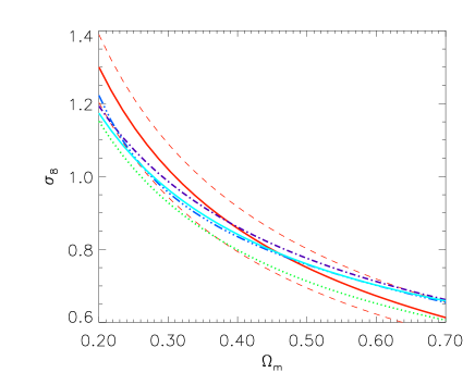
Figure 7: The normalization $\sigma_{8}$ for flat cosmologies with shape parameter fixed at $\Gamma=0.23$ as derived here (solid,red ) with 1–$\sigma$ limits (dashed red lines), compared with the fits from Viana & Liddle [Viana & Liddle 1999] (dot-dashed dark blue line), Wang & Steinhardt[Wang & Steinhardt 1998] (blue 3 dots-dashed), Eke et al. [Eke et al. 1996] (dotted green), and Borgani et al.[Borgani et al. 1999] (cyan).

In earlier cluster samples the shape of the temperature function was not obviously well fit by the theoretical predictions. Much of this discrepancy has now disappeared thanks to better data. The question remains however as to how much the shape of the temperature function affects the fit, rather than for example the overall amplitude at some intermediate temperature. To address this we have calculated $\sigma_{\rm Cl}$ for flat cosmologies by matching the observed $n({>}\,kT_{\rm X})$ for $T_{\rm X}=6\,$keV. We found values 2.5–4.5 per cent lower than fitting to the whole temperature function for $T_{\rm X}>3.5\,$keV. Thus the shape of the temperature function is being used in the fit, and shifts the best fitting $\sigma_{\rm Cl}$ by a small, but non-negligible amount.

In Fig. 7 we compare our results with those of Viana & Liddle [Viana & Liddle 1999] and others for flat cosmologies as a function of $\Omega_{\rm M}$. While the Viana & Liddle [Viana & Liddle 1999] best fit is within our error bars, the shape of the two curves is quite different. This discrepancy can be traced to a number of factors: a newer data compilation; our likelihood fit to the entire cluster data; our use of the Sheth & Tormen [Sheth & Tormen 1999] universal mass function rather than the PS theory; not integrating over formation redshifts; different $M{-}T$ normalization and scatter; and different sources of errors (in particular Viana & Liddle 1999 included errors in $\Gamma$).

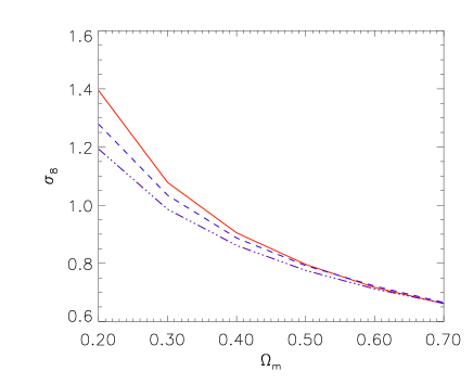
Figure 8: The normalization $\sigma_{8}$ for flat cosmologies with $\Gamma=0.23$ as derived here (solid red line) but with $\beta=1.17$, compared with the Viana & Liddle [Viana & Liddle 1999] results (dark blue dot-dashed line) and also compared with their approach but without the integration over formation redshift (blue dashed line).

We found a relatively symmetric error bar on our final results for $\sigma_{\rm Cl}$ and $\sigma_{8}$, while Viana & Liddle [Viana & Liddle 1999] had a very asymmetric error. It appears that this is mainly due to their assumed skew distribution for $\Gamma$. Another important difference is that Viana & Liddle [Viana & Liddle 1999] adopted a lower value of $\beta$ with respect to ours. If we chose $\beta=1.17$, we would find the same normalization at high $\Omega_{\rm M}$ (see Fig. 8). Approximately half of the discrepancy at lower $\Omega_{\rm M}$ comes from the fact that we have not integrated over ‘formation’ redshift, while Viana & Liddle [Viana & Liddle 1999] included such an integration (see Fig. 8). We argued in §2 that including such an integration in addition to the scatter in the $M{-}T$ relation was effectively double counting some of the scatter.

Use of the Sheth & Tormen [Sheth & Tormen 1999] or Jenkins et al. [Jenkins et al. 2001] mass function, rather than PS, lowers our results by 4–8 per cent (depending on $\Omega_{\rm M}$). Note that the overall effect of the different mass function may depend on redshift, so that if formation redshift is integrated over then the discrepancy may even be in the other direction.

A major source of theoretical uncertainty remains the value and distribution of $\beta$ in the $M{-}T$ relation of Eq. (13). We show in Fig. 9 how $\sigma_{\rm Cl}$ changes as $\beta$ is scanned from 0.9 to 1.5 (with no systematic error) in our reference model with $\Omega_{\rm M}=0.3$ and $\Omega_{\Lambda}=0.7$. It is clear that a better estimate of the $M\,{-}\,T$ relation would greatly reduce the errors on $\sigma_{\rm Cl}$. It is also clear that to obtain an unbiased estimate of $\sigma_{\rm Cl}$ it is essential to use an appropriate central value and error on $\beta$, which is why we have included both a statistical and ‘systematic’ error in our fits (see also Table 6).

Figure 9: The largely $\Gamma$-independent normalization $\sigma(R_{\rm Cl})$ for different values of $\beta$ in the $M{-}T$ relation. The error bars indicate the standard deviation of $\sigma(R_{\rm Cl})$ arising from all uncertainties except for the systematic error in $\beta$, which is set to zero here. Our adopted central value of $\beta$ is 1.3.

An estimate of the uncertainty introduced by various factors is shown in Table 6. To obtain the estimates of error budget in this table we ran our code with the sources of errors described in the first column. The first case for example is the complete calculation, with all sources of error included. The second case has only the statistical uncertainty in the $M{-}T$ relation, while the uncertainty in the value of the cluster temperature and the systematic scatter in the $M{-}T$ relation were not used. The other cases show what happens with one or other source of uncertainty excluded. The mean quoted is the mean of the distribution obtained in each case, while the the errors are obtained by integrating the normalized distribution until 34 per cent of the area is reached on each side of the mean.

We find that our uncertainty in $\sigma_{8}$ is dominated by systematics in the $M{-}T$ relation (see also Voit 2000). The statistical scatter in the $M{-}T$ relation has an almost negligible effect on the central value and the error. The temperature errors themselves give a skewed distribution to $\sigma_{8}$, but this effect is sub-dominant.

6 Conclusions

Table 6: For a flat cosmology with $\Omega_{\rm M}=0.3$ we estimate how each source of uncertainty affects the mean and the error of our $\sigma_{\rm Cl}$ estimates. $M{-}T|_{\rm sys}$ and $M{-}T|_{\rm stat}$ represent the systematic and statistical errors in the $M{-}T$ relation, while $T$ represents the error in the temperature of the clusters. The $+1\sigma$ and $-1\sigma$ limits are found from integrating the distribution of 1000 Monte Carlos in each case.

Source of error	mean $\sigma(R_{\rm Cl})$	$+1\sigma$	$-1\sigma$
all	0.581	0.049	0.050
$M{-}T|_{\rm sys}$	0.575	0.047	0.047
$M{-}T|_{\rm stat}$	0.570	0.002	0.002
$T$	0.586	0.005	0.018

The local abundance of rich clusters of galaxies currently provides one of the strongest constraints on the normalization of the present day dark matter power spectrum on a scale of ${\sim}\,10\,$Mpc. While there have been numerous detailed studies of this constraint in the past, recent developments in both theory and observation have made it worthwhile to revisit this quantity.

We have calculated the constraint on $\sigma_{8}$ arising from a new local sample of X-ray clusters with ASCA temperatures. We have incorporated the universal mass function determined from recent large N-body simulations, which is sufficiently different from the PS theory that the cosmological constraints inferred from cluster abundances change. We tried to carefully define the relation between mass and X-ray temperature for galaxy clusters, based on the results of many different hydrodynamical simulations. Another major difference with previous work was that we performed all the comparisons at the ‘observed epoch’ rather than carrying out an integration over ‘formation times’. We also considered general combinations of $\Omega_{\rm M}$ and $\Omega_{\rm\Lambda}$, including closed models. Our results are best presented in terms of a normalization at the characteristic scale for our sample, $R_{\rm Cl}$, where the normalization is largely independent of the power spectrum shape.

In the near future we anticipate a dramatic increase in our knowledge of the cosmological parameters from CMB anisotropy missions. In particular it has been forecast [Eisenstein, Hu & Tegmark 1999] that MAP will be able to determine $\sigma_{8}$ to 14 per cent, at the same time as constraining a suite of other parameters. The cluster abundance constraint is currently uncertain only at the ${\sim}\,10$ per cent level, and so certainly is a pivotal limit on models – it is also an entirely independent constraint (at low $z$, in the mildly non-linear regime) compared with the CMB determinations (derived from the purely linear regime at $z\simeq 1000$). The uncertainty in the derived $\sigma_{8}$ could be dramatically reduced with improvement in the $M{-}T$ relation, as well as through new X-ray data coming from Chandra and XMM-Newton.

Future X-ray surveys, which go much fainter will lead to an increase in the size and quality of the X-ray data. We showed in Fig. 4 that there is lots of volume that was not probed at, say, $5\,$keV. For example the ROSAT Bright Survey [Schwope et al. 2000] contains an approximately complete flux-limited sample of 302 clusters at $|b|\,{>}\,30^{\circ}$, most of them lying at low redshift, which would be an excellent data-base if they all had good temperature estimates. More important than just increasing the precision of the X-ray temperature measurements is an increase in the quality of data, for the purposes of more fully understanding the comparison with models. Better spatial and spectral information from X-ray clusters should allow more reliable estimates for the value of $T_{\rm X}$ which is most appropriate for comparing with the simulations. In a similar vein, improved optical studies of lensing and velocity dispersions could improve mass determinations for individual clusters.

The major improvement will come through a more precise mass-temperature relation for X-ray clusters. This will require both the improved data which we can foresee from Chandra and XMM-Newton, and improvements in modelling the gas physics relevant for understanding the X-ray properties of clusters. Eventually we imagine that the data will be fit more directly to much more ambitious simulations – this will be extremely difficult in practice, since a wide range of scales needs to be modelled simultaneously. In the meantime the piece-meal approach we have taken here will continue to be useful. With each of the ingredients, particularly the mass-temperature relation, improving with time, the cluster abundance will continue to be a strong constraint on the normalization of dark matter fluctuations on the ${\sim}\,10\,$Mpc scale.

ACKNOWLEDGMENTS

EP and DS were supported by the Canadian Natural Sciences and Engineering Research Council, and MW by the US National Science Foundation and a Sloan Fellowship. EP is a National Fellow of the Canadian Institute for Theoretical Astrophysics. We would like to thank the Institute for Theoretical Physics, Santa Barbara for their hospitality while some of this work was carried out. We are indebted to Alain Blanchard, Stefano Borgani, Patrick Henry, Andrew Liddle, Maxim Markevitch and David Weinberg for providing useful comments on an early version of the manuscript. This research has made use of the NASA/IPAC Extragalactic Database (NED) which is operated by the Jet Propulsion Laboratory, California Institute of Technology, under contract with the National Aeronautics and Space Administration.

References

- [Allen 1998] Allen S.W., 1998, MNRAS, 296, 392
- [Bahcall & Cen 1993] Bahcall N., Cen R., 1993, ApJ, 407, L49
- [Balogh et al. 1999] Balogh M.L., Babul A., Patton D.R., 1999, MNRAS, 307, 463
- [Böhringer et al. 2001] Böhringer H., Schuecker P., Guzzo L., Collins C.A., Voges W., et al., 2001, A&A, in press, astro-ph/0012266
- [Bardeen et al. 1986] Bardeen J.M., Bond J.R., Kaiser N., Szalay A.S., 1986, ApJ, 304, 15
- [Blanchard et al. 2000] Blanchard A., Sadat R., Bartlett J.G., Le Dour M., 2000, A&A, 362, 809
- [Bond & Myers 1991] Bond J.R., Myers S.T., 1991, Trends in Astroparticle Physics, eds. D. Cline, R. Peccei, World Scientific, Singapore, p. 262
- [Bond & Myers 1996] Bond J.R., Myers S.T., 1996, ApJS, 103, 63
- [Borgani et al. 1999] Borgani S., Rosati P., Tozzi P. Norman C., 1999, ApJ, 517, 40
- [Bryan & Norman 1998] Bryan G.L., Norman M.L., 1998, ApJ, 495, 80
- [Carlberg et al. 1996] Carlberg R.G., Yee H.K.C., Ellingson E., Abraham R., Gravel P., et al., 1996, ApJ, 462, 32
- [Carroll, Press & Turner 1992] Carroll S.M., Press W.H., Turner E.L., ARAA, 30, 499
- [Cavaliere, Menci & Tozzi 1999] Cavaliere A., Menci N., Tozzi P., 1999, MNRAS, 308, 599
- [Cohn 1999] Cohn J., 1999, Astrophys. & Space Science, 259, 213.
- [Colafrancesco et al. 1997] Colafrancesco S., Mazzotta P., Vittorio N., 1997, ApJ, 488, 566
- [David 1993] David L.P., Slyz A., Jones C., Forman W., Vrtilek S.D., et al. 1993, ApJ, 412, 479
- [Davis et al. 1985] Davis M., Efstathiou G., Frenk C.S., White S.D.M., 1985, ApJ, 292, 371
- [de Grandi et al. 1999] de Grandi S., Böhringer H., Guzzo L., Molendi S., Chincarini G., et al. 1999, ApJ, 514, 148
- [Donahue & Voit1999] Donahue M., Voit G.M., 1999, ApJ 523, L137
- [Ebeling et al. 1996] Ebeling H., Voges W., Böhringer H., Edge A.C., Huchra J.P., et al. 1996, MNRAS, 281, 799
- [Ebeling et al. 1998] Ebeling H., Edge A.C., Böhringer H., Allen S.W., Crawford C.S., et al. 1998, MNRAS, 301, 881
- [Edge et al. 1990] Edge A., Stewart G.C., Fabian A.C., Arnaud K.A., 1990, MNRAS, 245, 559
- [Eisenstein & Hu 1999] Eisenstein D., Hu W., 1999, ApJ, 511, 5
- [Eisenstein, Hu & Tegmark 1999] Eisenstein D., Hu W., Tegmark M., 1999, ApJ, 518, 2
- [Eisenstein & Zaldarriaga 2001] Eisenstein D., Zaldarriaga M., 2001, ApJ, 546, 2 [astro-ph/9912149]
- [Eke et al. 1996] Eke V., Cole S., Frenk C.S., 1996, MNRAS, 282, 263
- [Eke et al. 1998] Eke V., Cole S., Frenk C.S., Henry P.J., 1998, MNRAS, 298, 1145
- [Eke et al. 1998] Eke V., Navarro J.F., Frenk C.S., 1998, ApJ, 503, 569
- [Evrard 1989] Evrard A.E., 1989, ApJ, 341, L71
- [Evrard et al. 1996] Evrard A.E., Metzler C., Navarro J.F., 1996, ApJ, 469, 494
- [Finoguenov et al. 2001] Finoguenov A., Arnaud M., David L.P., 2001, ApJ, in press [astro-ph/0009007]
- [Frenk et al. 1990] Frenk C.S., White S.D.M., Efstathiou G., Davis M., 1990, ApJ, 351, 10
- [Frenk et al. 1999] Frenk C.S., White S.D.M., Bode P., Bond J.R., Bryan G.L., et al. 1999, ApJ, 525, 554
- [Gardner et al. 2000] Gardner J.P., 2000, preprint [astro-ph/0006342]
- [Girardi et al. 1998a] Girardi M., Giuricin G., Mardirossian F., Mezzetti M., Boschin W., 1998a, ApJ, 505, 74
- [Girardi et al. 1998b] Girardi M., Borgani S., Giuricin G., Mardirossian F., Mezzetti M., 1998b, ApJ, 506, 45
- [Girardi et al. 2000] Girardi M., Borgani S., Giuricin G., Mardirossian F., Mezzetti M., 2000, ApJ, 530, 62
- [Governato et al. 1999] Governato F., Babul A., Quinn T., Tozzi P., Baugh C.M., et al., 1999, MNRAS, 307, 949
- [Hamilton 2001] Hamilton A.J.S., 2001, MNRAS, 322, 419 [astro-ph/0006089]
- [Hanami 1993] Hanami H., 1993, ApJ, 415, 42
- [Heath 1977] Heath D.J., 1977, MNRAS, 179, 351
- [Henry 2000] Henry J.P., 2000, ApJ, 534, 565
- [Henry & Arnaud 1991] Henry J.P., Arnaud K.A., 1991, ApJ, 372, 410
- [Horner, Mushotsky & Scharf 1999] Horner D.J., Mushotsky R.F., Scharf C.A., 1999, ApJ, 520, 78
- [Irwin & Bregman 2000] Irwin J.A, Bregman J.N., 2000, ApJ, 538, 543
- [Irwin, Bregman & Evrard 1999] Irwin J.A, Bregman J.N., Evrard A.A., 1999, ApJ, 519, 518
- [Jenkins et al. 2001] Jenkins A., Frenk C.S., White S.D.M., Colberg J.M., Cole S., Evrard A.E., Yoshida N., 2001, MNRAS, 321, 371 [astro-ph/0005260]
- [Kaiser 1991] Kaiser N., 1991, ApJ, 383, 104
- [Kitayama & Suto 1997] Kitayama T., Suto Y., 1997, ApJ, 490, 557
- [Lahav et al. 1991] Lahav O., Rees M.J., Lilje P.B., Primack J.R., 1991, MNRAS, 251, 128
- [Liddle & Lyth 2000] Liddle A., Lyth D., 2000, Cosmological Inflation and Large-Scale Structure, Cambridge University Press, Cambridge.
- [Lilje 1992] Lilje P.B., 1992, ApJ, 386, L33
- [Markevitch 1998] Markevitch M., 1998, ApJ, 504, 27
- [Mathiesen 2000] Mathiesen B.F., 2000, MNRAS, submitted [astro-ph/0012117]
- [Mathiesen & Evrard 2001] Mathiesen B.F. & Evrard A.E., 2001, ApJ, 546, 100 [astro-ph/0004309]
- [Mohr & Evrard 1997] Mohr J.J., Evrard A.E., 1997, ApJ, 491, 38
- [Molnar & Jahoda 2000] Molnar S.M., Jahoda K., 2000, [astro-ph/0002270]
- [Navarro et al. 1996] Navarro J.F., Frenk C.S., White S.D.M., 1996, ApJ, 462, 563
- [Nevalainen, Markevitch & Forman 2000] Nevalainen J., Markevitch M., Forman W., 2000, ApJ, 532, 694 [astro-ph/9911369]
- [Ostriker & Steinhardt 1995] Ostriker J.P., Steinhardt P.S., 1995, Nature, 377, 600
- [Oukbir & Blanchard 1992] Oukbir J., Blanchard A., 1992, A&A, 262, L21
- [Peacock 1999] Peacock J.A., 1999, Cosmological Physics, Cambridge University Press, Cambridge.
- [Peebles 1993] Peebles, P.J.E., 1993, Principles of Physical Cosmology, Princeton University Press, Princeton, chapter 25.
- [Pen 1998] Pen U.-L., 1998, ApJ, 498, 60
- [Press & Schechter 1974] Press W.H., Schechter P., 1974, ApJ, 187, 452
- [Reiprich & Böhringer 1999] Reiprich T.H., Böhringer H., 1999, 19th Texas Symposium on Relativistic Astrophysics and Cosmology, ed. J. Paul, T. Montmerle, E. Aubourg, in press
- [Schwope et al. 2000] Schwope A.D., Hasinger G., Lehmann I., Schwarz R., Brunner H. et al. 2000, Astron. Nach., 321, 1
- [Sheth, et al. 2001] Sheth R.K., Mo H.J., Tormen G., 2001, MNRAS, 323, 1 [astro-ph/9907024]
- [Sheth & Tormen 1999] Sheth R.K., Tormen G., 1999, MNRAS, 308, 119
- [Smail et al. 1997] Smail I., Ellis R.S., Dressler A., Couch W.J., Oemler A., et al., 1997, ApJ, 479, 70
- [Struble & Rood 1999] Struble M.F., Rood H., 1999, ApJS, 125, 35
- [Tanaka, Inoue & Holt 1994] Tanaka Y., Inoue H., Holt S.S., 1994, PASJ, 46, L37
- [Thomas et al. 2000] Thomas P.A., Muanwong O., Pearce F.R., Couchman H.M.P., Edge A.C., et al., submitted to MNRAS [astro-ph/0007348]
- [Tittley & Couchman 2000] Tittley E.R., Couchman H.M.P., 2000, submitted to MNRAS [astro-ph/9911365]
- [Viana & Liddle 1996] Viana P.T.P., Liddle A., 1996, MNRAS, 281, 323
- [Viana & Liddle 1999] Viana P.T.P., Liddle A., 1999, MNRAS, 303, 535
- [Voit 2000] Voit G.M., 2000, ApJ, 543, 113
- [Wang & Steinhardt 1998] Wang L., Steinhardt P.J., 1998, ApJ, 508, 483
- [White 2000] White D.A., 2000, MNRAS, 312, 663
- [White & Buote 2000] White D.A., Buote D.A., 2000, MNRAS, 312, 649
- [White et al. 1997] White D.A., Jones C., Forman W., 1997, MNRAS, 292, 419
- [White & Scott 1996] White M., Scott D., 1996, ApJ, 459, 415
- [White, Scott & Pierpaoli 2000] White M., Scott D., Pierpaoli E., 2000, ApJ, 545, 1
- [White, Efstathiou & Frenk 1993] White S.D.M., Efstathiou G., Frenk C.S., 1993, MNRAS, 262, 1023
- [Wu et al. 1998] Wu X.-P., Chiueh T., Fang L.-Z., Xue Y.-J., 1998, MNRAS, 301, 861
- [Xue & Wu 2000] Xue Y.-J., Wu X.-P., 2000, ApJ, 538, 65
- [Yoshikawa, Jing & Suto 2000] Yoshikawa K., Jing Y.P., Suto Y., 2000, ApJ, 535, 593