Photoevaporating flows from the cometary knots in the Helix nebula (NGC 7293)

Abstract

We explain the H$\alpha$ emission of the cometary knots in the Helix Nebula (NGC 7293) with an analytical model that describes the emission of the head of the globules as a photoevaporated flow produced by the incident ionizing radiation of the central star. We compare these models with the H$\alpha$ emission obtained from the HST (Hubble Space Telescope) archival images of the Helix Nebula. From a comparison of the H$\alpha$ emission with the predictions of the analytical model we obtain a rate of ionizing photons from the central star of about $\rm 5\times 10^{45}\ s^{-1}$, which is consistent with estimates based on the total H$\beta$ flux of the nebula. We also model the tails of the cometary knots as a photoevaporated wind from a neutral shadow region produced by the diffuse ionizing photon field of the nebula. A comparison with the HST images allows us to obtain a direct determination of the value of the diffuse ionizing flux. We compare the ratio of diffuse to direct stellar flux as a function of radius inside an HII region with those obtained from the observational data through the analytical tail and head wind model. The agreement of this model with the values determined from the observations of the knots is excellent.

1. Introduction

The small scale structure of the Planetary Nebula (PN) known as the Helix Nebula (NGC 7293, PK 36-57^∘1) is characterized by many thousands of small knots. These knots (which were first reported by Vorontsov–Velyaminov 1968) have a cometary shape, with their tails pointing away from the central source. Groundbased work (Meaburn et al. 1992, 1996, 1998) and Wide Field and Planetary Camera HST observations (O’Dell & Handron 1996; O’Dell & Burkert 1997; Burkert & O’Dell 1998) revealed a multitude of spatially resolved knots, about 3500, with highly symmetric appearance. The knots have also been detected in CO (Huggins et al. 1992) and, at least outside the main nebula, in C I (Young et al. 1997).

This PN is one of the closest to us with a parallax distance of 213 pc (Harris et al. 1997). Other methods have been applied to determine the distance to this PN, giving values ranging from 120 to 400  pc. Optical images show a complicated morphology characterized by a helical structure in H$\alpha$ and [N II] and a more elliptical shape in [O III]. The deprojection of these images has proven to be difficult, with suggestions of both elliptical/toroidal shapes and bipolar ones (Meaburn & White 1982) being made. O’Dell (1998) has suggested that the ionized region is a disk.

The central star is very hot and has a low luminosity, indicating that it is well down the cooling track of its post-AGB evolution. The temperature of the central star of the Helix has been measured by the H$\beta$ Zanstra method to be $\simeq 1.2\times 10^{5}\,\rm{K}$ (Górny, Stasińska & Tylenda 1997).

The high effective temperature combined with the fairly low luminosity and the large size of the PN , about 0.5 pc in diameter at a distance of 213 pc, leads to a complicated ionization structure with co-existing regions of high and low ionization character (O’Dell 1998; Henry, Kwitter & Dufour 1999). The low luminosity of the star also implies a very low density wind, making it virtually undetectable. However, with its expected high velocity ($v_{\infty}\simeq 6000$ km s^-1 if radiation driven) it could still have a dynamical effect on the PN structure.

The measured densities in the nebula are low, about 60 cm^-3 (O’Dell 1998), in contrast with the densities derived for the neutral/molecular globules, $n_{\rm knot}\sim 10^{6}$ cm^-3 (O’Dell & Handron 1996). This leads to the curious result that a substantial fraction of the mass of the PN is in the form of these neutral globules. The aspherical shape of the PN is also found in the distribution of the knots and in the large scale CO emission. Meaburn et al. (1998) have shown that the knots follow the same velocity distribution as the CO, although at a lower typical expansion velocity. Young et al. (1999) found the deprojected expansion velocities of the knots and the CO ring to be 19 and 29 $\rm km~{}s^{-1}$, respectively.

Some other authors have treated the photoevaporation of clumps in an ionizing radiation field. Bertoldi & McKee (1990) developed an approximate analytic theory of the evolution of a photoevaporating cloud exposed to the ionizing radiation of a newly formed star, finding an equilibrium cometary cloud configuration. Johnstone, Hollenbach & Bally (1998) modelled the photoevaporation of dense clumps of gas by an external source of ultraviolet radiation including thermal and dynamical effects. Mellema et al. (1998) study the evolution of dense neutral clumps located in the outer parts of a planetary nebula (like the Helix nebula).

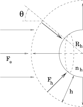
Figure 1.— Schematic diagram of the cometary head. $F_{h}$ is the incident flux at the surface of the neutral knot, and $R_{h}$ and $n_{h}$ are the radius and the density of the neutral knot (respectively).

2. Analytical model for the photoevaporated flux of the cometary knots

Let us discuss a simple, analytical model for cometary knots embedded in a Planetary Nebula (PN). First, we derive some expressions that relate the ionizing stellar flux and the particle flux of the photoevaporated wind in a similar way to Mellema et al. (1998) to find the $\rm H\alpha$ emission for the cometary heads. Cantó et al. (1998) proposed the idea of the tails as neutral shadow regions behind the clumps, and studied the complex time-evolution of the resulting flow. In this paper, we model the tails behind the Helix clumps as a cylinder of neutral material being photoionized by the diffuse ionizing flux of the nebula.

2.1. A model for the cometary head

Let us consider the problem of a hemispherical, neutral knot of radius $R_{h}$ which is being photoionized by the radiative field emitted by the central star of the ionized nebula. A schematic diagram of this configuration is shown in Figure 1.

A fraction of the stellar flux arrives at the knot surface, photoionizing the neutral knot material and feeding a photoevaporated flow. The remaining ionizing photons are absorbed in this photoevaporated flow. The neutral knot is being photoevaporated, but we consider a quasi-steady state in which the radius of the knot $R_{h}$ is almost constant with time. The incident flux at the knot surface is :

$$F_{h}(\theta)=n_{h}(\theta)~{}v(R_{h})\,,$$

where $F_{h}$ is the flux of ionizing photons incident normal to the knot surface (per unit area and time), $n_{h}$ and $v(R_{h})$ are the density and the velocity of the photoevaporated wind at the knot surface . We note that the rate of photoionizations depends on the angle of incidence $\theta$ (see Figure 1), having a maximum value in the front of the cometary head.

In order to obtain the density profile, we consider the conservation of particles in the photoevaporated wind :

$$R^{2}n(R,\theta)v(R)=R_{h}^{2}n_{h}(\theta)v(R_{h})\,,$$

where $R$ is the radius directed outwards from the knot.

We assume that the ionization front is thin compared with the effective thickness $h$ of the ionized flow and that $h$ in turn is small compared with $R_{h}$. In this case, if all diffuse photons are absorbed “on-the-spot”, the photoionization balance is given by

$$F_{\star}~{}\cos(\theta)\simeq F_{h}(\theta)+h~{}n_{h}^{2}(\theta)~{}\alpha_{B}\,,$$

where $\alpha_{B}$ is the case B recombination coefficient of hydrogen, which is assumed to be constant with position. The flow thickness $h$ is defined by :

$$h\equiv\omega~{}R_{h}\,,$$

where the parameter $\omega$ is defined through the relation :

$$\omega~{}n_{h}^{2}~{}R_{h}\equiv\int_{R_{h}}^{\infty}n^{2}(r)~{}dr\,.$$

This parameter $\omega$ depends on the density profile of the photoevaporated wind. For a D-critical ionization front $(v(R_{h})=c_{i}$, where $c_{i}$ is the isothermal sound speed of the ionized gas), $\omega\simeq 0.1$ (Henney & Arthur 1998). From equations (1-5) we then obtain a relation between the ionizing flux from the central star $F_{\star}$, and the incident flux at the knot surface $F_{h}(\theta)$ :

$$F_{\star}~{}\cos(\theta)\simeq F_{h}(\theta)+F_{h}^{2}(\theta)~{}{\omega~{}R_{h}~{}\alpha_{B}\over{c_{i}^{2}}}\,,$$

The term on the left is the ionizing stellar flux as a function of the angle of incidence, the first term on the right is the incident ionizing flux on the knot surface that produces the photoionizations of the neutral material and the second term is the flux absorbed in the photoevaporated wind. If we define :

$$\xi_{h}\equiv{c_{i}^{2}\over{R_{h}~{}\omega~{}\alpha_{B}}}\,,$$

equation (6) can be written as  :

$$F_{\star}~{}\cos(\theta)\simeq F_{h}(\theta)+{F_{h}^{2}(\theta)\over\xi_{h}}\,,$$

We can see from equation (8) that it is possible to find the incident flux $F_{h}(\theta)$ as a function of the ionizing flux $F_{\star}$ solving the quadratic equation to obtain :

$$F_{h}(\theta)\simeq{\xi_{h}\over 2}\left[\left({4~{}F_{\star}~{}\cos(\theta)\over\xi_{h}}+1\right)^{1/2}-1\right]\,.$$

We find two different limiting situations :

If $\xi_{h}/\cos(\theta)<<F_{\star}$ we have the ^′′Recombination Dominated Regime ^′′ in which the fluxes are related by the expression :

$$F_{h}(\theta)\approx\sqrt{\xi_{h}~{}F_{\star}~{}\cos(\theta)}\,,$$

In this case, an important fraction of the ionizing flux is absorbed in the photoevaporated wind and only a small fraction of the stellar flux arrives at the knot surface. The recombinations in the column beyond $R_{h}$ mainly balance the stellar flux.

If $\xi_{h}/\cos(\theta)>>F_{\star}$ we have the ^′′Flux Dominated Regime ^′′, in which :

$$F_{h}(\theta)\approx F_{\star}~{}\cos(\theta)\,,$$

In this regime almost all the stellar flux arrives at the knot surface and there is no absorption in the photoevaporated flow. The paticle flux at $R_{h}$ is roughly equal to the stellar flux.

In order to compute the total rate of $\rm H{\alpha}$ photons emitted by the head of a cometary knot, assuming $\omega\ll 1$ we have to evaluate the integral :

$$S_{\rm H\alpha}\simeq\int_{0}^{\pi/2}2~{}\pi~{}R_{h}^{2}~{}\alpha_{\rm H\alpha}~{}n^{2}_{h}(\theta)~{}\sin(\theta)~{}\omega~{}R_{h}~{}d\theta\,,$$

where $\alpha_{\rm H{\alpha}}$ is the effective $\rm{H{\alpha}}$ recombination coefficient.

Taking into account the angular dependence of the density profile we can integrate (12) to obtain the $\rm H\alpha$ emission of the cometary heads :

$$S_{\rm{H\alpha}}\simeq\pi R_{h}^{2}{\alpha_{\rm H\alpha}\over\alpha_{B}}F_{\star}\left\{1+{\xi_{h}\over F_{\star}}-{\xi_{h}^{2}\over{6F_{\star}^{2}}}\left[\left(1+{4F_{\star}\over\xi_{h}}\right)^{3/2}-1\right]\right\}\,.$$

The term in curly brackets is the fraction of incident ionizing photons that are absorbed in the photoevaporating flow before reaching the ionization front. It is only this fraction of the incident photons that are reprocessed into H$\alpha$ radiation. If we know the size of the knot $R_{h}$ and the H$\alpha$ emission $S_{\rm H{\alpha}}$ we can use equation (13) to estimate the stellar flux.

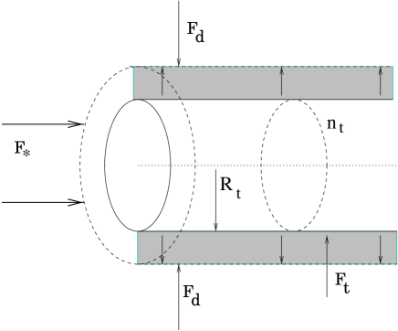
Figure 2.— Schematic diagram of the cometary tail. $F_{t}$ is the incident flux at the surface of the neutral cylinder, $F_{d}$ is the diffuse flux (produced by the surrounding nebula), and $R_{t}$ and $n_{t}$ are the radius and the density of the neutral tail (respectively).

2.2. A model for the cometary tail

For the cometary tail, we consider the problem of a cylinder of neutral material behind the cometary head being photoionized by the diffuse flux of the nebula. A schematic diagram of this configuration is shown in Figure 2. If we assume that the radius of the cometary head is much smaller than the distance to the source we can consider the shadow region to have polar symmetry. This cylindrical shadow does not receive direct stellar radiation. We therefore have :

$$F_{d}=F_{t}+\omega~{}R_{t}~{}n_{t}^{2}~{}\alpha_{B}\,,$$

where $F_{d}$ is the diffuse ionizing flux of the surroundings, $F_{t}$ is the incident flux at the tail surface and the second term on the right represents the absorptions in the photoevaporated wind of the cometary tail.

The incident flux at the neutral surface of the tail is related to the density $n_{t}$ at the base of the cylindrical wind through :

$$F_{t}=n_{t}~{}c_{i}\,,$$

Defining the parameter :

$$\xi_{t}\equiv{{c_{i}^{2}}\over{\omega~{}\alpha_{B}~{}R_{t}}}\,,$$

and subsituting equations (15-16) in (14) one obtains :

$$F_{d}=F_{t}+{F_{t}^{2}\over\xi_{t}}\,.$$

In order to obtain the total number of $\rm{H{\alpha}}$ photons emitted by the tails of the cometary knots, we assume that the H${\alpha}$ emitting region has a cylindrical section with a thickness $h\equiv\omega~{}R_{t}$. The number of H$\alpha$ photons emitted per unit time and per unit length of this cylinder is :

$${S_{\rm H{\alpha}}\over{\Delta l}}=2~{}\pi~{}R_{t}~{}\omega~{}R_{t}~{}n^{2}_{t}~{}\alpha_{\rm H{\alpha}}\,,$$

and as a function of the parameter $\xi_{t}$ the $\rm H\alpha$ emission is :

$${S_{\rm H{\alpha}}\over{\Delta l}}=2~{}\pi~{}R_{t}~{}{\alpha_{\rm H{\alpha}}\over\alpha_{B}}~{}{F_{t}^{2}\over\xi_{t}}\,,$$

where $\Delta l$ is a unit of length along the cylindrical tail. If we combine equations (17) and (19) we can calculate the diffuse ionizing flux as a function of the H${\alpha}$ emission per unit length and the radius of the cylinder :

$$F_{d}={{S_{\rm H{\alpha}}/{\Delta l}}\over{2~{}\pi~{}R_{t}}}~{}{{\alpha_{B}}\over{\alpha_{\rm H{\alpha}}}}+\left[{{S_{\rm H{\alpha}}/{\Delta l}}\over{2~{}\pi~{}R_{t}}}~{}{{\alpha_{B}}\over{\alpha_{\rm H{\alpha}}}}~{}\xi_{t}\right]^{1/2}\,.$$

2.3. Diffuse ionizing field inside an H II region

As well as the radial ionizing radiation field from the Helix central star, there will also be a diffuse ionizing radiation field, principally due to ground level recombinations of hydrogen in the nebula, plus smaller contributions from helium recombinations and the scattering of stellar radiation by dust grains. For the purposes of calculating the properties of the knot tails, the important quantity is the lateral flux of the diffuse field, which is the flux incident on the surface of an opaque, radially aligned, thin cylinder.

In the “on-the spot” (OTS) approximation, in which all diffuse ionizing photons are assumed to be reabsorbed by neutral H very close to their point of emission, the diffuse flux, $F_{d}$, across any opaque surface is related to the stellar flux, $F_{*}$, at the same position by (Henney 2000)

$$\beta_{\rm OTS}\equiv\frac{F_{d}}{F_{*}}=\frac{\alpha_{1}}{4\alpha_{B}\kappa}\,,$$

where $\alpha_{1}$ and $\alpha_{B}$ are, respectively, the H recombination rates to the ground level and to all excited levels and $\kappa=\bar{\sigma}_{d}/\bar{\sigma}_{*}$, where $\bar{\sigma}_{d}$ is the mean photoionization cross-section averaged over the diffuse ionizing spectrum and $\bar{\sigma}_{*}$ is the same quantity averaged over the stellar spectrum. Henney (2000) presents detailed calculations, in which the OTS assumption is relaxed, for the lateral diffuse flux in two simplified geometries: a classical filled-sphere homogeneous Strömgren H II region, and a hollow cavity H II region with the ionized gas concentrated in a thin spherical shell. It is found that in both cases the value of $\beta(=\frac{F_{d}}{F_{*}})$ is much smaller than $\beta_{OTS}$ at small radii. It is because at small radi, $F_{\star}$ gets huge ($r^{-2}$) but $F_{d}$, which is proportional to the recombination rate times a path length, plateaus to a more or less constant value. In the thin-shell case, $\beta$ remains at a low value throughout the interior of the cavity, only becoming comparable to $\beta_{\rm OTS}$ at the position of the shell. In the filled-sphere case, on the other hand, for the relatively high values of $\kappa$ appropriate for the Helix knots (see below), $\beta$ rises to $\simeq\beta_{\rm OTS}$ at a fractional radius of $\simeq 0.5$ and is roughly constant thereafter.

The stellar ionizing radiation field is much harder than the diffuse field, while the photoionization cross-section declines rapidly with frequency above the ionization threshold. Hence, the ratio of mean cross-sections, $\kappa$, for the diffuse and stellar fields is larger than unity. Including the H and He⁰ recombination spectrum gives $\bar{\sigma}_{d}\simeq 0.75\sigma_{0}$, where $\sigma_{0}$ is the threshold cross-section and $\rm{He/H}=0.13$ (O’Dell 1998; Henry, Kwitter & Dufour 1999) has been assumed.

The temperature of the central star of the Helix has been measured by the H$\beta$ Zanstra method to be $\simeq 1.2\times 10^{5}\,\mathrm{K}$ (Górny, Stasińska & Tylenda 1997). A further constraint on the stellar spectrum is the observation (O’Dell 1998) that the He⁺⁺ zone in the nebula is roughly half the radius of the He⁺ zone, implying that roughly 10$\%$ of the ionizing photons have frequencies higher than the He⁺ ionization limit. Model atmospheres for compact hot stars (Rauch 1997) that are consistent with these constraints have photon spectra $L_{\nu}/h\nu$ that are flat or rising between the H and He⁺ ionization limits, implying a value of $\bar{\sigma}_{*}\simeq 0.17\sigma_{0}$.

Hence, $\kappa\simeq 4.5$ is appropriate for the Helix knots, which implies $\beta_{\rm OTS}\simeq 0.033$ for an assumed electron temperature of $10^{4}\,{K}$. The true situation in the Helix nebula is probably intermediate between the filled-sphere and the hollow-shell case. Although O’Dell (1998) finds that the electron density is roughly constant with radius throughout the nebula, the central high-ionization “hole” has a higher temperature and hence a lower emissivity of diffuse ionizing photons. Furthermore, the geometry is more disk-like than spherical, which would tend to reduce the intensity of the diffuse field.

The radial dependence of $\beta$ in the two limiting cases is shown in Figure 3. This is compared with the observational data in section 3.3.

Figure 3.— Comparison of the Henney (2000) models to the observed values of the diffuse to direct flux ratio (crosses) as a function of the distance from the ionization front. The upper horizontal line is the OTS value and the solid line and dashed line give the variation of $\beta$ across the nebula for the filled-sphere and hollow-shell case, respectively.

3. Properties of the cometary knots

We have used the HST images from the data archive at the Space Telescope Science Institute to obtain the H$\alpha$ emission from the cometary knots in the Helix Nebula. These images are flux-calibrated using the coefficients given in O’Dell & Doi 1999. The f656n and f658n filters was selected to isolated the H$\alpha$ and [NII] emission at 658.4 nm. The [NII] emission is not much stronger than H$\alpha$, and thus it does not produce an important contamination of the H$\alpha$ observations (less than $\approx 15\%$).

Several methods have been used in order to obtain the distance to this PN (Cahn & Kaler 1971; Daub 1982; Cahn, Kaler & Stanghellini 1992; Harris et al 1997), leading to distances ranging from 120 to 400 pc. We use the value of 213 pc determined by Harris et al. (1997) from trigonometric parallax.

The comparison between the models and the observations is done for 26 knots, chosen for being relatively well isolated, and covering a range of distances to the central star.

3.1. Sizes of the knots

In order to determine the sizes of the knots, we carry out aperture photometry with a series of circular diaphragms (centred on the knots) of increasing angular radius. If one plots the flux within the aperture versus radius, for large enough radii the flux has to increase as the square of the radius (due to the presence of the bright, surrounding nebular environment). From a logarithmic plot it is then straightforward to determine the radius $R_{ext}=R_{h}+\omega R_{h}$ (see equations 4-5 and Figure 1) at which the quadratic flux vs. radius dependence first appears. In this way one then determines the value of the radius $R_{h}$ of the neutral clump.

Applying this method to the 26 chosen knots we find that there is no correlation between the size of the knots and their distance to the central star (see Figure 4). However, this could be a result of the fact that we only have a few knots, and that these knots are not necessarily representative of the true distribution of knot sizes (as they were chosen so as to be well isolated, see above). We calculate a mean radius for the knots of $<R_{h}>=(0.68\pm 0.07)~{}^{\prime\prime}$.

3.2. H$\alpha$ intensities of the cometary heads

Subtracting the background from the fluxes determined with the aperture photometry, we obtain the H$\alpha$ fluxes emitted by the knots. One can then use equation (13) to calculate the stellar ionizing flux at the position of the successive knots as a function of distance from the central star.

Table 1Location and fluxes of the cometary knots

$\alpha_{2000}$	$\delta_{2000}$a	$R_{h}~{}(^{\prime\prime})$	$S_{H\alpha}$ (s-1)	$S_{H\alpha}$ (cm-1 s-1)	$F_{*}$  (cm-2 s-1)	$F_{d}$  (cm-2 s-1)	$F_{d}/F_{\star}$
429	-860	0.73	${10.84\times 10^{39}}$	${2.96\times 10^{22}}$	${1.02\times 10^{10}}$	${1.67\times 10^{8}}$	$1.63\times 10^{-2}$
433	-853	0.69	${5.16\times 10^{39}}$	${1.60\times 10^{22}}$	${7.21\times 10^{9}}$	${1.29\times 10^{8}}$	$1.79\times 10^{-2}$
431	-844	0.66	${4.67\times 10^{39}}$	${2.53\times 10^{22}}$	${7.53\times 10^{9}}$	${1.70\times 10^{8}}$	$2.26\times 10^{-2}$
440	-848	0.73	${4.30\times 10^{39}}$	–	${5.93\times 10^{9}}$	–	–
452	-901	0.69	${3.44\times 10^{39}}$	${1.54\times 10^{22}}$	${5.74\times 10^{9}}$	${1.27\times 10^{8}}$	$2.20\times 10^{-2}$
428	-827	0.65	${2.52\times 10^{39}}$	${2.25\times 10^{22}}$	${5.31\times 10^{9}}$	${1.63\times 10^{8}}$	$3.07\times 10^{-2}$
459	-905	0.67	${3.36\times 10^{39}}$	${1.61\times 10^{22}}$	${6.22\times 10^{9}}$	${1.33\times 10^{8}}$	$2.15\times 10^{-2}$
413	-818	0.66	${3.39\times 10^{39}}$	–	${6.27\times 10^{9}}$	–	–
425	-822	0.71	${3.67\times 10^{39}}$	–	${5.93\times 10^{9}}$	–	–
352	-815	0.72	${7.05\times 10^{39}}$	${2.51\times 10^{22}}$	${8.68\times 10^{9}}$	${1.56\times 10^{8}}$	$1.79\times 10^{-2}$
410	-808	0.68	${3.79\times 10^{39}}$	–	${6.67\times 10^{9}}$	–	–
474	-931	0.69	${6.11\times 10^{39}}$	${1.52\times 10^{22}}$	${7.99\times 10^{9}}$	${1.26\times 10^{8}}$	$1.58\times 10^{-2}$
473	-919	0.64	${2.55\times 10^{39}}$	${1.53\times 10^{22}}$	${5.89\times 10^{9}}$	${1.36\times 10^{8}}$	$2.31\times 10^{-2}$
378	-800	0.67	${4.26\times 10^{39}}$	${1.58\times 10^{22}}$	${7.13\times 10^{9}}$	${1.32\times 10^{8}}$	$1.86\times 10^{-2}$
354	-804	0.71	${5.14\times 10^{39}}$	${1.81\times 10^{22}}$	${7.21\times 10^{9}}$	${1.33\times 10^{8}}$	$1.85\times 10^{-2}$
465	-853	0.67	${2.35\times 10^{39}}$	–	${5.10\times 10^{9}}$	–	–
480	-925	0.72	${2.45\times 10^{39}}$	–	${4.73\times 10^{9}}$	–	–
351	-802	0.71	${5.32\times 10^{39}}$	${3.16\times 10^{22}}$	${7.35\times 10^{9}}$	${1.78\times 10^{8}}$	$2.41\times 10^{-2}$
398	-752	0.66	${3.22\times 10^{39}}$	${1.68\times 10^{22}}$	${6.06\times 10^{9}}$	${1.38\times 10^{8}}$	$2.28\times 10^{-2}$
386	-750	0.65	${3.31\times 10^{39}}$	${1.78\times 10^{22}}$	${6.17\times 10^{9}}$	${1.68\times 10^{8}}$	$2.73\times 10^{-2}$
360	-751	0.68	${2.79\times 10^{39}}$	${2.62\times 10^{22}}$	${5.61\times 10^{9}}$	${1.68\times 10^{8}}$	$3.00\times 10^{-2}$
352	-750	0.65	${3.94\times 10^{39}}$	–	${6.82\times 10^{9}}$	–	–
389	-742	0.64	${2.74\times 10^{39}}$	–	${6.11\times 10^{9}}$	–	–
363	-740	0.64	${3.19\times 10^{39}}$	${2.45\times 10^{22}}$	${6.67\times 10^{9}}$	${1.73\times 10^{8}}$	$2.59\times 10^{-2}$
494	-911	0.65	${2.77\times 10^{39}}$	–	${5.55\times 10^{9}}$	–	–
372	-725	0.65	${3.19\times 10^{39}}$	–	${6.06\times 10^{9}}$	–	–

Column 6 of Table 1 gives the resulting H$\alpha$ photon production rates $S_{\rm H\alpha}$ of the knots, using values for $\omega=0.1$ and $c_{i}=10\ \rm km~{}s^{-1}$ (therefore $\xi_{h}\simeq 1.79\times 10^{10}\ \rm cm^{-2}~{}s^{-1}$ for a knot with the mean radius $<R_{h}>=0.68~{}^{\prime\prime}$). Figure 5 shows $S_{\rm H\alpha}$ vs. $D_{h}$ (where $D_{h}$ is the projected distance between the source and the clumps).

Figure 4.— The angular radii of the knots as a function of projected angular distance to the central star. The crosses indicate the angular sizes determined for individual knots. The horizontal, continuous line indicates the mean value of knot radius, and the dashed horizontal lines give the value of the dispersion from the mean value. The oblique dotted line gives the best fit to the observed data.

Figure 5.— Model fits to the H$\alpha$ photon rates observed for the knots (as a function of distance from the central star) obtained for different stellar ionizing photon rates. The predicted curves should represent upper envelopes of the observed points.

Figure 5 also shows the $S_{\rm H\alpha}$ vs. $D_{h}$ predicted from equation (13) for different values of $S_{*}$ ($=4\pi{D_{h}}^{2}F_{*}$). The predicted curves should represent upper envelopes of the observed points, as the real distances between the clumps and the source are larger than the observed, projected distances. From a comparison of the predicted curves with the values measured for the clumps, we see that the observations can best be fitted with a stellar ionizing photon rate of

$$S_{\star}\approx 5\times 10^{45}~{}\rm s^{-1}\,.$$

If the knots were distributed isotropically around the central star, then the median knot would have a true distance $\simeq 1.15$ times greater than its projected distance. However, the lower envelope of the observed knot brightness distribution suggests that all knots lie within $\pm 45^{\circ}$ of the plane of the sky, consistent with a ring-like spatial distribution.

According to Osterbrock (1989) $S_{\star}$ can be derived from the $\rm H\beta$ luminosity :

$$S_{\star}={\alpha_{B}\over\alpha_{\rm H\beta}^{\rm eff}}{L(H\beta)\over{h\nu_{\rm H\beta}}}\,.$$

If we use the value of the $\rm H\beta$ luminosity of the Helix Nebula obtained by O’Dell (1998) we have a value for the stellar ionizing photon rate of $5.25\times 10^{45}~{}\rm s^{-1}$. As we can see the match with our fit is excellent.

3.3. H$\alpha$ intensities of the tails

In order to obtain the H$\alpha$ emission from the tails we integrate the observed emission over a rectangular area covering the region in which the tails are clearly detected. We also integrate the emission in two small adjacent rectangular areas in order to determine the intensity of the nebular background, which we subtract from the emission of the box containing the cometary tail.

Knowing the H$\alpha$ emission we can then calculate the diffuse flux with equation (20) for the 26 chosen knots. In this way we calculate the diffuse flux for different distances to the central star (see column 7 of Table 1). As we have also computed the direct stellar flux from the emission of the heads of the knots (section 3.2), we can then calculate the diffuse-to-direct stellar flux ratios, and compare these values with the ones predicted from the (Henney 2000) models described in section 2.3. This comparison is shown in Figure 3, where we see that the observed points fall into the region between the curves delimited by the two models, indicating that the case of the Helix nebula is intermediate between the homogeneus sphere and the “thin shell” cases.

3.4. Knot masses and evaporation rates

From the analysis it is also possible to derive knot masses and evaporation rates. Under the assumption that the knots are accelerating and have an exponential density profile, one can derive their mass by

$$M=\left(1-{2\over\pi}\right){16F_{\rm c}(0)mc_{\rm i}\over\pi c_{\rm n}^{2}}R_{\rm c}^{3}\,,$$

see Mellema et al. (1998), equation (32). In this equation $m$ is the average mass per atom or ion, for wich we take $1.3m_{\rm H}$, $R_{\rm c}$ is the radius of the clump, and $c_{\rm n}$ is the isothermal velocity of sound in the neutral gas for which we take 1 km s^-1 (corresponding to 150 K). Applying this to the measured knots gives an average mass of $9\times 10^{-6}$ M_⊙ with knot masses ranging from $6\times 10^{-6}$ M_⊙ to $1.8\times 10^{-5}$ M_⊙. In the process one has to calculate the fraction of the ionizing flux which actually reaches the heads of the knots, $F_{c}(0)/F_{*}$, which comes out to be about 70 to 80%.

The mass range found is very close to the one derived by O’Dell & Handron (1996) and Meaburn et al. (1998) from dust extinction measurements and by Huggins et al. (1992) from CO measurements, showing that the sizes and shapes of the knots are entirely consistent with the photoevaporation model.

The model also allows an estimate of the current mass loss rate from the heads of the knots, which is given by

$${{\rm d}M\over{\rm d}t}=-F_{\rm c}(0)m\pi R_{\rm c}^{2}\,,$$

see Mellema et al. (1998), equation (36). This gives an average of $-2.2\times 10^{-9}$ M_⊙ yr^-1 (ranging between -4.1 and $-1.6\times 10^{-9}$ M_⊙ yr^-1).

4. Discussion

The results of the previous sections show that our photoevaporation model is entirely successful in explaining the current situation of the cometary knots in the Helix nebula. One could say that we are using the cometary knots as ‘probes’ for the direct and diffuse UV radiation in the nebula, under the assumption that both the heads and tails are photoevaporating. The results from the probes are consistent with the results found by other means.

The question which remains unanswered in this approach is the origin and final fate of the knots. Starting with the their final fate, the photoevaporation models give an estimate of the evaporation time. The evaporation time in the “Flux Dominated Regime” is $t_{\rm evap}\approx R_{\rm c}~{}c_{\rm i}/c_{\rm n}^{2}$, so that once a clump start to shrink by evaporation, the timescale gets shorter and shorter. The results from Mellema et al. (1998) show that the evaporation time of a knot is given by

$$t_{\rm evap}=t_{*}\left({5\over 6}+{\ln(1+\eta)\over 6\eta}\right)\,,$$

with

$$t_{*}={48\over\pi}\left(1-{2\over\pi}\right){c_{\rm i}R_{\rm c}\over c_{\rm n}^{2}\pi}\,,$$

and

$$\eta={2\alpha_{\rm B}F_{*}R_{\rm c}\over 3\pi c_{\rm i}^{2}}\,,$$

which applied to the measured knots gives an evaporation time of 1.1 to $1.2\times 10^{4}$  years. The time for the clumps to move from close to the star to their present position is about $6\times 10^{3}$  years. In the “Flux Dominated Regime” the evaporation time is $t_{\rm evap}\approx R_{\rm c}c_{\rm i}c_{\rm n}^{2}$, so that once a clump start to shrink by evaporation, the timescale gets shorter and shorter. There is an uncertainty in this number since the sound speed in the neutral gas is not well defined. Probably, the knot has a range of temperatures, depending for instance on how far the molecule dissociating photons penetrate. The evaporation time is inversely proportional to the temperature, the values quoted being valid for 150 K. Huggins et al. (1992) cite a temperature of 25 K for the CO gas in the knots.

One consequence of the photoevaporation is that gas is fed into the region surrounding the knots. Interestingly enough the Helix Nebula seems to be special among PNe in that its ‘central cavity’ is not empty but is at least partly filled with high ionization gas producing detectable amounts of [OIII] lines, see for example O’Dell (1998) and Henry et al. (1999). The density of this gas is derived to be around 50 cm^-3, perhaps less. We conjecture that this material was injected into the cavity by the photoevaporating clouds. Taking a radius of 200^′′ for the cavity, and assuming a spherical shape (probably an overestimate of the volume and hence of the mass), one finds that the evaporation of 3000 to 5000 knots of about 10^-5 M_⊙ can supply this amount of gas. This equals the mass and current number of knots in the Helix. Possibly the gas filling the central cavity is from already evaporated knots, or from the current knots. In Mellema et al. (1998) it was shown that 50% of the mass of a photoevaporating clump is lost during the first ‘collapse phase’. Since the current knots apparently are in the ‘cometary phase’ they might easily have already lost half of their initial mass.

The question of the origin of the knots can be divided into two questions: “Why do they have a cometary shape?” and “What physical process is responsible for their existence?”. Three models exist to explain their shapes. Dyson et al. (1993) showed that collisions between a supersonic wind and a clump produce short stumpy tails, and that only the interaction between a subsonic wind and a subsonic flow from a clump can produce long, comet–like tails. When applying this theorem to our model we run into the problem that the shapes derived in Dyson et al. (1993) are the shapes of the contact discontinuity between the flow from the clump and the wind, which we do not trace in our photoionization description. The dynamical models in Mellema et al. (1998) contain both the photoionization processes and the interaction of the photoevaporation flow with the environment. In those models the shape of the contact discontinuity is far from comet–like, as predicted by Dyson et al. (1993); but at the same time the contact discontinuity is not a region which produces a lot of emission, as the ionization front outshines it by many factors. However, in that model the environment does not exert any ram pressure on the clump and its photoevaporation flow. If the ram pressure in the environment is high enough it will overwhelm the photoevaporation flow, and dominate the dynamics. Observations show that the environment of the cometary knots has a density of about 50 cm^-3 and a temperature of perhaps 20,000 K. If the environment is flowing subsonically, this implies pressures of order $10^{-10}$ dyn cm^-2. The photoevaporation pressure is given by $2F_{\rm c}mc_{\rm i}$ (see Mellema et al. 1998), which gives values of about $10^{-8}$ dyn cm^-2. Clearly the environment will not be able to overwhelm the photoevaporation flow from the knots.

We cannot rule out the possibility that some time in the past the cometary knots were shaped into their cometary shape through a wind–clump interaction. In fact, below we will argue for such a scenario to explain the origin of the knots.

Cantó et al. (1998) suggested that long tails can be formed behind clumps opaque to ionizing UV photons. The region behind the clump does not see any direct ionizing photons from the star, just the diffuse UV radiation field, which in general leads to denser, partly neutral tails forming behind the clumps. However, these tails will be initially the same density as the environment, fill up and recombine, striving towards pressure equilibrium with the ionized environment. The tails of the Helix knots are overpressured compared to their environment, a situation which does not occur in the scenario put forward in Cantó et al. (1998). The overpressured tails suggest that they were formed under different circumstances from the ones in which they are now.

Burkert & O’Dell (1998) proposed that the knots are shaped by Ly$\alpha$ photon radiation pressure. This was partly motivated by the fact that the evaporation flows appear to have exponential brightness profiles. These autors found that this mechanism does not work in the cometary knots of the Helix nebula. A similar model was proposed for the Proplyds in the Orion nebula (O’Dell 1998). Henney & Arthur (1998) showed that the exponential brightness profiles are not inconsistent with photoevaporation flows and that the radiation pressure from Ly$\alpha$ is at least one order of magnitude too low to be significant. Their arguments also hold for the Helix Nebula cometary knots and we will not repeat them here. The conclusion is that none of the three models can explain the origin of the long cometary tails under the current circumstances.

When we consider the origin of the knots there are basically two options, the knots are either primordial or the result of instabilities. Meaburn et al. (1998) and Young et al. (1999) favour the primordial model, the main arguments being that the CO gas outside of the main nebula has a very clumpy distribution, and that the velocity distribution of the cometary knots follows that of the main CO emission, albeit at a lower expansion velocity. Within this model it is possible that the tails were shaped as the knots were run over by the main part of nebula. During this phase they would be surrounded and eroded by subsonically flowing gas, which according to the Dyson et al. (1993) model would produce long thin tails. Also, the formation of the tails as ionization shadows behind the clumps as proposed by Cantó et al. (1998) would in this case produce long, dense tails. After the main nebular shell has passed by, the knots find themselves fully exposed to the ionizing stellar radiation and the tails to the diffuse UV radiation field and both start photoevaporating, which is the stage in which we see them now.

O’Dell & Handron (1996) prefer the model in which the knots are formed as Rayleigh–Taylor instabilities on the inside of the swept up main nebula, proposed originally by Capriotti (1973). The numerical model of R–T instabilities presented in figure 4 in O’Dell & Burkert (1997) seems to support this model; it shows elongated structures pointing radially to the centre of the nebula. However, the much higher resolution models of Walder & Folini (1998) show the R–T instabilities to be much more chaotic. The fingers in their model need a lot of processing before they look anything like the cometary knots, and one would also expect much more variation in knot properties if they were formed in such instabilities. In all we prefer the first option of primoridal knots.

5. Conclusions

In this paper we propose an analytical model for the heads of the cometary globules in the Helix Nebula, in which the emission is assumed to come from a flow which is being photoevaporated from the surface of a neutral clump. Using the H$\alpha$ emission obtained from HST images of the Helix Nebula (extracted from the HST archive, see also O’Dell & Handron 1996; O’Dell & Burkert 1997) and the predictions from our analytic model, we can calculate the ionizing stellar photon flux at the positions of the knots.

We find that the knot brightnesses are fully consistent with the ionizing photon luminosity of ${S_{\star}}=5.25\times 10^{45}~{}\rm s^{-1}$ for the central star, deduced from the total H$\beta$ flux of the nebula. This value, however, is somewhat uncertain as in the present work we have made no attempt to substract the [N II] 6583 flux from the f656n filter. Given the rather strong [N II] emission of some of the Helix Knots, our H$\alpha$ flux determinations could in some cases lie up to $\approx$30 The angular size of the knots has a value of $<R_{h}>=(0.68\pm 0.07)~{}^{\prime\prime}$ (where $R_{h}$ is the radius of the neutral clump forming the knot, see section 3.1). From our small sample of 26 knots, we find no correlation between $R_{h}$ and distance from the central star (see Figure 4).

The photoevaporation model also predicts masses for the knots, which come out fully consistent with observationally derived masses. Their evaporation time is between several thousands to 10⁴ years, dependent on the temperature of the neutral gas in the knots.

In this paper we also present a model for the cometary tails as a flow which is being photoevaporated from a neutral, cylindrical “shadow region” behind the neutral clumps which form the knots. This flow is photoevaporated by the impinging diffuse ionizing field, formed in the surrounding nebula. As we have done for the heads of the cometary globules, we compare the emission of the cometary tails with the predictions from our model in order to quantitatively determine the value of the diffuse ionizing photon flux at the positions of the globules.

Knowing the direct stellar radiation and the diffuse flux at different distances from the central star (i.e., at the positions of the cometary globules), we can then calculate the diffuse-to-direct ionizing flux ratio ($F_{d}/F_{*}$) as a function of distance from the central star. We compare the data with simple models for the diffuse ionizing field (Henney 2000) and conclude that the diffuse field is intermediate in magnitude between that expected from a filled and shell-like geometry, which may be due to the disk-like nature of the Helix nebula.

References

- (1) Bertoldi, F. & McKee, C. F. 1990, ApJ, 354, 529
- Burkert & O’Dell (1998) Burkert, A. & O’Dell, C. R. 1998, ApJ, 503, 792
- (3) Cahn, J. H.& Kaler, J. B. 1971, ApJS, 22, 319
- (4) Cahn, J. H., Kaler, J. B. & Stanghellini, L. 1992, A&AS, 94, 399
- (5) Cantó, J., Raga, A. C., Steffen, W. & Shapiro, P. 1998, ApJ, 502, 695
- (6) Capriotti, E. R. 1973, ApJ, 179, 495
- (7) Daub, C. T. 1982, ApJ, 253, 679
- (8) Dayson, J. E., Harquist, T. W. & Biro, S. 1993, MNRAS, 261, 430
- (9) Górny, S.K., Stasińska, G. & Tylenda, R. 1997, A&A, 318, 256
- (10) Harris, H.C., Dahn, C.C., Monet, D.G. & Pier, J.R. 1997, in IAU Symp. 180, Planetary Nebulae, ed. H. Habing (Dordretch : Reidel), 40
- (11) Henney, W. J. 2000, in preparation
- (12) Henney, W. J. & Arthur, S.J. 1998, AJ, 116, 322
- (13) Henry, R.B.C., Kwitter, K.B. & Dufour, R.J. 1999, ApJ, 517, 782
- (14) Huggins, P.J., Bachiller, R., Cox, P. & Forveille, T. 1992, ApJ, 401, 43
- Johnstone (98) Johnstone, D., Hollenbach, D. & Bally, J. 1998, ApJ, 499, 758
- (16) Meaburn, J., Clayton, C. A., Bryce, M., Walsh, J. R., Holloway, A. J. & Steffen, W. 1998, MNRAS, 294, 201
- (17) Meaburn, J., Clayton, C. A., Bryce, M., Walsh, J. R. 1996, MNRAS, 281, L57
- (18) Meaburn, J., Walsh, J. R., Clegg, R. E. S., Walton, N. A., Taylor, D. & Berry, D. S. 1992, MNRAS, 255, 177
- (19) Meaburn, J. & White, N.J. 1982, Ap&SS, 82, 423
- (20) Mellema, G., Raga, A. C., Cantó, J., Lundqvist, P., Balick, B., Steffen, W. & Noriega-Crespo, A. 1998, A&A, 331, 335
- O’Dell (2) O’Dell, C. R. 1998, AJ, 115, 263
- (22) O’Dell, C.R. 1998, AJ, 116, 1346
- O’Dell (99) O’Dell, C. R. & Doi, T. 1999, PASP, 111, 1316
- (24) O’Dell, C. R. & Burkert, A. 1997, in IAU Sym p. 180, Planetary Nebulae, ed. H. Habing (Dordretch : Reidel), 332
- (25) O’Dell, C. R. & Handron, D. 1996, AJ, 96, 23
- (26) Osterbrock, D. E. 1989, Astrophysics of Gaseous Nebulae and Active Galactic Nuclei (Mill Valley : University Science Books)
- (27) Rauch, T. 1997, A&A, 320, 237
- (28) Vorontsov-Velyaminov, B. A. 1968, in Planetary Nebulae: IAU Symposium 34, eds. D. E. Osterbrock & C. R. O’Dell (Dordrecht:Reidel) 256
- (29) Walder, R., Folini, D. 1998, A&A, 330, L21
- (30) Young, K., Cox, P., Huggins, P. J., Forveille, T. & Bachiller, R. 1997, ApJ, 482, L101
- (31) Young, K., Cox, P., Huggins, P. J., Forveille, T. & Bachiller, R. 1999, ApJ, 522, 387