For submission to Monthly Notices
Parameter information from nonlinear cosmological fields

Abstract

We develop a general formalism for analysing parameter information from non-Gaussian cosmic fields. The method can be adapted to include the nonlinear effects in galaxy redshift surveys, weak lensing surveys and cosmic velocity field surveys as part of parameter estimation. It can also be used as a test of non-Gaussianity of the Cosmic Microwave Background. Generalising Maximum Likelihood analysis to second-order, we calculate the nonlinear Fisher Information matrix and likelihood surfaces in parameter space. To this order we find that the information content is always increased by including nonlinearity. Our methods are applied to a realistic model of a galaxy redshift survey, including nonlinear evolution, galaxy bias, shot-noise and redshift-space distortions to second-order. We find that including nonlinearities allows all of the degeneracies between parameters to be lifted. Marginalised parameter uncertainties of a few percent will then be obtainable using forthcoming galaxy redshift surveys.

1 Introduction

The estimation of cosmological parameters from galaxy redshift surveys, Cosmic Microwave Background (CMB) surveys, weak lensing surveys and velocity field surveys has become a major industry in cosmology, due to the data explosion the field is currently undergoing. To date the majority of the analysis has considered the problem of parameter estimation from the large-scale, linear regime. However much of the important information on parameters lies on smaller scales, where nonlinear gravitational clustering has distorted the initial field. In the case of galaxy redshift surveys additional nonlinearity may arise form the bias relationship between galaxies and matter, while in the case of the CMB the original pattern is still evident, allowing one to test the temperature fluctuations for evidence of primordial non-Gaussianity.

The industry standard for parameter estimation in the linear regime is the multivariate Gaussian Likelihood method. Within this framework the uncertainty on parameters can be estimated from the second derivatives of the likelihood function, the Fisher Information matrix. Tegmark, Taylor & Heavens (1997) were the first to study the Gaussian Fisher Information matrix as a general tool for characterising the information content of cosmological surveys, while Heavens & Taylor (1997) demonstrated its importance for the design of galaxy redshift surveys. Tegmark (1997) used the Gaussian Fisher matrix to investigate the accuracy of parameter estimation from the Sloan Digital Sky Survey in some detail, but did not calculate the effects of nonlinear clustering, redshift-space distortions, or nonlinear biasing. Jungman et al. (1996) applied a Fisher analysis to the CMB, while Hu & Tegmark (1999) used it to estimate parameter uncertainties in weak lensing surveys.

While likelihood parameter estimation in the linear, Gaussian regime has been extensively studied, until recently little work has been done on the non-Gaussian generalisation. Amendola (1996) and Rocha et al. (2000) have extended the likelihood methods to include non-Gaussian contributions by expanding the likelihood function in a series of cumulants. Amendola considered the effects of degradation of parameter uncertainties due to the non-Gaussian broadening of the likelihood function, while Rocha et al. applied their likelihood to estimate residual non-Gaussianity in the CMB.

In the analysis of galaxy redshift surveys, Matarrese Verde & Heavens (1997) have investigated a Gaussian likelihood estimator for the bispectrum as a tool for extracting the mean density parameter and galaxy bias from galaxy redshift surveys in the nonlinear regime. This builds on the work of Fry (1994) who suggested that the bispectrum could be used to break the linear degeneracy between the bias parameter and the density parameter, $\Omega_{m}$. Verde et al. (1998) developed this further to include redshift-space distortions. Scoccimarro et al. (1998) and Scoccimarro, Couchman & Frieman (1999) similarly investigated the bispectrum, including the effects of redshift-space distortions and galaxy bias. Scoccimarro et al. (2000) have recently estimated the bias parameters from the combined IRAS-QDOT and 2Jy and 1.2Jy redshift surveys.

In this paper we develop a new method for exploring the estimation of cosmological parameters from scales going into the nonlinear regime. We expand the general non-Gaussian multivariate Probability Distribution Function (PDF) and derive the non-Gaussian Fisher matrix. Since the most relevant non-Gaussianity will be due to nonlinear evolution of the density field, we use second-order perturbation theory to find the dependance of the higher-order moments on cosmological parameters and estimate the Fisher matrix to second order. We illustrate these methods using a realistic model galaxy redshift survey, but note that they can be similarly applied to a 2-d weak lensing, or 3-d cosmic velocity survey.

The paper is organised as follows. In Section 2 we describe the expansion of the multivariate probability distribution function in both the discrete and continuum limits. In Section 3 we develop the formalism for calculating the Fisher information matrix in the non-Gaussian regime. We introduce a new function, the parameter entropy, to study the likelihood surface in parameter space in Section 4 and calculate a general expression for non-Gaussian fields. These methods are illustrated in Section 5 where we apply them to a model galaxy redshift survey, including the effects of shot-noise, redshift-space distortions and galaxy bias. We show how nonlinear effects change the estimation of parameters in two surveys; the 2-degree Field galaxy redshift survey (2dF; Colless 1996) and the Sloan Digital Sky Survey (SDSS; Gunn 1995). Finally, we present our conclusions in Section 5. Three appendices deal with technical issues.

2 Expansion of the multivariate PDF

2.1 The discrete distribution

Cosmological data sets can be modeled by a random field, $\phi(\mbox{\boldmath$x$})$, that is completely defined by its multivariate Probability Distribution Function (PDF), $\rho[\phi(\mbox{\boldmath$x$})]$. The field $\phi(\mbox{\boldmath$x$})$ can be discretised and treated like an $N$-dimensional data vector, $\phi$, whose components, $\phi_{i}$, may represent, for example, an array of pixel values or the amplitude of a set of harmonic modes. The PDF can be written as the Fourier transform of a characteristic function;

$$\rho[\mbox{\boldmath$\phi$}]=\int\!D[\mbox{\boldmath$J$}]\,G[\mbox{\boldmath$J$}]e^{i\mbox{\boldmath$J$}.\mbox{\boldmath$\phi$}}$$ (1)

where $\int\!D[\mbox{\boldmath$J$}]=\int\!\prod d^{N}\!J/(2\pi)^{N}$ is a multidimensional integral. The characteristic function can be expressed by a set of cumulants, defined by the series

$$\ln G[\mbox{\boldmath$J$}]=\sum_{n}\frac{i^{n}}{n!}\langle\phi_{j_{1}}...\phi_{j_{n}}\rangle_{c}J_{j_{1}}...J_{j_{n}},$$ (2)

where there is an implicit summation over the $j_{n}$, running from $1$ to $N$. The $\langle\phi_{j_{1}}\cdots\phi_{j_{n}}\rangle_{c}$ are the $n^{th}$ order cumulants, or connected moments, of the field.

If only the second cumulant exists the distribution is a Gaussian. If the initial distribution is Gaussian we can separate out the $n=2$ term and then deal with the rest of the terms in the series. Expanding out this second exponential to first order, keeping only terms to $n=3$ and substituting back into equation (1) we find

$$\rho[\mbox{\boldmath$\phi$}] = \int\!D[\mbox{\boldmath$J$}]\,\exp{\big{[}-\frac{1}{2}J_{i}C_{ij}J_{j}\big{]}}$$ (3)

$$\times\,\left(1-\frac{i}{3!}D_{ijk}J_{i}J_{j}J_{k}\right)\exp{(iJ_{m}\phi_{m})}$$

$$= \int\!D[\mbox{\boldmath$J$}]\,\exp{\big{[}-\frac{1}{2}J_{i}C_{ij}J_{j}\big{]}}$$

$$\times\,\left(1-\frac{1}{3!}D_{ijk}\frac{\partial^{3}}{\partial\phi_{i}\partial\phi_{j}\partial\phi_{k}}\right)\exp{(iJ_{m}\phi_{m})}$$

where $C_{ij}=\langle\phi_{i}\phi_{j}\rangle_{c}$ is the data covariance matrix and $D_{ijk}=\langle\phi_{i}\phi_{j}\phi_{k}\rangle_{c}$ is the data skewness. In the second line of equation (4) we have used the substitution $i\mbox{\boldmath$J$}=\partial/\partial{\mbox{\boldmath$\phi$}}$. Evaluating the Gaussian integral gives

$$\rho[\mbox{\boldmath$\phi$}]=\left(1-\frac{1}{3!}D_{ijk}\frac{\partial^{3}}{\partial\phi_{i}\partial\phi_{j}\partial\phi_{k}}\right)\frac{\exp{\big{[}-\frac{1}{2}\phi_{i}C^{-1}_{ij}\phi_{j}\big{]}}}{\sqrt{2\pi{\rm det}C}}$$ (4)

This procedure is a multivariate generalisation of the Edgeworth expansion for a single variable (Juszkiewicz et al. 1995, Bernardeau & Kofman 1995). Finally, performing the differentiation we find

$$\rho[\mbox{\boldmath$\phi$}] = \Big{[}1-\frac{1}{6}D_{ijk}\Big{(}3C^{-1}_{a[i}C^{-1}_{jk]}\phi_{a}-\,C^{-1}_{ia}C^{-1}_{jb}C^{-1}_{kb}\phi_{a}\phi_{b}\phi_{c}\Big{)}\Big{]}$$ (5)

$$\times\frac{\exp{\big{[}-\frac{1}{2}\phi_{i}C^{-1}_{ij}\phi_{j}\big{]}}}{\sqrt{2\pi{\rm det}C}},$$

where $A_{[i_{1}\cdots i_{n}]}\equiv 1/n!(A_{i_{1}\cdots i_{n}}+{\rm perms})$ is the symmetrization operator. This non-Gaussian multivariate distribution is the first major result of this paper.

A well-known problem with truncating the moments, as we have done, is that the resulting distribution is not a well-defined probability distribution function. In fact the problem lies not in the truncation of moments, as the characteristic function is still well-defined, but in the approximate calculation of the PDF itself in equation (3). Hence the Edgeworth series, although properly normalised, can produce non-physical oscillations and negative values if the variance and skewness are pushed too far. This is a breakdown of the series approximation, and one should take care not to force the PDF into this regime.

Equation (5) can be generalised to arbitrary order. The input for the nonlinear multivariate PDF are the higher order moments of the field. These can either be left arbitrary and measured from the data using the PDF as a likelihood function, or estimated by perturbation theory and used to estimate other parameters from the Bayesian relation

$${\cal L}(\mbox{\boldmath$\theta$}|\mbox{\boldmath$x$})=\rho(\mbox{\boldmath$\theta$})\rho(\mbox{\boldmath$x$}|\mbox{\boldmath$\theta$}).$$ (6)

where we have defined $\mbox{\boldmath$\theta$}=(\theta_{1},\theta_{2},...,\theta_{m})$ as the $m$-dimensional parameter vector. Usually we will assume a uniform prior, $\rho(\mbox{\boldmath$\theta$})={\rm const}$.

In developing the methodology it will be useful to express the perturbed Gaussian distribution as

$$\rho[\mbox{\boldmath$\phi$}]=\rho_{0}[\mbox{\boldmath$\phi$}](1-X)$$ (7)

where $\rho_{0}[\mbox{\boldmath$\phi$}]$ is the underlying Gaussian distribution and $X$ is a small perturbation. It is worth noting that some of the results of this paper are quite general and apply to all cases where the multivariate PDF is expressible in this way, for example the harmonic oscillator approach of Rocha et al. (2000), or multivariate generalisations of other non-Gaussian fields.

2.2 The continuum distribution

In most calculations it is easier to consider the continuum distribution of the function $\phi(\mbox{\boldmath$x$})$. This can be found by taking the limit $N\to\infty$ and substituting $\sum\rightarrow V\int d^{3}k/(2\pi)^{3}$. From here on we choose to use a field embedded in 3 spatial dimensions, but the method is easily generalised to an arbitrary number of dimensions. In the continuum limit the underlying Gaussian distribution is

$$\rho_{0}[\phi]=\frac{1}{A^{1/2}}\exp{\left[-\frac{1}{2}\int\!d^{3}\!x_{1}d^{3}\!x_{2}\,\phi(\mbox{\boldmath$x$}_{1})C^{-1}(\mbox{\boldmath$x$}_{1},\mbox{\boldmath$x$}_{2})\phi(\mbox{\boldmath$x$}_{2})\right]}$$ (8)

where $A$ is a normalisation factor. The expression for X, in the continuum case, containing the higher-order moments of the field $\phi(\mbox{\boldmath$x$})$, is given in Appendix A. The covariance and bivariance functions are, respectively

$$C(\mbox{\boldmath$x$}_{1},\mbox{\boldmath$x$}_{2})=\langle\phi(\mbox{\boldmath$x$}_{1})\phi(\mbox{\boldmath$x$}_{2})\rangle_{c}$$ (9)

$$D(\mbox{\boldmath$x$}_{1},\mbox{\boldmath$x$}_{2},\mbox{\boldmath$x$}_{3})=\langle\phi(\mbox{\boldmath$x$}_{1})\phi(\mbox{\boldmath$x$}_{2})\phi(\mbox{\boldmath$x$}_{3})\rangle_{c}$$ (10)

and the inverse function $C^{-1}(\mbox{\boldmath$x$}_{1},\mbox{\boldmath$x$}_{2})$ is defined by

$$\int\!d^{3}\!x\,C^{-1}(\mbox{\boldmath$x$}_{1},\mbox{\boldmath$x$})C(\mbox{\boldmath$x$},\mbox{\boldmath$x$}_{2})=\delta_{D}(\mbox{\boldmath$x$}_{1}-\mbox{\boldmath$x$}_{2}).$$ (11)

3 The non-Gaussian Fisher matrix

To examine the information content available in nonlinear data it is useful to construct the Fisher information matrix for parameters. One issue of interest is the flow of information about parameter values during nonlinear evolution. In one respect nonlinear evolution destroys information about initial conditions. But since information has to be preserved, it must inevitably be transported up the hierarchy of correlation functions. However nonlinear growth itself depends on the detailed values of cosmological parameters. The question is does nonlinear evolution create or destroy parameter information?

To explore these questions we can define three useful quantities: the entropy of the system,

$$S\equiv\langle{\cal L}\rangle=-\int\!d\rho\,\ln\rho,$$ (12)

where ${\cal L}=-\ln L$ is the average log–likelihood evaluated at the true parameter values; the average gradient of the log likelihood in parameter space,

$$\langle{\cal L}_{i}\rangle=-\int\!d\rho\,\partial_{i}\ln\rho=0,$$ (13)

where $\partial_{i}$ is the gradient in the $i$ direction of parameter space, and is identically zero at the maximum likelihood values; and the Fisher Information matrix, the curvature of the likelihood surface about its maximum, which quantifies our knowledge of a set of parameters,

$${\cal F}_{ij}\equiv\langle{\cal L}_{ij}\rangle=-\int\!d\rho\,\partial_{i}\partial_{j}\ln\rho=\int\!d\rho\,(\partial_{i}\ln\rho)(\partial_{j}\ln\rho).$$ (14)

The parameter covariance matrix can be constructed from the Fisher matrix via

$$\mbox{\boldmath$T$}\equiv\langle\delta\mbox{\boldmath$\theta$}^{t}\delta\mbox{\boldmath$\theta$}\rangle=\mbox{\boldmath${\cal F}$}^{-1},$$ (15)

where $\delta\mbox{\boldmath$\theta$}$ is the displacement from the maximum likelihood point, $\delta\mbox{\boldmath$\theta$}=\mbox{\boldmath$\theta$}-\mbox{\boldmath$\theta$}^{\prime}$.

3.1 Two-point correlations

For the case of a Gaussian PDF we may derive a simple and familiar result for the Fisher information matrix. Since all higher order correlations are zero, $X=0$. The Fisher matrix for Gaussian fields is therefore

$${\cal F}_{0,ij}=-\int\!d\rho_{0}\,\partial_{i}\partial_{j}\ln{\rho_{0}}.$$ (16)

The calculation is simplified if we choose the random field $\phi(\mbox{\boldmath$x$})$, to be the set of Fourier modes, $\delta(\mbox{\boldmath$k$})$, where the covariance matrix is diagonal due to spatial invariance;

$$C(\mbox{\boldmath$k$}_{1},\mbox{\boldmath$k$}_{2}) = \langle\delta(\mbox{\boldmath$k$}_{1})\delta(\mbox{\boldmath$k$}_{2})\rangle$$ (17)

$$= (2\pi)^{3}P(k)\delta_{D}(\mbox{\boldmath$k$}_{1}+\mbox{\boldmath$k$}_{2}).$$

In this case the log-likelihood becomes

$$2{\cal L}_{0}=\int\!\frac{d^{3}\!k}{(2\pi)^{3}}\,\frac{\delta(\mbox{\boldmath$k$})\delta^{*}(\mbox{\boldmath$k$})}{P(k)}+V\int\!\frac{d^{3}\!k}{(2\pi)^{3}}\,\ln P(k)$$ (18)

where the second term is the normalisation factor modulo an unimportant constant term. Here we have used the matrix relation $\ln{\det{\mbox{\boldmath$C$}}}={\rm Tr}\ln{\mbox{\boldmath$C$}}$ before transforming to the continuum limit. For a finite volume survey we have also used the approximation $\delta_{D}(\mbox{\boldmath$0$})=V$, where $V$ is the survey volume. For a Gaussian distribution the Fisher matrix, equation (16), becomes

$${\cal F}_{0,ij} = \frac{V}{2}\int\!\frac{d^{3}\!k}{(2\pi)^{3}}\,(\partial_{i}\ln{P(k)})(\partial_{j}\ln{P(k)}).$$ (19)

A similar expression to equation (19) was previously obtained by Tegmark (1997), using a different derivation.

3.2 Higher-order correlations

The non-Gaussian regime may be explored via the perturbed multivariate PDF, equation (7). The gradient of the log-likelihood, $\langle{\cal L}_{i}\rangle$, is again identically zero, while the Fisher matrix becomes

$${\cal F}_{ij}\!\!\!\! = \!\!\!\!-\int\!d\rho_{0}\,(1-X)(\partial_{i}\ln\rho_{0})(\partial_{j}\ln\rho_{0})$$ (20)

$$\!\!\!\!+2\int\!d\rho_{0}\,X_{(i}\partial_{j)}\ln\rho_{0}-\int\!d\rho_{0}\,X_{i}X_{j}/(1-X).$$

If the initial PDF is Gaussian, $\ln\rho_{0}$ is an even function of variables and $X$, given by equation (58), is odd. Expanding the last term this expression reduces to

$${\cal F}_{ij}={\cal F}_{0,ij}+\langle X_{i}X_{j}\rangle_{G},$$ (21)

which is accurate up to $X^{4}$. The brackets, $\langle\cdots\rangle_{G}$, denote averaging over the Gaussian distribution.

Again the analysis is simplified if we work in a Fourier representation, assuming spatial invariance. In this case the bivariance is

$$D(\mbox{\boldmath$k$}_{1},\mbox{\boldmath$k$}_{2},\mbox{\boldmath$k$}_{3}) = \!\!\!\langle\delta(\mbox{\boldmath$k$}_{1})\delta(\mbox{\boldmath$k$}_{2})\delta(\mbox{\boldmath$k$}_{3})\rangle_{c}$$ (22)

$$= \!\!\!(2\pi)^{6}B(\mbox{\boldmath$k$}_{1},\mbox{\boldmath$k$}_{2},\mbox{\boldmath$k$}_{3})\delta_{D}(\mbox{\boldmath$k$}_{1}+\mbox{\boldmath$k$}_{2}+\mbox{\boldmath$k$}_{3}),$$

which selects only those combinations of wavevectors that form closed triangles. We will henceforth refer to $B(\mbox{\boldmath$k$}_{1},\mbox{\boldmath$k$}_{2},\mbox{\boldmath$k$}_{3})$ as the bispectrum.

With equations (17) and (22) the perturbation term, $X$, reduces to

$$X=\frac{1}{6}\int\!\frac{d^{3}\!k_{1}}{(2\pi)^{3}}\!\frac{d^{3}\!k_{2}}{(2\pi)^{3}}\,Q(\mbox{\boldmath$k$}_{1},\mbox{\boldmath$k$}_{2})\delta(\mbox{\boldmath$k$}_{1})\delta(\mbox{\boldmath$k$}_{2})\delta(-\mbox{\boldmath$k$}_{1}-\mbox{\boldmath$k$}_{2}),$$ (23)

where

$$Q(\mbox{\boldmath$k$}_{1},\mbox{\boldmath$k$}_{2})=\frac{B(\mbox{\boldmath$k$}_{1},\mbox{\boldmath$k$}_{2},-\mbox{\boldmath$k$}_{1}-\mbox{\boldmath$k$}_{2})}{P(k_{1})P(k_{2})P(|\mbox{\boldmath$k$}_{1}+\mbox{\boldmath$k$}_{2}|)}.$$ (24)

This term derives from the $\phi^{3}$-order term in the perturbation of the general PDF. The $\phi$-order term vanishes under spatial invariance, since the bispectrum vanishes faster than the variance on large scales. This final constraint will always be true for a realistic PDF since the Jensen inequalities (Kendall & Stuart, 1969) state that

$$\langle x^{a}\rangle<\langle y^{b}\rangle^{a/b},$$ (25)

where $x$ is an arbitrary random variables and $a>b$ are real numbers. This implies that

$$\frac{\langle\delta^{3}\rangle}{\langle\delta^{2}\rangle}<\langle\delta^{2}\rangle^{1/2},$$ (26)

so that the ratio of the bispectrum to the power will always vanish faster than the variance.

The log-likelihood in the nonlinear regime is

$${\cal L}={\cal L}_{0}+X+\frac{1}{2}X^{2}$$ (27)

where ${\cal L}_{0}$ is the 2-point likelihood function, (18), and $X$ is given by (23). This expression can then be used to find the maximum likelihood values of parameters for systems in which the covariance matrix is close to diagonal.

We calculate the $\langle X_{i}X_{j}\rangle_{G}$ term in equation (21) making use of the cumulant expansion theorem to expand the 6-point correlation function into its connected parts. For the case of a Gaussian average only the two point terms are non-zero so that

$$\langle\delta_{1}\delta_{2}...\delta_{6}\rangle=\langle\delta_{1}\delta_{2}\rangle_{c}\langle\delta_{3}\delta_{4}\rangle_{c}\langle\delta_{5}\delta_{6}\rangle_{c}+{\rm perms}.$$ (28)

Of these terms only six survive due to spatial invariance. Equation (28) essentially states that to the order we are working to, the covariance of bispectrum triangles is zero. Matarrese et al. (1997), who use a Gaussian likelihood for the bispectrum, calculate the covariance matrix of the bispectrum to higher order and show that correlations between triangles appear through the pentaspectrum.

The non-Gaussian Fisher matrix can subsequently be written,

$${\cal F}_{ij} = {\cal F}_{0,ij}+\frac{V}{6}\int\!\frac{d^{3}\!k_{1}}{(2\pi)^{3}}\!\frac{d^{3}\!k_{2}}{(2\pi)^{3}}\,Q_{i}(\mbox{\boldmath$k$}_{1},\mbox{\boldmath$k$}_{2})Q_{j}(\mbox{\boldmath$k$}_{1},\mbox{\boldmath$k$}_{2})$$ (29)

$$\times P(k_{1})P(k_{2})P(|\mbox{\boldmath$k$}_{1}+\mbox{\boldmath$k$}_{2}|),$$

where the subscripts $i$ and $j$ denote differentiation with respect to the parameters. This is the second major result of this paper, and is independent of the nature of the non-Gaussianity, other than statistical spatial invariance of the field.

With equations (29) and (21) we can now address the question of information flow. Since the diagonal terms $\langle X_{i}^{2}\rangle_{G}$ are positive, the addition of the bispectrum term can only add information. This is because the dominant effect, to this order, is the additional information brought by the higher order moments. Nonlinear evolution will also change the shape of the PDF and degrade parameter information, but we see here that this is a higher-order effect.

4 The Parameter Entropy Function

The Fisher Information matrix provides a compact way of determining both marginal and conditional errors on a given set of parameters. However, in some circumstances it is useful to have more information about the detailed shapes of likelihood surfaces in parameter space. This may be achieved by generalising the definition of the entropy from Section 3 so that

$$S(\theta)=\langle{\cal L}(\theta)\rangle=-\int d\rho^{\prime}\ln{\rho},$$ (30)

where a prime denotes that a quantity is evaluated at its true (maximum likelihood) value. With this function one can map out the likelihood distribution of parameter space.

An advantage of the parameter entropy is that it can be calculated directly from the covariance and bivariance functions, without having to take parameter derivatives. This may be a noisy process if the spectra are generated numerically, ie directly from a Boltzmann solver. Noise in the Fisher matrix can spuriously break parameter degeneracies, and the entropy is one way to avoid this. Noise may also prevent the Fisher matrix from being positive definite, and hence unphysical. Strong correlations between parameters can also make the Fisher matrix ill-conditioned and numerically difficult to invert. The entropy clearly contains more information about the parameters and the shape of likelihood contours, which may be important for investigating degeneracies among parameters. Finally, the parameter entropy does not assume the parameter likelihood distribution is Gaussian, which is implicit in the Fisher matrix. A disadvantage of the entropy is that evaluating the marginal parameter uncertainties can be difficult since the full distribution of $S$ must be mapped out around its maximum in parameter space.

In the Gaussian case the entropy is given by

$$S_{0}=-\int\!d\rho^{\prime}_{0}\,\ln{\rho_{0}}.$$ (31)

In terms of the power spectrum this gives, up to an unimportant constant,

$$S_{0}=\frac{V}{2}\int\!\frac{k^{2}dk}{2\pi^{2}}\left(\frac{P^{\prime}(k)}{P(k)}+\ln{P(k)}\right).$$ (32)

The nonlinear evolution of this quantity follows from the results of the last section. Expanding the non-Gaussian PDF as in equation (7) gives

$$S=S_{0}+\int\!d\rho^{\prime}_{0}\,X^{\prime}\ln\rho_{0}-\int\!d\rho^{\prime}_{0}\,(1-X^{\prime})\ln(1-X)$$ (33)

Again if $\rho_{0}$ is a Gaussian the second term in equation (33) vanishes. The final log term can be expanded to second order in $X$, $\ln(1-X)\approx-X-X^{2}/2$, yielding

$$S=S_{0}-\langle XX^{\prime}\rangle_{G}+\frac{1}{2}\langle X^{2}\rangle_{G},$$ (34)

This expression again simplifies using a Fourier representation and, with the results from the previous section, we find

$$\langle X^{2}\rangle_{G}\!\!\! = \!\!\!\frac{V}{6}\int\!\frac{d^{3}\!k_{1}}{(2\pi)^{3}}\frac{d^{3}\!k_{2}}{(2\pi)^{3}}\,Q^{2}(\mbox{\boldmath$k$}_{1},\mbox{\boldmath$k$}_{2})P^{\prime}(k_{1})P^{\prime}(k_{2})$$ (35)

$$\times P^{\prime}(|\mbox{\boldmath$k$}_{1}+\mbox{\boldmath$k$}_{2}|)$$

and

$$\langle XX^{\prime}\rangle_{G}=\frac{V}{6}\int\!\frac{d^{3}\!k_{1}}{(2\pi)^{3}}\!\frac{d^{3}\!k_{2}}{(2\pi)^{3}}\,Q(\mbox{\boldmath$k$}_{1},\mbox{\boldmath$k$}_{2})B^{\prime}(\mbox{\boldmath$k$}_{1},\mbox{\boldmath$k$}_{2},-\mbox{\boldmath$k$}_{1}-\mbox{\boldmath$k$}_{2}).$$ (36)

Equations (34), (35) and (36) are the third major new result of this paper.

The parameter entropy evaluated at the maximum likelihood point, tells us about the order in the system and can be written

$$S=S_{0}-\frac{1}{2}\langle X^{2}\rangle_{G},$$ (37)

where

$$S_{0}=\frac{V}{2}\int\!\frac{k^{2}dk}{2\pi^{2}}\ln P(k)$$ (38)

again up to an unimportant constant. In the case of gravitational instability, the power spectrum will always increase with time, so the linear entropy, $S_{0}$, will also increase. As the field is Gaussian distributed, this corresponds to the maximum amount of disorder possible – that is the Gaussian requires the least information to specify it.

The effect of the non-Gaussian term in equation (37) always acts to decrease the entropy of the system, relative to the Gaussian case. While this may seem counter to our usual expectation that systems evolve towards higher entropy states, the effect of non-Gaussianity here introduces order, or structure, into the system, reducing the entropy.

5 Application to Galaxy Redshift Surveys

To illustrate the effects of including higher order statistics in the likelihood function it is useful to calculate the Fisher matrix and entropy for a simple analytic model. Since much can be derived from the nonlinear regime of galaxy redshift surveys, we choose this as our model, with application to the 2dF and Sloan Digital Sky Survey. We include sufficient detail in the model so that it possesses most of the properties associated with galaxy redshift surveys. The random field of interest is therefore the biased, redshift space distorted mass density contrast $\delta^{s}=\delta n^{s}/n^{s}$.

Again, for simplicity, we elect to work in Fourier space. On large scales it is both more efficient and more accurate to exploit the natural symmetry of the survey and work in spherical harmonics (Heavens & Taylor 1995, Tadros et al. 1999, Taylor et al. 2000). While this is important for linear analysis, it is not necessarily so for the nonlinear analysis. Nonlinear effects dominate on smaller scales where the Fourier representation can replace spherical harmonics to a high degree of accuracy. However, this simplification may begin to break down for the case where triangles of the bispectrum lead to the mixing of information from both large and small scales (see section 6).

5.1 Gravitational instability

For a galaxy redshift survey a major source of non-Gaussianity comes from nonlinear evolution due to gravitational instability. For Gaussian initial conditions gravitational evolution may be modelled via perturbation theory. The skewness of the mass density field in perturbation theory is given by (Goroff et al. 1986)

$$B(\mbox{\boldmath$k$}_{1},\mbox{\boldmath$k$}_{2},\mbox{\boldmath$k$}_{3})\!\! = \!\!(2\pi)^{3}[2J(\mbox{\boldmath$k$}_{1},\mbox{\boldmath$k$}_{2})P(k_{1})P(k_{2})+{\rm cyc}(23,13)]$$ (39)

$$\times\delta_{D}(\mbox{\boldmath$k$}_{1}+\mbox{\boldmath$k$}_{2}+\mbox{\boldmath$k$}_{3}),$$

where

$$J(\mbox{\boldmath$k$}_{1},\mbox{\boldmath$k$}_{2})=1+\frac{1}{2}\mu_{12}\left(\frac{k_{1}^{2}+k_{2}^{2}}{k_{1}k_{2}}\right)+\kappa(\Omega_{m})[\mu_{12}^{2}-1],$$ (40)

and where $\mu_{12}=\hat{\mbox{\boldmath$k$}}_{1}.\hat{\mbox{\boldmath$k$}}_{2}$. The dependance of $J(\mbox{\boldmath$k$}_{1},\mbox{\boldmath$k$}_{2})$ on the density parameter is weak and comes in only through the function $\kappa(\Omega_{m})=D_{2}/D_{1}^{2}\approx-3/7\,\Omega_{m}^{-2/63}$, the ratio of first and second order growth functions (Peebles 1980, Bouchet et al. 1992). For simplicity we use the Einstein–de-Sitter value of $\kappa=-3/7$ (Bouchet et al. 1992).

The CDM-type model power spectrum we shall use takes the form

$$\Delta^{2}(k)=\delta_{H}^{2}(k/H)^{4}k^{n-1}T^{2}(k,h,\Omega_{m}),$$ (41)

where

$$\Delta^{2}(k)\equiv k^{3}P(k)/2\pi^{2}$$ (42)

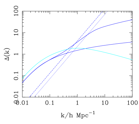
and $T(k,h,\Omega_{m})$ is the transfer function as given by Bardeen et al. (1986). The fiducial model we choose has parameters $(\delta_{H},h,\Omega_{m},b_{1},b_{2})=(5\times 10^{-5},0.65,0.3,0.002,1,0.5)$. For simplicity we assume spatial flatness. Figure 1 shows the spectrum used for subsequent calculations.

Figure 1: Fiducial matter power spectrum for a model galaxy redshift survey. The linear and nonlinear power in real-space (solid lines) are plotted alongside the angle averaged redshift power spectrum (light solid line) with small-scale damping included. The shot-noise per mode for both of the model surveys are also plotted (see table 1; 2dF (dot-dash) and SDSS (dotted).

5.2 Choosing bispectrum triangles

While our approach so far has been to retain as much information as possible, in practice it may not be possible to include all shapes of triangles in $k$-space due to CPU restrictions. It therefore makes sense to identify and study a subset of shapes that maximise the information content. We discuss this issue in more detail in Section 6. For simplicity we consider here only two distinct shapes: equilateral triangles and degenerate triangles. Degenerate triangles are constructed from two parallel wavevectors plus a third that is aligned anti-parallel with magnitude equal to the sum of the other two. A convenient subset of the degenerate category, and the configuration we shall consider in this analysis, has the magnitude of the two smaller wavevectors being equal. Constraints are made by inserting an appropriate dimensionless operator into equations (29) and (34). For equilateral triangles we use:

$$\Delta_{{\rm EQ}}=\int\!\frac{d^{3}\!k}{4\pi}\,\delta_{D}(k_{1}-k)\delta_{D}(k_{2}-k)\delta_{D}(k_{3}-k);$$ (43)

whereas for the subset of degenerate (DG) triangles one possible constraint is

$$\Delta_{{\rm DG}}=\frac{1}{4}\int\frac{d\mbox{\boldmath$k$}}{4\pi}\delta_{D}(k_{1}-k)\delta_{D}(k_{2}-k/2)\delta_{D}(k_{3}-k/2).$$ (44)

For the triangles of interest the bispectrum can be written

$$B(k)=\frac{12}{7}P^{2}(k)\;\;\;\;\;\;{\rm Equilateral}$$ (45)

$$B(k)=4P^{2}(k/2)-P(k/2)P(k)\;\;\;\;\;\;{\rm Degenerate}.$$ (46)

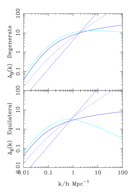
We plot the bispectra in Figure 2, where we have defined the function

$$\Delta^{2}_{B}(k)\equiv\frac{k^{3}\sqrt{B(k)}}{2\pi^{2}}$$ (47)

which is useful to compare with $\Delta^{2}(k)$.

For an ideal, finite survey, in the absence of shot-noise and redshift-space distortions, the nonlinear Fisher matrix for equilateral triangles can conveniently be reduced to

$${\cal F}_{ij} = \frac{V}{2}\!\int\!\!\frac{k^{2}dk}{2\pi^{2}}\Big{[}1+\Big{(}\frac{12}{7}\Big{)}^{2}\frac{\Delta^{2}(k)}{6}\Big{]}$$ (48)

$$\times\;[\partial_{i}\ln{\Delta^{2}(k)}][\partial_{j}\ln{\Delta^{2}(k)}].$$

Similar expressions for the parameter entropy and for the case of degenerate triangles can be found in appendix B.

The effect of including nonlinear terms is two-fold. Firstly we see that the bispectrum introduces a second, positive term into the Fisher matrix, driving the parameter uncertainty down. In addition, the nonlinear correction to the likelihood allows one to push the wave-range to higher $k$, again driving down the uncertainty.

Figure 2: Fiducial bispectra for the redshift survey model for equilateral triangles (bottom panel) and degenerate triangles (top panel). The real-space bispectra (heavy solid lines) are shown alongside the redshift-space bispectra (light solid lines) with small scale damping. The $P(k)/n$ noise term (dotted) and the $1/n^{2}$ noise term (dot-dashed) are also shown for a 2dF-type survey.

5.3 Poisson sampling of the density field

Assuming the measured galaxy population can be modelled as a random sampling of a smooth underlying field, the power- and bi-spectra transform according to

$$P(k)\!\!\! \rightarrow \!\!\!P(k)+\frac{1}{n},$$

$$B(\mbox{\boldmath$k$}_{1},\mbox{\boldmath$k$}_{2},\mbox{\boldmath$k$}_{3})\!\!\! \rightarrow \!\!\!B(\mbox{\boldmath$k$}_{1},\mbox{\boldmath$k$}_{2},\mbox{\boldmath$k$}_{3})$$ (49)

$$+\frac{1}{n}[P(k_{1})+P(k_{2})+P(k_{3})]+\frac{1}{n^{2}},$$

where $n$ is the mean number density of sources. If the noise varies across the survey, as is the case for flux-limited galaxy redshift surveys, this can be included in the models by the substitution $n=n(r)$ and $V\rightarrow\int\!d^{3}\!r$ in the Fisher and entropy estimates. For simplicity we work with the volume limited case and consider two models characterised by the number density, $n$, and survey volume, $V$, as given in Table 1. Noise levels for the surveys are plotted in Figures 1 and 2.

Survey	Mean Number	Effective
	Density ($n$)	Volume (V)
2dF	$3\times 10^{-3}$	$9\times 10^{7}$
SDSS	$10\times 10^{-3}$	$10\times 10^{7}$

Table 1: Parameters for two model redshift surveys considered in this paper.

5.4 Bias and redshift space distortions

The use of redshift coordinates as radial distance introduces a distortion in the observed density field;

$$\delta^{s}(\mbox{\boldmath$k$})=D(k\sigma\mu)(1+\beta\mu^{2})\delta(\mbox{\boldmath$k$}),$$ (50)

where the linear distortion modulates the density by a factor $(1+\beta\mu^{2})$ (Kaiser 1987) with $\beta=\Omega_{m}^{0.6}/b_{1}$ and $b_{1}$ the linear bias parameter. The small-scale pairwise velocity dispersion can be modeled by convolution of the density field with a random component along the line of sight (Peacock 1992, Peacock & Dodds 1994);

$$D(k\sigma\mu)=\frac{1}{\sqrt{1+k^{2}\sigma^{2}\mu^{2}/2}},$$ (51)

where $\mu=\mbox{\boldmath$\hat{r}$}.\mbox{\boldmath$\hat{k}$}$. Galaxy bias can be modeled by a local expansion of the density field (Fry and Gaztanaga 1993),

$$\delta_{g}=\sum_{m}\frac{b_{m}}{m!}\delta^{m}$$ (52)

where the coefficients $b_{m}$ are the bias parameters. The power spectrum for a biased, redshifted, and noisy galaxy survey is therefore

$$P^{s}_{g}(\mbox{\boldmath$k$})=b_{1}^{2}D^{2}(k\sigma\mu)(1+\beta\mu^{2})^{2}P(k)+\frac{1}{n}.$$ (53)

Note that we only consider the case of a deterministic bias, but this formalism can be easily generalised to include extra parameters for a stochastic biasing scheme (Pen 1998, Dekel & Lahav 1999).

For equilateral triangles the angles between the line of sight and the wavevectors of the bispectrum triangles are

$$\mu_{1} = \mu,$$

$$\mu_{2} = -\frac{1}{2}\mu+\frac{3}{2}\sqrt{1-\mu^{2}},$$

$$\mu_{3} = -\mu_{1}-\mu_{2},$$ (54)

where $\mu_{i}=\mbox{\boldmath$\hat{r}$}.\mbox{\boldmath$\hat{k}$}_{i}$. The corresponding redshifted bispectrum for equilateral triangles is (Hivon et al. 1995, Heavens et al. 1998, Verde et al. 1998, Scoccimarro et al. 1999)

$$B^{s}_{g}(\mbox{\boldmath$k$}) = D_{2}(k\sigma\mu)\Big{[}2b_{1}^{3}{\rm Ker}(k,\mu,\beta,b_{1})$$ (55)

$$+3b_{2}(1+\beta+3/16\beta^{2})\Big{]}P^{2}(k)$$

$$+\frac{1}{n}(D(k\mu_{1})(1+\beta\mu_{1}^{2})^{2}+{\rm cyc})P(k)+\frac{1}{n^{2}}$$

where $b_{2}$ is the second-order bias term and where kernel ${\rm Ker}(k,\mu,\beta,b_{1})$ is provided in Appendix B. Similar expressions for degenerate triangles can be obtained and are also given in the appendix. The redshifted power and bi-spectra are shown in Figures 1 and 2.

6 Results for a model galaxy redshift survey

6.1 Overview of parameter estimation

In this Section we apply the model outlined in Section 5 to estimate parameter uncertainties from two model galaxy redshift surveys, based on the 2dF and SDSS (see Table 1 for survey parameters). The parameters of the model are $(h,\delta_{H},\Omega_{m},b_{1},b_{2})$, with fiducial values given in Section 5.1. The model enters the analysis via the redshifted galaxy power spectrum, equation (53), and the bispectrum for equilateral triangles, equation (55), and degenerate triangles, equation (66). These are used to estimate the function $Q(\mbox{\boldmath$k$}_{1},\mbox{\boldmath$k$}_{2},\mbox{\boldmath$k$}_{3})$, given by equation (24), which is then used to calculate the nonlinear Fisher matrix, given by equations (29) and (19). The parameter entropy function is calculated from equations (32), (34), (35) and (36).

This section is laid out as follows. In Section 6.2 we present results for the marginalised parameter uncertainties for the two surveys, as a function of the truncation wavenumber for the Fourier integrals. Our basic result is that cosmological parameters may be estimated to accuracies of a few percent using redshift surveys independantly of other measurements. In Section 6.3 we show the correlation coefficients for all the parameters, again as a function of wavenumber, and illustrate that to second-order all of the degeneracies between parameters are lifted. We illustrate how parameter estimation is improved using a simplified two-parameter model in Section 6.4. We explore the relative information content of equilateral and degenerate triangles in Section 6.5. We begin with an estimation of the parameter uncertainties from the full model.

6.2 Nonlinear parameter estimation from redshift surveys

Figure 3: Marginalised error estimates on 5 parameters obtained from a Fisher analysis using the combined linear and nonlinear likelihood with equilateral and degenerate triangles. The results are shown for two sets of survey parameters resembling those of the 2dF (solid) and the SDSS (dot–dashed). Table 1 contains the survey parameters.

Marginal errors may be obtained from inversion of the Fisher matrix so that the the $1\sigma$ error on parameter $\theta_{i}$ is approximately given by

$$\Delta\theta_{i}=\sqrt{(\mbox{\boldmath${\cal F}$}^{-1})_{ii}},$$ (56)

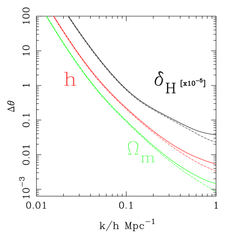
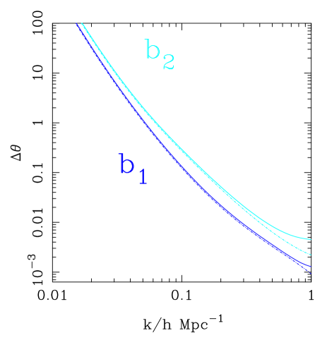
under the assumption that the likelihood distribution of parameters is roughly Gaussian. In Figure 3 we show the results of the Fisher analysis for the best attainable marginal uncertainties on the 5 independent parameters $\delta_{H},h,\Omega_{m},b_{1}$ and $b_{2}$ as a function of $k$. Here, and in subsequent figures, $k$ is the maximum mode, $k_{\rm max}$, in all integrations. A 5-D joint estimation of parameter uncertainties with the Fisher matrix is only possible for a nonlinear likelihood since to linear order the Fisher matrix is singular due to degeneracies between parameters.

We give the results for two different redshift surveys which we define by the volume of the survey, V, and the mean number density of sources, $n$. Formally this represents a volume-limited survey, but here we shall use effective values for a flux-limited sample. The volume and number density are chosen to resemble those of the 2dF redshift survey and the Sloan Digital Sky Survey. The relevant parameters are found in Table 1.

Interestingly, our results show that the accuracy of the parameter estimation is similar for the 2dF and the SDSS, for all of the parameters out to quite high k. The reason for this is that the effective volumes of the two surveys are similar (see Table 1), and the error scales like $1/\sqrt{V}$. Although the SDSS has a factor of $\approx 3$ higher density of galaxies than the 2dF, this does not become important until the models become noise dominated per mode. From Figures 1 and 2, we see that for both surveys, this is not until around $k=1\,h{\rm Mpc}^{-1}$, well below the scale where our parameter estimation is valid.

Figure 3 (LHS) shows the marginalised uncertainties on the parameters $\delta_{H}$, $h$ and $\Omega_{m}$. At $k=0.1\,h{\rm Mpc}^{-1}$, normally the limit of linear analysis (Heavens & Taylor 1995, Tadros et al. 1999, Hamilton, Tegmark & Padmanabhan 2000), the predicted uncertainties lie around the $\approx 30\%$ level for both $h$ and $\Omega_{m}$. Estimates for $\delta_{H}$, the horizon scale amplitude of matter perturbations, fare a little better at around $20\%$. Extending the analysis to $k=0.3\,h{\rm Mpc}^{-1}$, near the limit of second-order perturbation theory, we find the uncertainty falls by an order of magnitude to $\approx 2\%$ for all three parameters.

Figure 3 (RHS) also shows the marginalised parameter uncertainty for the bias parameters $b_{1}$ and $b_{2}$. For both surveys, truncated at $k=0.1\,h{\rm Mpc}^{-1}$, we find that $b_{2}$ is not detected at all, with $b_{1}$ detected at the $\approx 10\%$ level. However, if the analysis is pushed to $k=0.3\,h{\rm Mpc}^{-1}$ the error on $b_{1}$ drops to around a percent, while $b_{2}$ is now measured to around $5\%$ accuracy. While this looks encouraging for 2dF and the SDSS, we should caution that we have assumed a volume limited survey, with effective volume and noise levels chosen to mimic those of each survey. A more accurate assessment of the improved accuracy will require more detailed modeling and testing with N-body simulations, although the present study should provide a good indication of the measurement uncertainties.

6.3 Lifting all the parameter degeneracies in redshift surveys

As well as the marginal uncertainties it is interesting to consider the correlations between parameters. The information about such correlations lies in the off-diagonal components of the Fisher matrix. Defining the correlation coefficient for parameters $\theta_{i}$ and $\theta_{j}$ as

$$r_{ij}=\frac{({\cal F}^{-1})_{ij}}{\sqrt{({\cal F}^{-1})_{ii}({\cal F}^{-1})_{jj}}},$$ (57)

we can quantify the degree of correlation as a function of maximum wavenumber. The results are plotted in Figure 4 for all 10 of the correlation coefficients, $r_{ij}$, in the 5-dimensional parameter space considered above. The indices on the correlation coefficients are given in Table 2

Figure 4: Correlation coefficients for every pair of parameters in the 5-D marginalisation. The coefficients were calculated for the case of a 2dF-type survey and for a combined linear and nonlinear likelihood and both types of triangles. The key references Table 2 for the index of each parameter.

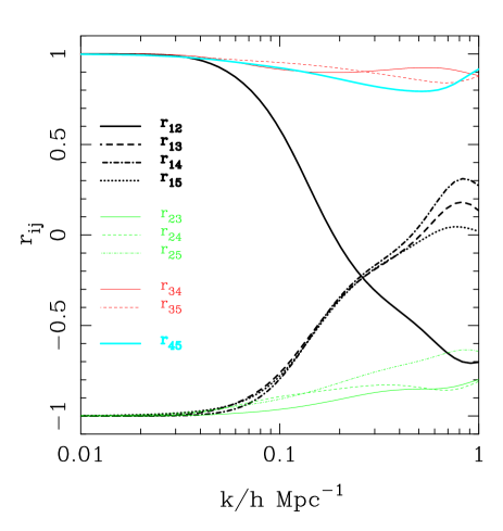
At low-$k$ the Fisher matrix is dominated by the linear contribution to the likelihood and subsequently all of the parameters remain perfectly correlated/anti-correlated ($r_{ij}=\pm 1$). The reason for this is that in the linear regime, one can only measure the three composite parameters, $\beta=\Omega_{m}^{0.6}/b_{1}$, from redshift-space distortions, $b_{1}\delta_{H}$ from the amplitude of linear galaxy clustering, and the spectral shape parameter, $\Gamma=\Omega_{m}h$, which determines the break scale in the matter power spectrum.

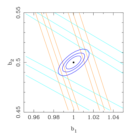
When the nonlinear terms begin to become important, at $k=0.04\,h{\rm Mpc}^{-1}$, the $r_{ij}$ deviate from $\pm 1$ indicating the decoupling of the parameters. The reason for this universal removal of degeneracies lies in the lifting of the degeneracy between the bias parameters, $b_{1}$ and $b_{2}$. With a single triangle shape, one can only measure the combination $b_{1}/(1+b_{2}/2J(\mbox{\boldmath$k$}_{1},\mbox{\boldmath$k$}_{2})b_{1})$ (Matarrese et al 1997). With a second triangle shape this constraint is lifted. Figure 5 illustrates this, where we have plotted the two degenerate likelihood contours for $b_{1}$ and $b_{2}$ for equilateral and degenerate triangles. The angle of intersection of these contours depends on the choice of triangles and is maximised by choosing very different shapes, motivating the choice of equilateral and degenerate triangles. With the bias degeneracy removed, the degeneracies in $\beta$, $\Gamma$ and $b_{1}\delta_{H}$ are all lifted.

While the parameters are no longer degenerate, many remain quite tightly correlated. The amplitude $\delta_{H}$ appears to become least correlated, becoming almost completely decoupled from the other 4 parameters. This is because to linear order it is only degenerate with $b_{1}$.

As $k$ gets larger, the $r_{ij}$ coefficients begin to show deviations from a steady decline; in some cases this results in them actually growing larger. This occurs because the correlations between parameters ultimately depend upon shape and size of the 1-$\sigma$ likelihood surface around its maximum. As this surface shrinks with increasing parameter information, it can change its shape, depending on the relative response to clustering information. This is what ultimately determines the correlation coefficient values.

Figure 5: Lifting the degeneracy of the bias parameters using a combination of different triangle shapes for the bispectrum. The contours denote the 1, 2 and 3$\sigma$ confidence regions for Gaussian entropy plus equilateral triangles and Gaussian plus degenerate triangles (faint lines) and for the combined effect (dark lines). The entropy has been marginalised over the amplitude $\delta_{H}$. Redshift distortions have been ignored and the noise and volume are similar to those of the 2dF

index	parameter
1	$\delta_{H}$
2	$h$
3	$\Omega_{m}$
4	$b_{1}$
5	$b_{2}$

Table 2: Cosmological parameters and their index for the correlation coefficient.

6.4 A two-parameter model

Figure 6: Parameter derivatives (top panel) and 1$\sigma$ error levels for the joint estimation of $b_{1}$ and $\Gamma$ in redshift space (bottom panel). The top panel shows the angle averaged derivative of the $Q$ function from equation (24) for equilateral triangles (solid lines) and degenerate triangles (dotted lines) taken with respect to each of the parameters. The bottom panel shows the joint errors on the parameters when using the Gaussian likelihood (solid line), when adding in the contribution from equilateral triangles (dashed line) and when adding in both equilateral and degenerate triangles (dotted line). The survey parameters closely resemble those of the 2dF, as listed in Table 1.

Figure 7: Entropy contours in the $b_{1}$ – $\Gamma$ plane. The contour levels correspond approximately to 1 and 2$\sigma$ confidence limits. From top left to bottom right the plots show: the Gaussian entropy; the Gaussian entropy (light lines) and the contribution from equilateral triangles (dark lines); the Gaussian entropy (light lines) and the contribution from degenerate triangles; and the Gaussian entropy (light lines) with the sum of the contribution from the Gaussian part plus equilateral and degenerate triangles (dark lines). For all plots $k_{max}$ was $0.2\,h{\rm Mpc}^{-1}$. The survey parameters closely resemble those of the 2dF.

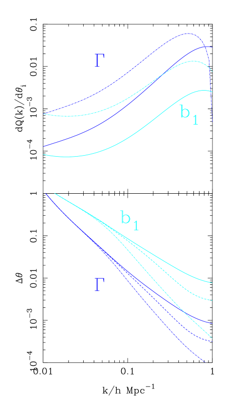
While the Fisher matrix results show the value of including nonlinear effects in parameter estimation, it is useful to examine in some more detail how nonlinearity increases parameter information. Rather than deal with all of the parameters, we shall restrict our analysis to two parameters. One is the linear bias factor, $b_{1}$, who’s measurement allows us to lift all the parameter degeneracies. The second is the parameter combination, $\Gamma=\Omega_{m}h$. The advantage of restricting our analysis to these two parameters is that their Fisher matrix in the linear regime is not singular, and can be compared directly with the nonlinear regime. We shall assume all other parameters are know.

In Figure 6 (top panel) we have plotted the derivatives of the nonlinear, angle-averaged, redshifted function $Q(\mbox{\boldmath$k$}_{1},\mbox{\boldmath$k$}_{2})$, given by equation (24) with respect to each of the parameters. This effectively shows the information content of the modes, with respect to each parameter. Dark lines show the derivative with respect to $\Gamma$, while lighter ones with respect to $b_{1}$. Solid lines are for equilateral triangles, while dotted lines show the contribution from degenerate triangles. Figure 6 shows that degenerate triangles have a higher derivative, indicating that they contain more information that equilateral ones. We shall return to this point in Section 6.5. The similarity of the shapes of the derivative also suggests that these parameters are strongly correlated.

In Figure 6 (bottom panel) we show the marginal $1\sigma$ uncertainties on $b_{1}$ and $\Gamma$ obtained from the Fisher analysis. It is immediately striking that inclusion of just a single triangle configuration has a significant effect on the errors. Even integrating out to relatively modest wavenumbers, $k\approx 0.2\,h{\rm Mpc}^{-1}$, there may be a 20 – 30 % reduction in the marginal uncertainty. This effect continues to grow as more modes are included. Using both triangle configurations has a much greater effect, reducing the errors by nearly an order of magnitude out at $k=0.3\,h{\rm Mpc}^{-1}$.

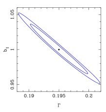
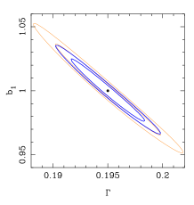
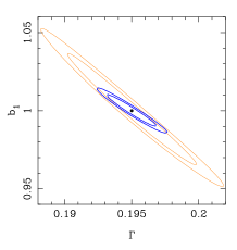
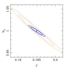
In Figure 7 we plot the entropy contours for a slice in the $b_{1}-\Gamma$ plane, assuming the other parameters are known. The top-left plot shows the Gaussian contribution to the parameter entropy, where the maximum wavenumber is $k_{\rm max}=0.2\,h{\rm Mpc}^{-1}$. The two parameters are highly correlated, and have uncertainties of $\Delta b_{1}\approx 0.05$ and $\Delta\Gamma\approx 0.005$. The top-right plot show the effect of adding nonlinear information from equilateral triangles; a $\approx 30\%$ improvement. By adding only degenerate triangles to the Gaussian term, in the bottom left figure, the uncertainty reduces more dramatically. Finally, in the bottom-right plot we show the combined effect of all of the terms.

Interestingly although the marginal errors are reduced, inclusion of the nonlinear terms does not, in this case, make the two parameters, $b_{1}$ and $\Gamma$, significantly less correlated, as suggested by the parameter derivatives in Figure 6. This can also be seen from the entropy contours in Figure 7 which are all rather elongated. The origin of this degeneracy is the effect both parameters have on the power spectrum. The linear bias factor, $b_{1}$, affects the amplitude of the power spectrum (ignoring its effects on redshift space distortions), while the shape parameter $\Gamma$ shifts the break scale in wavenumber. If the power spectrum were a power-law, these effects would be degenerate. But since there is a break, this degeneracy is broken on scales below the break scale. Adding nonlinear information, while reducing the absolute error, does not reduce this correlation.

6.5 The information content of triangles

It is apparent from Figures 5 and 6 that degenerate triangles seem to contain a great deal more information about cosmological parameters than equilaterals. As this result seems somewhat unintuitive, it is perhaps worth considering how the bispectrum triangles add information to the Fisher matrix.

The effect of different triangles can be partly understood from consideration of equation (29). For the non-Gaussian term, the Fisher matrix depends upon the derivatives of the function $Q(\mbox{\boldmath$k$}_{1},\mbox{\boldmath$k$}_{2})$ weighted by the product of $P(k_{1})P(k_{2})P(|\mbox{\boldmath$k$}_{1}+\mbox{\boldmath$k$}_{2}|)$. For equilateral triangles this factor is the cube of the power. However, for triangles where the magnitudes of the wavevectors are not equal there is a mixing of power from different scales. This implies is that information contained in a given triangle configuration is related to the shape of the power spectrum. Although the parameter derivatives of $Q(\mbox{\boldmath$k$}_{1},\mbox{\boldmath$k$}_{2})$ are larger for degenerate triangles, indicating a larger information content (see Figure 6), the power-weighting will ultimately determine which contributes the most information.

For monotonically rising $P(k)$, equilateral triangles are most significant because small scales (large $k$) contain most of the power. Conversely for power spectra that are decreasing functions of $k$, the maximum signal comes from large scales, hence for a given $k_{max}$, triangles that have a small side will give the most weight and provide the most information. In the CDM case the greatest power lies around the break scale, $k_{*}$. The result is therefore an admixture of the two competing effects; longwards of $k_{*}$ the spectrum rises and equilateral triangles contain the most information, shortwards and it is triangles that contain a short side that win out. In the limit this means that for CDM there is a “maximal” triangle for parameter estimation that is degenerate, in the manner discussed in Section (5.2), with sides $k_{*},k_{max},k_{max}-k_{*}$. In practise, estimating parameters from degenerate triangles may be more difficult, as there will be fewer independent low-$k$ modes within finite survey volume.

7 Conclusions

We have presented a method for including higher-order moments in the likelihood functions of cosmological fields in such a way that the parameter dependencies of the non-Gaussian terms may be used for estimating cosmological parameters. This non-Gaussian correction generalises likelihood analysis for application to fields that either contain intrinsic non-Gaussianity, or have become non-Gaussian due to nonlinear gravitational evolution. Such a generalisation is fundamentally important for cosmology since most of the interesting fields show non-Gaussian properties. Our method has the advantage that we attempt to deal with the probability distribution of the field explicitly, allowing the natural combination of linear and nonlinear regimes. In this respect our work differs significantly from existing techniques that separate out the nonlinear regime and apply a Gaussian PDF to the higher-order moments themselves (Matarrese et al. 1997, Verde et al. 1998, Scoccimarro et al. 1999, Scoccimarro et al. 2000).

We have presented a general formalism for calculating the non-Gaussian Fisher matrix and the shape of the likelihood around its maximum, the parameter entropy function. A central result of this paper has been to show that to lowest order, the dominant effect of adding nonlinearity, or more generally a non-Gaussianity, is to increase the the parameter information. This effect dominates over the degradation of parameter information due to the nonlinear evolution of the shape of the likelihood function.

Applying our analysis of nonlinearity to a simple model for a galaxy redshift survey, including the effects of shot-noise, redshift-space distortions and galaxy bias, we have found that nonlinear effects may be extremely useful for placing tight constraints upon cosmological parameters. Of crucial importance is the fact that even at second-order, degeneracies can be broken so that all of the cosmologically interesting parameters may be estimated independently. While going to higher-order may place tighter constraints on the nonlinear bias function through estimation of the series coefficients $b_{n}$, essentially redshift surveys offer up a great deal of their information without the need to turn to progressively more intricate perturbative calculations. In addition, this analysis suggests that galaxy redshift surveys can be used in isolation to determine cosmological parameters. This greatly enhances their power as parameter estimation can be compared from independent surveys, such as the CMB, cosmic velocity fields and weak lensing surveys and combined further to reduce uncertainties.

Our analysis relies upon a multivariate generalisation of the Edgeworth approximation for the probability distribution function. As such one should be careful to determine the range of applicability of second-order perturbation theory, and the series expansion of the likelihood function. It is well known from studies of 1-point distributions (Bernardeau & Kofman 1995, Juszkiewicz et al. 1995 Gaztañaga et al. 1999, Taylor & Watts 2000, Watts & Taylor 2000) that the Edgeworth PDF has limitations – displaying unphysical features when the variance or skewness becomes too high. However, these effects do not automatically render the Edgeworth a bad approximation. Comparison with N-body simulations in redshift-space (Watts & Taylor 2000) has shown that peak of the distribution remains a good fit even when the extremities begin to behave badly. Fortunately we have found that a good deal of information comes from the nonlinear terms at relatively low-$k$ and have shown that the degeneracies between parameters are broken even for modest values of wavenumber. This is good news from a computational point of view as well since the number of modes available for analysis grows like $k^{3}$. While this is beneficial in some respects, it can also lead to computational problems if the number of modes gets too high. In his case data compression methods may need to be incorporated (Taylor et al. 2000). In a forthcoming paper (Watts & Taylor, in preparation) we rigorously test our model on N-body simulations in order to accurately determine the limitations, and address the specific issues associated with application to real data sets.

References

Amendola L., 1996, MNRAS, 283, 983

Bardeen J.M., Bond J.R., Kaiser N., Szalay A.S., 1986, ApJ, 304, 15

Bernardeau F., Kofman L., 1995, ApJ, 443, 479

Bond J.R., Efstathiou G., Tegmark M., 1997, MNRAS, 291, L33

Bouchet F.R., Juszkeiwicz R., Colombi S., Pellat., 1992, ApJ, 394, L5

Coles P., Jones B., 1991, MNRAS, 248, 1

Colless M., 1998, In proc. 14th IAP meeting, Paris

Dekel A., Lahav O., 1999, ApJ, 520, 24

Folkes S., Ronen S., Price I., Lahav O., Colless M., Maddox S., Deeley K., Glazebrook K., Bland-Hawthorn J., Cannon R., Cole S., Collins C., Couch W., Driver S.P., Dalton G., Efstathiou G., Ellis R.S., Frenk C.S., Kaiser N., Lewis I., Lumsden S., Peacock J.A., Peterson B.A., Sutherland W., Taylor K., 1999, MNRAS, 308, 459

Fry J.N., 1994, Phys Rev Lett, 73, 215

Fry J.N., Gaztañaga E., 1993, ApJ, 413, 447

Gaztañaga E., Fosalba P., Elizalde E., 2000, ApJ, 539, 522

Goroff M., Grinstein B., Rey S., Wise M.B., 1986, ApJ, 311, 6

Gunn J.E., 1995, In proc. American Astronomical Society Meeting, 186, 4405

Hamilton A.J, Tegmark M., Padmanabhan N., 2000, MNRAS, 317, L23

Heavens A.F., Taylor A.N., 1995, MNRAS, 275, 483

Heavens A.F., Taylor A.N., 1997, MNRAS, 290, 456

Heavens A.F., Matarrese S., Verde L., 1998, MNRAS, 301, 797

Hivon E., Bouchet F.R., Colombi S., Juszkiewicz R., 1995, ApJ, 298, 643

Hu W., Tegmark M., 1999, ApJ, 514, L65

Jungman G., Kamionkowski M., Kosowsky A., Spergel D.N., 1996, Phys Rev D, 54, 1332

Juszkeiwicz R., Weinberg D.H., Amsterdamski P., Chodorowski M., Bouchet F., 1995, ApJ, 442, 39

Kaiser N., 1987, MNRAS, 227, 1

Kendal M.G., Stuart A., 1969, “The Advanced Theory of Statistics, Vol. 2”, Griffin, London

Ma C., Fry J.N., 2000, astro-ph/0003343

Maddox, S., 1998, In proc. ASP Conf. Ser. 146: The Young Universe: Galaxy Formation and Evolution at Intermediate and High Redshift

Matarrese S., Verde L., Heavens A.F., 1997, MNRAS, 290, 651

Peacock J.A., 1992, MNRAS, 258, 581

Peacock J.A., Dodds S.J., 1994, MNRAS, 267, 1020

Peacock J.A., Smith R.E., 2000, astro-ph/0005010

Peebles P.J., 1980, “Large-Scale Structure in the Universe”, Princeton University Press, Princeton

Pen U., 1998, ApJ, 504, 651

Rocha G., Magueijo J., Hobson M., Lasenby A., 2000, astro-ph/0008070

Scoccimarro R., Colombi S., Fry J.N., Frieman J.A., Hivon E., Melott A., 1998, ApJ, 496, 586

Scoccimarro R., Couchman H.M.P., Frieman J., 1999, ApJ, 517, 531

Scoccimarro R., Feldman H.A., Fry J.N., Frieman J., 2000 (astro-ph/0004087)

Seljak U., 2000, astro-ph/0001493

Tadros H., Ballinger W.E., Taylor A.N., Heavens A.F., Efstathiou G., Saunders W., Frenk C.S., Keeble O., McMahon R., Maddox S.J., Oliver S., Rowan-Robinson M., Sutherland W.J., White S.D.M., 1999, MNRAS, 305, 527

Taylor A.N., Watts P.I.R., 2000, MNRAS, 314, 92

Taylor A.N., Ballinger W.E., Heavens A.F.,Tadros H., 2000, astro-ph/0007048

Tegmark M., 1997, Phys Rev Lett, 79, 3806

Tegmark M., Taylor A.N., Heavens A.F., 1997, MNRAS, 480, 22

Verde L., Heavens A.F., Matarrese S., Moscardini L., 1998, MNRAS, 300, 747

Watts P.I.R., Taylor A.N., 2000, astro-ph/0006192

Appendix A

For completeness, we provide the general continuum form for the non-Gaussian perturbation term appearing in equation (7)

$$X = \int\!\prod_{i=1}^{4}d^{3}\!x_{i}\,D(\mbox{\boldmath$x$}_{1},\mbox{\boldmath$x$}_{2},\mbox{\boldmath$x$}_{3})\,C^{-1}(\mbox{\boldmath$x$}_{4},\mbox{\boldmath$x$}_{1})C^{-1}(\mbox{\boldmath$x$}_{2},\mbox{\boldmath$x$}_{3})\,\phi(\mbox{\boldmath$x$}_{4})+{\rm cyc}(231,312)$$ (58)

$$+ \int\!\prod_{i=1}^{6}d^{3}\!x_{i}\,D(\mbox{\boldmath$x$}_{1},\mbox{\boldmath$x$}_{2},\mbox{\boldmath$x$}_{3})\,C^{-1}(\mbox{\boldmath$x$}_{1},\mbox{\boldmath$x$}_{4})C^{-1}(\mbox{\boldmath$x$}_{2},\mbox{\boldmath$x$}_{5})C^{-1}(\mbox{\boldmath$x$}_{3},\mbox{\boldmath$x$}_{6})\,\phi(\mbox{\boldmath$x$}_{4})\phi(\mbox{\boldmath$x$}_{5})\phi(\mbox{\boldmath$x$}_{6})$$

where ${\rm cyc}$ means to permutate indices.

Appendix B

In the absence of noise and redshift distortions the nonlinear Fisher matrix and entropy can be written in a particularly pleasing form. The Fisher matrix for equilateral triangles reduces to

$${\cal F}_{ij}=\frac{V}{2}\!\int\!\!\frac{k^{2}dk}{2\pi^{2}}\Big{[}1+\Big{(}\frac{12}{7}\Big{)}^{2}\frac{\Delta^{2}(k)}{6}\Big{]}\,[\partial_{i}\ln{\Delta^{2}(k)}][\partial_{j}\ln{\Delta^{2}(k)}],$$ (59)

while the parameter entropy is given by

$$S=\frac{V}{2}\int\!\frac{k^{2}dk}{2\pi^{2}}\,\Big{\{}\ln{\Delta^{2}(k)}+\frac{\Delta^{\prime 2}(k)}{\Delta^{2}(k)}+\frac{1}{12}\Big{(}\frac{12}{7}\Big{)}^{2}\Delta^{\prime 2}(k)\Big{[}\Big{(}\frac{\Delta^{\prime 2}(k)}{\Delta^{2}(k)}\Big{)}^{2}-\frac{2\Delta^{\prime 2}(k)}{\Delta^{2}(k)}\Big{]}\Big{\}}.$$ (60)

For the case of degenerate triangles the Fisher matrix becomes

$${\cal F}_{ij} = \frac{V}{2}\!\int\!\!\frac{k^{2}dk}{2\pi^{2}}\Big{\{}\Big{[}1+\frac{8}{3}\frac{\left(\Delta^{2}(k/2)\right)^{2}}{\Delta^{2}(k)}\Big{]}\;[\partial_{i}\ln{\Delta^{2}(k)}][\partial_{j}\ln{\Delta^{2}(k)}]+\frac{1}{6}\Delta^{2}(k)\;[\partial_{i}\ln{\Delta^{2}(k/2)}][\partial_{j}\ln{\Delta^{2}(k/2)}]$$ (61)

$$\;\;\;-\frac{32}{3}\Delta^{2}(k/2)\;\Big{(}\partial_{[i}\ln{\Delta^{2}(k/2)}\;\partial_{j]}\ln{\Delta^{2}(k/2)}\Big{)}\Big{\}},$$

and the parameter entropy is

$$S = \frac{V}{2}\int\!\frac{k^{2}dk}{2\pi^{2}}\,\Big{\{}\ln{\Delta^{2}(k)}+\frac{\Delta^{\prime 2}(k)}{\Delta^{2}(k)}+\frac{1}{12}\Delta^{\prime 2}(k/2)\Big{[}\frac{\Delta^{\prime 2}(k/2)\Delta^{\prime 2}(k)}{[\Delta^{2}(k)]^{2}}-\frac{1}{2}\frac{\Delta^{\prime 2}(k/2)\Delta^{\prime 2}(k)}{\Delta^{2}(k/2)\Delta^{2}(k)}+\frac{1}{16}\frac{\Delta^{\prime 2}(k/2)\Delta^{\prime 2}(k)}{[\Delta^{2}(k/2)]^{2}}$$ (62)

$$\,\,-\frac{1}{2}\frac{\Delta^{\prime 2}(k/2)}{\Delta^{2}(k)}-\frac{1}{32}\frac{\Delta^{\prime 2}(k)}{\Delta^{2}(k/2)}+\frac{1}{8}\frac{\Delta^{\prime 2}(k/2)}{\Delta^{2}(k/2)}+\frac{1}{8}\frac{\Delta^{\prime 2}(k)}{\Delta^{2}(k)}\Big{]}\Big{\}}.$$

Appendix C: Redshifted Bispectrum

Here we present some of the formulae used to calculate the redshift space corrections for the bispectrum. The kernel from equation (55) for equilateral triangles is,

$${\rm Ker} = 3\,\Big{\{}\frac{2}{7}+\frac{1}{4}\beta(9/7+b_{1})+\frac{3}{112}\beta^{2}\Big{[}3-7b_{1}(2-b_{1})\Big{]}+\frac{1}{224}\beta^{3}\Big{[}\mu^{2}(3-4\mu^{2})^{2}+7b_{1}(1-b_{1}^{2})(9(1-\mu^{2})+8\mu^{4}(3-2\mu^{2}))\Big{]}$$ (63)

$$-\frac{1}{256}\beta^{4}(b_{1}-1)(27-144\mu^{2}+384\mu^{4}-256\mu^{6})\Big{\}}.$$

The nonlinear small scale damping factor is

$$D_{2}(k\sigma\mu) = \frac{1}{\sqrt{1+k^{2}\sigma^{2}\mu_{1}^{2}/2}}\frac{1}{\sqrt{1+k^{2}\sigma^{2}\mu_{2}^{2}/2}}\frac{1}{\sqrt{1+k^{2}\sigma^{2}\mu_{3}^{2}/2}}$$ (64)

$$= \frac{1}{\sqrt{1+3/4k^{2}\sigma^{2}+9/64k^{4}\sigma^{4}+k^{6}\sigma^{6}\mu^{2}(3-4\mu^{2})^{2}}}$$

The calculation in Section 5.4 can be repeated for degenerate triangles. In this case the angles between the line of sight and the wavevectors of the bispectrum triangles are

$$\mu_{1} = \mu,$$

$$\mu_{2} = -\mu$$

$$\mu_{3} = -\mu$$ (65)

The redshifted bispectrum is then given by

$$B^{s}_{g}(\mbox{\boldmath$k$}) = D_{2}(k,\mu)\Big{[}2b_{1}^{3}{\rm Ker}(k,\mu,\beta,b_{1})+b_{2}b_{1}^{2}(1+\beta\mu^{2})^{2}(2P(k)+P(k/2))\Big{]}P(k/2)$$ (66)

$$+\frac{1}{n}b_{1}^{2}D_{1}(k,\mu_{1})(1+\beta\mu_{1}^{2})^{2}P(k)+\frac{1}{n}b_{1}^{2}D_{1}(k,\mu_{2})(1+\beta\mu_{2}^{2})^{2}P(k/2)+\frac{1}{n}b_{1}^{2}D_{1}(k,\mu_{3})(1+\beta\mu_{3}^{2})^{2}P(k/2)+\frac{1}{n^{2}},$$

where in this case the kernel is

$${\rm Ker} = \frac{1}{2}\Big{[}4P(k/2)-P(k)\Big{]}+\frac{1}{2}\mu^{2}\Big{[}4(3+b_{1})P(k/2)-3P(k)\Big{]}\beta+\frac{1}{2}\mu^{4}\Big{[}(4b_{1}-4b_{1}^{2}-3)P(k)+2(5b_{1}+b_{1}^{2}+6)P(k/2)\Big{]}\beta^{2}$$ (67)

$$-\frac{1}{2}\mu^{6}\Big{[}(1-8b_{1}+8b_{1}^{2})P(k)-4(1+b_{1}^{2})P(k/2)\Big{]}\beta^{3}-b_{1}\mu^{8}\Big{[}(2-2b_{1})P(k)+(1+b_{1})P(k/2)\Big{]}\beta^{4},$$

and the damping term

$$D_{2}(k,\mu)=\frac{1}{\sqrt{(1+k^{2}\sigma^{2}\mu^{2}/8)(1+k^{2}\sigma^{2}\mu^{2}/2)}}$$ (68)