Acceleration of the Universe

Abstract

The cosmological model best capable of fitting current observational data features two separate epochs during which the Universe is accelerating. During the earliest stages of the Universe, such acceleration is known as cosmological inflation, believed to explain the global properties of the Universe and the origin of structure. Observations of the present state of the Universe strongly suggest that its density is currently dominated by dark energy with properties equivalent or similar to a cosmological constant. In these lecture notes, I provide an introductory account of both topics, including the possibility that the two epochs may share the same physical description, and give an overview of the current status.

1 Overview

The original cosmological models assumed a Universe that underwent deceleration during its entire evolution, corresponding to the slowing of the expansion through gravitational deceleration. As cosmology has developed, this assumption has been overturned at two separate epochs. It is now widely believed that the Universe underwent a phase of accelerated expansion, known as cosmological inflation, during some early stage of the Universe’s expansion. This hypothesis provides what is currently the best explanation for the observed structures in the Universe, especially cosmic microwave background anisotropies. In the present Universe evidence from many types of observation, most prominently the apparent magnitude–redshift relation of distant type Ia supernovae, suggests that the Universe is presently accelerating, which can be explained by the existence of a cosmological constant or an unusual form of matter sharing similar properties, often referred to as quintessence.

The purpose of this article is to provide an introductory review of these two topics, highlighting the ways in which the two phenomena may be a consequence of the same underlying physical mechanism — domination of the Universe by the energy density of a scalar field. It begins with an overview of inflation in the early Universe, with the focus very much directed towards inflation as a theory of the origin of structure. This is a particularly exciting time for proponents of this mechanism, as microwave anisotropy measurements from the BOOMERanG and MAXIMA experiments [1, 2] have given strong support to its basic predictions, opening the possibility of high-precision testing in the future. Later in the article, the current status of understanding of the present acceleration in the context of scalar field domination is discussed, and challenges and unsolved problems highlighted.

2 A Hot Big Bang reminder

2.1 Overview

To begin, I’ll give a quick review of the big bang cosmology. More detailed accounts can be found in any cosmology textbook. The main aim in this subsection is to set down the notation for the rest of the article.

The standard hot big bang theory, by which I mean the description of the Universe from a time of around one second onwards, is an extremely successful one, passing some crucial observational tests of which I’d highlight five.

• The expansion of the Universe.

• The existence and spectrum of the cosmic microwave background radiation.

• The abundances of light elements in the Universe (nucleosynthesis).

• That the predicted age of the Universe is comparable to direct age measurements of objects within the Universe.

• That given the irregularities seen in the microwave background by COBE, there exists a reasonable explanation for the development of structure in the Universe, through gravitational collapse.

In combination these are extremely compelling, and there is little doubt that the physical framework for describing the Universe from one second onwards is firmly in place, although the values of the various parameters required to specify the model in detail remain uncertain.

However, there is a series of questions which the standard big bang theory does not address. It does not predict the geometry of the Universe, except insofar as to indicate that a spatially-flat cosmology requires considerable fine-tuning of the initial conditions. It does not predict the relative abundances of different kinds of material — baryons, radiation, dark matter, etc — in the present Universe; these are assumed. And, most importantly of all, it does not offer an explanation for why the Universe was homogeneous to a high degree of accuracy at early times, but with sufficient irregularities within it to enable gravitational collapse to lead to structures such as galaxies and galaxy clusters. In order to address these questions, one must consider possible physical phenomena which might have taken place in the very early Universe, at epochs so early that the appropriate laws of physics are unknown. This raises the exciting possibility that an accurate determination of the properties of the present Universe might shed light on the physics of those early stages.

2.2 Equations of motion

The hot big bang theory is based on the cosmological principle, which states that the Universe should look the same to all observers. That tells us that the Universe must be homogeneous and isotropic, which in turn tells us which metric must be used to describe it. It is the Robertson–Walker metric

$$ds^{2}=-dt^{2}+a^{2}(t)\left[\frac{dr^{2}}{1-kr^{2}}+r^{2}\left(d\theta^{2}+\sin^{2}\theta\,d\phi^{2}\right)\right]\,.$$ (1)

Here $t$ is the time variable, and $r$–$\theta$–$\phi$ are (polar) coordinates. The constant $k$ measures the spatial curvature, with $k$ negative, zero and positive corresponding to open, flat and closed Universes respectively. If $k$ is zero or negative, then the range of $r$ is from zero to infinity and the Universe is infinite, while if $k$ is positive then $r$ goes from zero to $1/\sqrt{k}$. Many authors rescale the coordinates to make $k$ equal to $-1$, $0$ or $+1$. The quantity $a(t)$ is the scale-factor of the Universe, which measures its physical size. The form of $a(t)$ depends on the properties of the material within the Universe, as we’ll see.

If no external forces are acting, then a particle at rest at a given set of coordinates $(r,\theta,\phi)$ will remain there. Such coordinates are said to be comoving with the expansion. One swaps between physical (ie actual) and comoving distances via

$$\mbox{physical distance}=a(t)\times\mbox{comoving distance}\,.$$ (2)

The expansion of the Universe is governed by the properties of material within it. This can be specified by the energy density $\rho(t)$ and the pressure $p(t)$. These are often related by an equation of state, which gives $p$ as a function of $\rho$; the classic examples are

$$\mbox{Radiation:}\;\;p=\frac{\rho}{3}\quad;\quad\mbox{Non-relativistic matter:}\;\;p=0$$ (3)

In general though there need not be a simple equation of state; for example there may be more than one type of material, such as a combination of radiation and non-relativistic matter, and certain types of material, such as a scalar field, cannot be described by an equation of state at all.

The crucial equations describing the expansion of the Universe are

$$H^{2}=\frac{8\pi}{3m_{{\rm Pl}}^{2}}\,\rho-\frac{k}{a^{2}}+\frac{\Lambda}{3}\quad\quad$$ Friedmann equation (4)

$$\dot{\rho}+3H(\rho+p)=0\quad\quad\quad$$ Fluid equation (5)

where overdots are time derivatives and $H=\dot{a}/a$ is the Hubble parameter. In this equation $\Lambda$ is the cosmological constant; astronomers’ convention is to write this as a separate term, though physicists would typically be happier to consider it as part of the density $\rho$.

These can also be combined to give

$$\frac{\ddot{a}}{a}=-\frac{4\pi}{3m_{{\rm Pl}}^{2}}\left(\rho+3p\right)+\frac{\Lambda}{3}\quad\quad\mbox{Acceleration equation}$$ (6)

in which $k$ does not appear explicitly.

2.3 Standard cosmological solutions

When $k=\Lambda=0$ the Friedmann and fluid equations can readily be solved for the equations of state given earlier, leading to the classic cosmological solutions

$$\mbox{Matter Domination~{}~{}~{}~{}~{}~{}}p=0: \quad\rho\propto a^{-3}\quad\quad a(t)\propto t^{2/3}$$ (7)

$$\mbox{Radiation Domination~{}~{}~{}~{}~{}}p=\rho/3: \quad\rho\propto a^{-4}\quad\quad a(t)\propto t^{1/2}$$ (8)

In both cases the density falls as $t^{-2}$. When $k=0$ we have the freedom to rescale $a$ and it is normally chosen to be unity at the present, making physical and comoving scales coincide. The proportionality constants are then fixed by setting the density to be $\rho_{0}$ at time $t_{0}$, where here and throughout the subscript zero indicates present value.

A more intriguing solution appears for domination by the cosmological constant, namely

$$a(t)\propto\exp\left(Ht\right)\quad{\rm with}\quad H=\sqrt{\frac{\Lambda}{3}}\,.$$ (9)

This is equivalent to the solution for a fluid with equation of state $p_{\Lambda}=-\rho_{\Lambda}$. The fluid equation then gives $\dot{\rho}_{\Lambda}=0$ and hence $\rho_{\Lambda}\equiv\Lambda/8\pi G$.

More complicated solutions can also be found for mixtures of components. For example, if there is both matter and radiation the Friedmann equation can be solved using conformal time $\tau=\int dt/a$, while if there is matter and a non-zero curvature term the solution can be given either in parametric form using normal time $t$, or in closed form with conformal time.

2.4 Critical density and the density parameter

The critical density $\rho_{{\rm c}}$ is defined as that giving a spatially-flat geometry, $k=0$, in the absence of a cosmological constant. From the Friedmann equation, this implies

$$\rho_{{\rm c}}(t)=\frac{3m_{{\rm Pl}}^{2}H^{2}}{8\pi}\,.$$ (10)

Densities are often measured as fractions of $\rho_{{\rm c}}$:

$$\Omega(t)\equiv\frac{\rho}{\rho_{{\rm c}}}\,.$$ (11)

The quantity $\Omega$ is known as the density parameter, and can be applied to individual types of material as well as the total density.

A similar definition can be employed for the cosmological constant, giving

$$\Omega_{\Lambda}=\frac{\Lambda}{3H^{2}}\,,$$ (12)

and when both density and cosmological constant are present the condition for spatial flatness is $\Omega+\Omega_{\Lambda}=1$.

The present value of the Hubble parameter is still not that well known, and is parametrized as

$$H_{0}=100h\;{\rm km\,s}^{-1}\,{\rm Mpc}^{-1}=\frac{h}{3000}\,{\rm Mpc}^{-1}\,,$$ (13)

where $h$ is normally assumed to lie in the range $0.5\leq h\leq 0.8$. The present critical density is

$$\rho_{{\rm c}}(t_{0})=1.88\,h^{2}\times 10^{-29}\,{\rm g\,cm}^{-3}=2.77\,h^{-1}\times 10^{11}\,M_{\odot}/(h^{-1}{\rm Mpc})^{3}\,.$$ (14)

2.5 Characteristic scales and horizons

The big bang Universe has two characteristic scales

• The Hubble time (or length) $H^{-1}$.

• The curvature scale $a|k|^{-1/2}$.

The first of these gives the characteristic timescale of evolution of $a(t)$, and the second gives the distance up to which space can be taken as having a flat (Euclidean) geometry. As written above they are both physical scales; to obtain the corresponding comoving scale one should divide by $a(t)$. The ratio of these scales gives a measure of the total density; from the Friedmann equation we find

$$\sqrt{|\Omega+\Omega_{\Lambda}-1|}=\frac{H^{-1}}{a|k|^{-1/2}}\,.$$ (15)

A crucial property of the big bang Universe is that it possesses horizons; even light can only have travelled a finite distance since the start of the Universe $t_{*}$, given by

$$d_{{\rm H}}(t)=a(t)\int_{t_{*}}^{t}\frac{dt}{a(t)}\,.$$ (16)

For example, matter domination gives $d_{{\rm H}}(t)=3t=2H^{-1}$. In a big bang Universe, $d_{{\rm H}}(t_{0})$ is a good approximation to the distance to the surface of last scattering (the origin of the observed microwave background, at a time known as ‘decoupling’), since $t_{0}\gg t_{{\rm dec}}$.

2.6 Redshift and temperature

The redshift measures the expansion of the Universe via the stretching of light

$$1+z=\frac{a(t_{0})}{a(t_{{\rm emission}})}\,.$$ (17)

Redshift can be used to describe both time and distance. As a time, it simply refers to the time at which light would have to be emitted to have a present redshift $z$. As a distance, it refers to the present distance to an object from which light is received with a redshift $z$. Note that this distance is not necessarily the time multiplied by the speed of light, since the Universe is expanding as the light travels across it.

As the Universe expands, it cools according to the law

$$T\propto\frac{1}{a}\,.$$ (18)

The expansion preserves the thermal form, in the absence of interactions. In its earliest stages the Universe may have been arbitrarily hot and dense.

2.7 The history of the Universe

Presently the matter content of the Universe is dominated by non-relativistic matter, but because radiation reduces more quickly with the expansion, this implies that at earlier times the Universe was radiation dominated. During the radiation era temperature and time are related by

$$\frac{t}{1\,{\rm sec}}\simeq\left(\frac{10^{10}\,{\rm K}}{T}\right)^{2}\,.$$ (19)

The highest energies accessible to terrestrial experiment, generated in particle accelerators, correspond to a temperature of about $10^{15}\,{\rm K}$, which was attained when the Universe was about $10^{-10}\,{\rm sec}$ old. Before that, we have no direct evidence of the applicable physical laws and must use extrapolation based on current particle physics model building. After that time there is a fairly clear picture of how the Universe evolved to reach the present, with the key events being as follows:

• $10^{-4}$ seconds: Quarks condense to form protons and neutrons.

• 1 second: The Universe has cooled sufficiently that light nuclei are able to form, via a process known as nucleosynthesis.

• $10^{4}$ years: The radiation density drops to the level of the matter density, the epoch being known as matter–radiation equality. Subsequently the Universe is matter dominated.

• $10^{5}$ years: Decoupling of radiation from matter leads to the formation of the microwave background. This is more or less coincident with recombination, when the up-to-now free electrons combine with the nuclei to form atoms.

• $10^{10}$ years: The present.

A more precise time-line is given in many textbooks, e.g. Ref. [3].

3 The inflationary cosmology

That inflation can resolve the classic initial conditions of the Hot Big Bang model — the horizon, flatness and monopole problems — is well documented (see e.g. Ref. [4, 5]) and I will not repeat the discussion here. Instead I will proceed directly to the definition of inflation, and an explanation of the inflationary mechanism for the origin of structure.

3.1 The definition of inflation

Inflation is defined to be any epoch during which the Universe is accelerating, $\ddot{a}>0$, with respect to cosmic time. We can rewrite this in several different ways

$$\ddot{a}>0\quad\Longleftrightarrow\quad\frac{d(H^{-1}/a)}{dt}<0\quad\Longleftrightarrow\quad p<-\frac{\rho}{3}\,.$$ (20)

The second of these is the most useful, because it has the most direct geometrical interpretation. It says that the Hubble length, as measured in comoving coordinates, decreases during inflation. At any other time, the comoving Hubble length increases. This is the key property of inflation; although typically the expansion of the Universe is very rapid, the crucial characteristic scale of the Universe is actually becoming smaller, when measured relative to that expansion.

Quite a wide range of behaviours satisfy the inflationary condition. The classic one is de Sitter expansion, which arises when the Universe is dominated by a cosmological constant, which we saw earlier gives $a(t)\propto\exp\left(Ht\right)$. However realistic models of inflation usually deviate from this idealized situation, since inflation must come to an end to allow the successes of the standard Hot Big Bang to be reproduced after one second or so.

3.2 Scalar fields and their potentials

In order to obtain the required equation of state, a suitable material must come to dominate the density of the Universe. Such a material is a scalar field, which in particle physics is used to represent spin-zero particles and which we represent by $\phi$ throughout. It transforms as a scalar (that is, it is unchanged) under coordinate transformations. In a homogeneous Universe, the scalar field is a function of time alone.

At present no fundamental scalar field has been observed, but they proliferate in modern particle physics theories. In particular, supersymmetry associates a boson with every fermion (and vice versa), giving a multitude of scalar fields in any supersymmetric theory containing the Standard Model of particle physics.

The traditional starting point for particle physics models is the action, which is an integral of the Lagrange density over space and time and from which the equations of motion can be obtained. As an intermediate step, one might write down the energy–momentum tensor, which sits on the right-hand side of Einstein’s equations. Rather than begin there, I will take as my starting point expressions for the effective energy density and pressure of a homogeneous scalar field. These are obtained by comparison of the energy–momentum tensor of the scalar field with that of a perfect fluid, and are

$$\rho_{\phi} = \frac{1}{2}\dot{\phi}^{2}+V(\phi)\,$$ (21)

$$p_{\phi} = \frac{1}{2}\dot{\phi}^{2}-V(\phi)\,.$$ (22)

One can think of the first term in each as a kinetic energy, and the second as a potential energy. The potential energy $V(\phi)$ can be thought of as a form of ‘configurational’ or ‘binding’ energy; it measures how much internal energy is associated with a particular field value (including the mass–energy of the particle number density it represents). Normally, like all systems, scalar fields try to minimize this energy; however, a crucial ingredient which allows inflation is that scalar fields are not always very efficient at reaching this minimum energy state.

Note in passing that a scalar field cannot in general be described by an equation of state; there is no unique value of $p$ that can be associated with a given $\rho$ as the energy density can be divided between potential and kinetic energy in different ways. This is not particularly significant for early Universe inflation, but will be later when we discuss the present Universe.

3.3 Models of inflation

At present, understanding of fundamental physics is insufficient to give clear guidance as to how to build inflationary models. The present approach is therefore more phenomenological; we construct models of inflation, develop their predictions, and ultimately compare to observations in order to determine which properties are associated with successful models. So far, this approach has narrowed the range of possible models only modestly, and indeed theoretical ingenuity is creating new models more rapidly than observational improvements are ruling models out. Fortunately, it is projected that this state of affairs will soon change; upcoming observations of microwave anisotropies should have the capacity to exclude either all or nearly all of existing inflationary models.

A model of inflation consists of some number of scalar fields, plus a form for the potential of those fields. It may also require a specification of the means for ending inflation. Ordinarily, the working assumption is that only a single scalar field is dynamically important during inflation, possibly with a second static field providing an additional contribution to the energy density (see the later discussion of hybrid inflation). This single-field paradigm is the simplest assumption that can be made, and a useful initial goal is to investigate how well such a model can be constrained by data, and indeed whether or not the entire class of single-field models can be excluded. In the latter eventuality, the question will arise as to whether a more complicated inflationary model can keep the theory alive, or if one has to abandon the inflationary model for structure formation altogether. I will say a little on this later, but for the most part this article restricts its attention to the single-field case.

Assuming that a single field $\phi$ gives the complete dynamics, the model is given by a choice of $V(\phi)$. Until recently, this potential would have been required to vanish at the minimum, in order not to generate an unfeasibly large cosmological constant today (we see from the effective density and pressure of a scalar field that a non-vanishing potential at the minimum gives the equation of state $p=-\rho$ mimicking a cosmological constant). In such a case, inflation will necessarily terminate as the field approaches the minimum. However, this assumption need not be made if a second static field supplies a contribution to the energy density, which may mean that the global potential minimum occurs for a value of this field differing from the one it has during inflation. It may therefore be necessary to specify the value $\phi_{{\rm end}}$ at which inflation terminates, as well as the potential.

3.4 Equations of motion and solutions

Let us assume there is only a single dynamical scalar field, and that any extra contribution to the energy density from a second field is included in its potential $V(\phi)$. The equations for an expanding Universe containing a homogeneous scalar field are easily obtained by substituting Eqs. (21) and (22) into the Friedmann and fluid equations, giving

$$H^{2}=\frac{8\pi}{3m_{{\rm Pl}}^{2}}\left[V(\phi)+\frac{1}{2}\dot{\phi}^{2}\right]\,,$$ (23)

$$\ddot{\phi}+3H\dot{\phi}=-V^{\prime}(\phi)\,,\quad\quad$$ (24)

where prime indicates $d/d\phi$. Here I have ignored the curvature term $k$, as it will quickly become negligible once inflation starts. This is done for simplicity only; there is no obstacle to including that term if one wished.

Since

$$\ddot{a}>0\Longleftrightarrow p<-\frac{\rho}{3}\Longleftrightarrow\dot{\phi}^{2}<V(\phi)$$ (25)

we will have inflation whenever the potential energy dominates. This should be possible provided the potential is flat enough, as the scalar field would then be expected to roll slowly.

The standard strategy for solving these equations is the slow-roll approximation (SRA); this assumes that a term can be neglected in each of the equations of motion to leave the simpler set

$$H^{2} \;\simeq\; \frac{8\pi}{3m_{{\rm Pl}}^{2}}\,V$$ (26)

$$3H\dot{\phi} \;\simeq\; -V^{\prime}$$ (27)

If we define slow-roll parameters [6]

$$\epsilon(\phi)=\frac{m_{{\rm Pl}}^{2}}{16\pi}\,\left(\frac{V^{\prime}}{V}\right)^{2}\quad;\quad\eta(\phi)=\frac{m_{{\rm Pl}}^{2}}{8\pi}\,\frac{V^{\prime\prime}}{V}\,,$$ (28)

where the first measures the slope of the potential and the second the curvature, then necessary conditions for the slow-roll approximation to hold are

$$\epsilon\ll 1\quad;\quad|\eta|\ll 1\,.$$ (29)

Unfortunately, although these are necessary conditions for the slow-roll approximation to hold, they are not sufficient, since even if the potential is very flat it may be that the scalar field has a large velocity. A more elaborate version of the SRA exists, based on the Hamilton–Jacobi formulation of inflation [7], which is sufficient as well as necessary [8].

Note also that the SRA reduces the order of the system of equations by one, and so its general solution contains one less initial condition. It works only because one can prove [7, 8] that the solution to the full equations possesses an attractor property, eliminating the dependence on the extra parameter.

3.5 The relation between inflation and slow-roll

As it happens, the applicability of the slow-roll condition is closely connected to the condition for inflation to take place, and in many contexts the conditions can be regarded as equivalent. Let’s quickly see why.

The inflationary condition $\ddot{a}>0$ is satisfied for a much wider range of behaviours than just (quasi-)exponential expansion. A classic example is power-law inflation $a\propto t^{p}$ for $p>1$, which is an exact solution for an exponential potential

$$V(\phi)=V_{0}\exp\left[-\sqrt{\frac{16\pi}{p}}\,\frac{\phi}{m_{{\rm Pl}}}\right]\,.$$ (30)

We can rewrite the condition for inflation as

$$\frac{\ddot{a}}{a}=\dot{H}+H^{2}>0\quad\Longleftrightarrow\quad-\frac{\dot{H}}{H^{2}}<1\quad\stackrel{{\scriptstyle{\mbox{{\large$\sim$}}}}}{{\Longleftrightarrow}}\quad\frac{m_{{\rm Pl}}^{2}}{16\pi}\,\left(\frac{V^{\prime}}{V}\right)^{2}<1$$ (31)

where the last manipulation uses the slow-roll approximation. The final condition is just the slow-roll condition $\epsilon<1$, and hence

$$\mbox{Slow-roll}\Longrightarrow\mbox{Inflation}$$

Inflation will occur when the slow-roll conditions are satisfied (subject to some caveats on whether the ‘attractor’ behaviour has been attained [8]).

However, the converse is not strictly true, since we had to use the SRA in the derivation. However, in practice

Inflation $$\quad\stackrel{{\scriptstyle{\mbox{{\large$\sim$}}}}}{{\Longrightarrow}}\quad \epsilon<1$$

Prolonged inflation $$\quad\stackrel{{\scriptstyle{\mbox{{\large$\sim$}}}}}{{\Longrightarrow}}\quad \eta<1$$

The last condition arises because unless the curvature of the potential is small, the potential will not be flat for a wide enough range of $\phi$.

3.6 The amount of inflation

The amount of inflation is normally specified by the logarithm of the amount of expansion, the number of e-foldings $N$, given by

$$N\equiv\ln\frac{a(t_{{\rm end}})}{a(t_{{\rm initial}})}=\int_{t_{{\rm i}}}^{t_{{\rm e}}}\,H\,dt\simeq-\frac{8\pi}{m_{{\rm Pl}}^{2}}\int_{\phi_{{\rm i}}}^{\phi_{{\rm e}}}\,\frac{V}{V^{\prime}}\,d\phi\,,$$ (32)

where the final step uses the SRA. Notice that the amount of inflation between two scalar field values can be calculated without needing to solve the equations of motion, and also that it is unchanged if one multiplies $V(\phi)$ by a constant.

The minimum amount of inflation required to solve the flatness and horizon problems is about 70 $e$-foldings, i.e. an expansion by a factor of about $10^{30}$. Although this looks large, inflation is typically so rapid that most inflation models give much more.

3.7 A worked example: polynomial chaotic inflation

The simplest inflation model [9] arises when one chooses a polynomial potential, such as that for a massive but otherwise non-interacting field, $V(\phi)=m^{2}\phi^{2}/2$ where $m$ is the mass of the scalar field. With this potential, the slow-roll equations are

$$3H\dot{\phi}+m^{2}\phi=0\quad;\quad H^{2}=\frac{4\pi m^{2}\phi^{2}}{3m_{{\rm Pl}}^{2}}\,,$$ (33)

and the slow-roll parameters are

$$\epsilon=\eta=\frac{m_{{\rm Pl}}^{2}}{4\pi\phi^{2}}\,.$$ (34)

So inflation can proceed provided $|\phi|>m_{{\rm Pl}}/\sqrt{4\pi}$, i.e. as long as we are not too close to the minimum.

The slow-roll equations are readily solved to give

$$\phi(t) = \phi_{{\rm i}}-\frac{m\,m_{{\rm Pl}}}{\sqrt{12\pi}}\,t\,,$$ (35)

$$a(t) = a_{{\rm i}}\exp\left[\sqrt{\frac{4\pi}{3}}\,\frac{m}{m_{{\rm Pl}}}\,\left(\phi_{{\rm i}}t-\frac{m\,m_{{\rm Pl}}}{\sqrt{48\pi}}t^{2}\right)\right]\,,$$ (36)

(where $\phi=\phi_{{\rm i}}$ and $a=a_{{\rm i}}$ at $t=0$) and the total amount of inflation is

$$N_{{\rm tot}}=2\pi\,\frac{\phi_{{\rm i}}^{2}}{m_{{\rm Pl}}^{2}}-\frac{1}{2}\,.$$ (37)

This last equation can be obtained from the solution for $a$, but in fact is more easily obtained directly by integrating Eq. (32), for which one needn’t have bothered to solve the equations of motion.

In the older inflationary literature, it was typically assumed that in order for classical physics to be valid, we would require $V\ll m_{{\rm Pl}}^{4}$ but no other restriction would be necessary. In particular, considering scalar field theory in flat space-time, there is no particular meaning to the actual value of the scalar field (which for instance could be shifted by a constant). With those presumptions, we see that while sufficient inflation requires $|\phi|>m_{{\rm Pl}}$, one can readily get enough inflation provided $m$ is small enough, and indeed we will see later that $m$ is in fact required to be small from observational limits on the size of density perturbations produced, allowing far more than the minimum amount of inflation required to solve the various cosmological problems we originally set out to solve.

3.7.1 Multi-field theories

While much of early investigation of inflation featured potentials such as the massive field discussed above, such models are widely regarded by inflation model builders as unsatisfactory. The reason is that current thinking in particle physics is dominated by supersymmetry, implying that in a cosmological context we should be operating within the framework of supergravity. Once supergravity is brought into play, the numerical value of the scalar field acquires a well-defined meaning, and it is believed that its value must be less than the (reduced) Planck mass $m_{{\rm Pl}}/\sqrt{8\pi}$ if the potential is not to be vulnerable to large nonrenormalizable corrections, which typically will destroy slow-roll and anyway will render theoretical calculations unreliable. As we have just seen, one cannot obtain sufficient inflation (or indeed any at all) with the polynomial potential under this restriction, and this conclusion is fairly generic for models where there is only a single scalar field.

An attractive way of circumventing this problem is the hybrid inflation model [10], where a second field provides an additional energy density which dominates over that from the inflaton itself. A typical potential takes the form

$$V(\phi,\psi)=\frac{\lambda}{4}\left(\psi-M\right)^{4}+V(\phi)+\frac{1}{2}g^{2}\psi^{2}\phi^{2}\,,$$ (38)

where $g^{2}$ is the coupling constant governing the interaction between the two fields. This is shown in Fig. 1. For large inflaton values the coupling stabilizes $\psi$ at zero, where it contributes a potential energy $\lambda M^{4}/4$ but otherwise does not participate in the dynamics, so that the inflaton sees a potential

$$V_{{\rm eff}}(\phi)=V(\phi)+\frac{\lambda}{4}M^{4}\,.$$ (39)

The interesting case is where the constant term dominates, as it provides extra friction to the $\phi$ equation of motion which makes it roll much more slowly, enabling sufficient inflation without violating the condition $\phi\ll m_{{\rm Pl}}/\sqrt{8\pi}$. Inflation ends when the $\phi$ field drops below a critical value, destabilizing the $\psi$ field and allowing the system to rapidly evolve into its true minimum at $\phi=0$, $\psi=\pm M$.

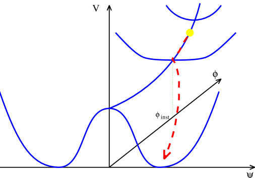
Figure 1: The potential for the hybrid inflation model. The field rolls down the channel at $\psi=0$ until it reaches the critical $\phi$ value, then falls off the side to the true minimum at $\phi=0$ and $\psi=\pm M$.

The original models [10] assumed that the inflaton potential $V(\phi)$ was just that of a massive field, but unfortunately this choice is vulnerable to large loop corrections which dominate over the mass term. However many other possible models have been derived within the hybrid framework; for an extensive discussion of this and other model-building issues see the review of Lyth and Riotto [11].

3.8 Reheating after inflation

During inflation, all matter except the scalar field (usually called the inflaton) is redshifted to extremely low densities. Reheating is the process whereby the inflaton’s energy density is converted back into conventional matter after inflation, re-entering the standard big bang theory. This may happen slowly due to decays of individual inflaton particles, or may begin explosively due to a coherent decay of the many-particle inflaton state. This latter possibility is known as preheating [12, 13] and may convert the bulk of the inflaton’s energy density. Preheating will however necessarily end before all the inflaton energy density is converted.

In the single field paradigm presently under discussion, it does not really matter how reheating takes place, in the sense that the details of the mechanism will not affect the predictions for large-scale structure. I therefore won’t discuss it further here, except to note that the situation can be considerably more complicated in multi-field theories. Then the details of reheating can be important for determining the magnitude of density perturbations in the Universe, and one also must consider possibilities such as that one or more of the fields need not decay at all, but may instead survive up to the present to act as dark matter or dark energy.

4 Density Perturbations and Gravitational Waves

By far the most important property of inflationary cosmology is that it produces perturbations, in the form of both density perturbations and gravitational waves. The density perturbations may be responsible for the formation and clustering of galaxies, as well as creating anisotropies in the microwave background radiation. The gravitational waves do not affect the formation of galaxies, but may contribute extra microwave anisotropies on the large angular scales sampled by the COBE satellite [14, 15]. An alternative terminology for the density perturbations is scalar perturbations and for the gravitational waves is tensor perturbations, the terminology referring to their transformation properties.

In this article I will focus on the nature of the predictions from the inflationary cosmology rather than detailed comparison with observations, which was the focus for a series of lectures at this Summer School by Pedro Viana [16].

4.1 Production during inflation

The ability of inflation to generate perturbations on large scales comes from the unusual behaviour of the Hubble length during inflation, namely that (by definition) the comoving Hubble length decreases. When we talk about large-scale structure, we are primarily interested in comoving scales, as to a first approximation everything is dragged along with the expansion. The qualitative behaviour of irregularities is governed by their scale in comparison to the characteristic scale of the Universe, the Hubble length.

In the big bang Universe the comoving Hubble length is always increasing, and so all scales are initially much larger than it, and hence unable to be affected by causal physics. Once they become smaller than the Hubble length, they remain so for all time. In the standard scenarios, COBE sees perturbations on large scales at a time when they were much bigger than the Hubble length, and hence no mechanism could have created them.

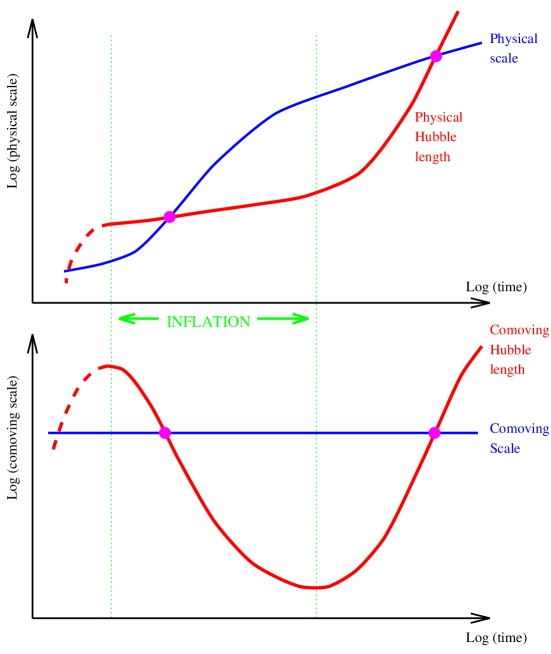
Figure 2: The behaviour of a given comoving scale relative to the Hubble length, both during and after inflation, shown using physical coordinates (upper panel) and comoving ones (lower panel).

Inflation reverses this behaviour, as seen in Figure 2. Now a given comoving scale has a more complicated history. Early on in inflation, the scale could be well inside the Hubble length, and hence causal physics can act, both to generate homogeneity to solve the horizon problem and to superimpose small perturbations. Some time before inflation ends, the scale crosses outside the Hubble radius (indicated by a circle in the lower panel of Figure 2) and causal physics becomes ineffective. Any perturbations generated become imprinted, or, in the usual terminology, ‘frozen in’. Long after inflation is over, the scales cross inside the Hubble radius again. Perturbations are created on a very wide range of scales, but the most readily observed ones range from about the size of the present Hubble radius (i.e. the size of the presently observable Universe) down to a few orders of magnitude less. On the scale of Figure 2, all interesting comoving scales lie extremely close together, and cross the Hubble radius during inflation very close together.

It’s all very well to realize that the dynamics of inflation permits perturbations to be generated without violating causality, but we need a specific mechanism. That mechanism is quantum fluctuations. Inflation is trying as hard as it can to make the Universe perfectly homogeneous, but it cannot defeat the Uncertainty Principle which ensures that there are always some irregularities left over. Through this limitation, it is possible for inflation to adequately solve the homogeneity problem and in addition leave enough irregularities behind to attempt to explain why the present Universe is not completely homogeneous.

The size of the irregularities depends on the energy scale at which inflation takes place. It is outside the scope of these lectures to describe in detail how this calculation is performed; the interested reader can find the full details in Ref. [3]. I will just quote the results, which we can go on to apply.

The formulae for the amplitude of density perturbations, which I’ll call $\delta_{{\rm H}}(k)$, and the gravitational waves, $A_{{\rm G}}(k)$, are 

$$\delta_{{\rm H}}(k) = \left.\sqrt{\frac{512\pi}{75}}\,\frac{V^{3/2}}{m_{{\rm Pl}}^{3}|V^{\prime}|}\right|_{k=aH}\,,$$ (40)

$$A_{{\rm G}}(k) = \left.\sqrt{\frac{32}{75}}\,\frac{V^{1/2}}{m_{{\rm Pl}}^{2}}\right|_{k=aH}\,.$$ (41)

Here $k$ is the comoving wavenumber; the perturbations are normally analyzed via a Fourier expansion into comoving modes. The power spectra $\delta_{{\rm H}}(k)$ and $A_{{\rm G}}(k)$ measure the typical size of perturbations on a scale $k$. The right-hand sides of the above equations are to be evaluated at the time when $k=aH$ during inflation, which for a given $k$ corresponds to some particular value of $\phi$. We see that the amplitude of perturbations depends on the properties of the inflaton potential at the time the scale crossed the Hubble radius during inflation. The relevant number of $e$-foldings from the end of inflation is given by [18]

$$N\simeq 62-\ln\frac{k}{a_{0}H_{0}}+\mbox{numerical correction}\,,$$ (42)

where ‘numerical correction’ is a typically smallish (order a few) number which depends on the energy scale of inflation, the duration of reheating and so on. Normally it is a perfectly fine approximation to say that the scales of interest to us crossed outside the Hubble radius 60 $e$-foldings before the end of inflation. Then the $e$-foldings formula

$$N\simeq-\frac{8\pi}{m_{{\rm Pl}}^{2}}\int_{\phi}^{\phi_{{\rm end}}}\,\frac{V}{V^{\prime}}\,d\phi\,,$$ (43)

tells us the value of $\phi$ to be substituted into Eqs. (40) and (41).

4.2 A worked example

The easiest way to see what is going on is to work through a specific example, the $m^{2}\phi^{2}/2$ potential which we already saw in Section 3.7. We’ll see that we don’t even have to solve the evolution equations to get our predictions.

1. Inflation ends when $\epsilon=1$, so $\phi_{{\rm end}}\simeq m_{{\rm Pl}}/\sqrt{4\pi}$.

2. We’re interested in 60 $e$-foldings before this, which from Eq. (37) gives $\phi_{60}\simeq 3m_{{\rm Pl}}$.

3. Substitute this in:

   $$\delta_{{\rm H}}\simeq 12\,\frac{m}{m_{{\rm Pl}}}\quad;\quad A_{{\rm G}}\simeq 1.4\,\frac{m}{m_{{\rm Pl}}}$$

4. Reproducing the COBE result requires [19] $\delta_{{\rm H}}\simeq 2\times 10^{-5}$ (provided $A_{{\rm G}}\ll\delta_{{\rm H}}$), so we need $m\simeq 10^{-6}m_{{\rm Pl}}$.

Because the required value of $m$ is so small, that means it is easy to get sufficient inflation to solve the cosmological problems if one only requires the classicality condition $V<m_{{\rm Pl}}^{4}$. Since that condition implies only that $\phi<m_{{\rm Pl}}^{2}/m\simeq 10^{6}m_{{\rm Pl}}$, and as $N_{{\rm tot}}\simeq 2\pi\phi^{2}/m_{{\rm Pl}}^{2}$, we can get up to about $10^{13}$ $e$-foldings in principle. This compares extremely favourably with the 70 or so actually required.

4.3 Observational consequences

Observations have moved on beyond us wanting to know the overall normalization of the potential. The interesting things are

1. The scale-dependence of the spectra.

2. The relative influence of the two spectra.

These can be neatly summarized using the slow-roll parameters $\epsilon$ and $\eta$ we defined earlier [6].

The standard approximation used to describe the spectra is the power-law approximation, where we take

$$\delta_{{\rm H}}^{2}(k)\propto k^{n-1}\quad;\quad A_{{\rm G}}^{2}(k)\propto k^{n_{{\rm G}}}\,,$$ (44)

where the spectral indices $n$ and $n_{{\rm G}}$ are given by

$$n-1=\frac{d\ln\delta_{{\rm H}}^{2}}{d\ln k}\quad;\quad n_{{\rm G}}=\frac{d\ln A_{{\rm G}}^{2}}{d\ln k}\,.$$ (45)

The power-law approximation is usually valid because only a limited range of scales are observable, with the range $1$ Mpc to $10^{4}$ Mpc corresponding to $\Delta\ln k\simeq 9$.

The crucial equation we need is that relating $\phi$ values to when a scale $k$ crosses the Hubble radius, which from Eq. (43) is

$$\frac{d\ln k}{d\phi}=\frac{8\pi}{m_{{\rm Pl}}^{2}}\,\frac{V}{V^{\prime}}\,.$$ (46)

(since within the slow-roll approximation $k\simeq\exp N$). Direct differentiation then yields [6]

$$n=1-6\epsilon+2\eta\quad;\quad n_{{\rm G}}=-2\epsilon\,,$$ (47)

where now $\epsilon$ and $\eta$ are to be evaluated on the appropriate part of the potential.

Finally, we need a measure of the relevant importance of density perturbations and gravitational waves. The natural place to look is the microwave background; a detailed calculation which I cannot reproduce here (see e.g. Ref. [18]) gives

$$R\equiv\frac{C_{\ell}^{{\rm GW}}}{C_{\ell}^{{\rm DP}}}\simeq\,4\pi\epsilon\,.$$ (48)

Here the $C_{\ell}$ are the contributions to the microwave multipoles, in the usual notation.

From these expressions we immediately see

• If and only if $\epsilon\ll 1$ and $|\eta|\ll 1$ do we get $n\simeq 1$ and $R\simeq 0$.

• Because the coefficient in Eq. (48) is so large, gravitational waves can have a significant effect even if $\epsilon$ is quite a bit smaller than one.

At present, a large number of inflationary models exist covering a large part of the $n$–$r$ parameter space. Observations are just beginning to narrow down the allowed region, and in the future satellite microwave anisotropy experiments such as MAP and Planck [20] should determine $n$ sufficiently accurately to exclude almost all models of inflation on that basis, and may be able to measure $r$ as well.

The principal observational challenge is to untangle the effects of the inflationary parameters ($\delta_{{\rm H}}(k_{0})$, $n$ and $r$) from all the other parameters required to specify a complete cosmological model, such as the Hubble constant, the density of each component of matter, and so on. The two sets of parameters cannot be studied separately; an attempt to match the observations must fit for both simultaneously. A typical set of parameters likely to be important in determining predictions for observations such as microwave anisotropies contains about ten different parameters, with some authors suggesting this list extends up to fifteen or more. It is a testament to the predicted accuracy of upcoming observations that considerable progress is expected in this direction over the next decade.

4.4 Testing the idea of inflation

An extremely useful sentence to bear in mind in considering how to test the inflationary paradigm is the following:

The simplest models of inflation predict a spatially-flat Universe containing gaussian distributed tensor and adiabatic scalar perturbations, which are in their growing mode with almost power-law spectra.

The underlined phrases indicate the characteristic predictions, while the emphasised word ‘simplest’ stresses that these predictions are not all generic. With the possible exception of the power-law form, the class of simplest models encompasses all the single-field models, plus many other models which prove to be dynamically equivalent to them

So far, all these characteristic predictions has been borne out, though the strength of the tests differs [16]. Only spatial flatness has really been confirmed at a convincing level, and even that only very recently [1, 2]. The others are promising hypotheses which are part of the currently-favoured view as to how structure arose.

The immediate goal is to test these hypotheses, and if they remain valid to use measured quantities such as $n$ and $r$ to establish which subset of the simplest models best fits the data. Our current aim, therefore, is to test the simplest models of inflation. If they are found wanting, then the way in which they fail will be indicative of whether it is worthwhile to study the wider range of inflation models, or if attention is best refocussed elsewhere. One should also stress that the aim is to test inflation as the sole origin of structure; one can consider admixtures of the inflationary perturbations with those of another source; this is fine if positive evidence is forthcoming but it will of course be impossible ever to exclude the possibility of an admixture at some level.

4.4.1 Growing mode perturbations

In general perturbations evolving on scales larger than the horizon have both growing and decaying modes, which on horizon entry become the baryonic oscillations. However because inflationary perturbations were laid down in the distant past, they evolve to become completely dominated by the growing mode by the time they enter the horizon. This leads to a fixed phase of oscillations for the baryons on a given scale; for example, at any given time (such as decoupling) there are particular scales on which the oscillations are at zero amplitude. On those scales the corresponding microwave anisotropies will be at their smallest. This contrasts with topological defect scenarios, where the modes are sourced after entering the horizon and in general have a mixture of the two perturbation modes, meaning that the phase of oscillation is not determined.

The growing mode prediction is perhaps the most important generic prediction of inflation, and one that cannot be avoided. It leads to characteristic predictions; the phase coherence of the oscillations that results is what leads to the oscillatory structure in the microwave anisotropy spectrum [21]. Such oscillations will arise whether the inflationary perturbations are gaussian or non-gaussian, and whether they are adiabatic or non-adiabatic. The prediction of an oscillatory structure in the microwave anisotropies is therefore a key testable prediction of inflation. That is not to say that the discovery of such would prove inflation, as other mechanisms may prove capable of also creating oscillations. But if the oscillations are not seen, the paradigm of inflation as the sole origin of structure will be excluded. The combined BOOMERanG and Maxima data are not quite sufficient for a definitive verdict, but tests of this prediction are imminent.

4.4.2 Gaussianity and adiabaticity

While gaussianity and adiabaticity are predictions of the simplest models, it is well advertised that there exist inflationary models which violate these hypotheses. Whether observations violating gaussianity or adiabaticity would exclude inflation depends on the type observed. For example, chi-squared distributed perturbations are relatively easy to generate from inflation, by ensuring that the leading contribution to perturbations is the square of a gaussian field. On the other hand, it would be pointless to try and find an inflation model if line discontinuities in the microwave sky were discovered.

4.4.3 Tensor and vector modes

Large-scale tensor modes are a generic prediction of inflation, but unfortunately the amplitude depends on the inflation model and there is no automatic implication that the tensor modes will have sufficient amplitude to be detectable by forseeable technology (indeed if anything theoretical prejudice suggests the opposite [22]). If tensor modes are discovered, for example by the Planck satellite, that will be exceedingly strong support for inflation. However tensor modes do not formally constitute a test of inflation, since their absence does not exclude the paradigm.

By contrast, the simplest inflationary models do not produce vector perturbations. If those are seen, then at the very least it will represent a considerable challenge to model-builders to find a way of accounting for them from within the inflationary paradigm.

4.4.4 Power-law spectra

It is currently fashionable to assume that the perturbation spectra, especially the scalars, take on a power-law form, just as it was fashionable pre-COBE to assume the Harrison–Zel’dovich form. Both these cases are approximations to the true situation, and as observations improve the power-law approximation may be found wanting just as the Harrison–Zel’dovich one was post-COBE. Staying within the single-field paradigm, unless prominent features are dialed into the inflationary potential, deviations from power-law behaviour are however predicted to be small, perhaps even by the standards to be imposed by the Planck satellite. Nevertheless, one should test for deviations when improved data come in [23, 24, 25].

5 Acceleration in the present Universe

5.1 Cosmological constant: exact or effective?

The discovery of strong evidence that the present Universe is accelerating is one of the most striking discoveries of recent cosmology. The results from Type Ia supernovae have been confirmed by two separate teams [26], and have subsequently stood up to detailed examination of the underlying mechanisms. The general conclusion has been further bolstered by support [1, 2] from the microwave background for the expectation that the Universe is spatially flat, which coupled with the observed low matter density gives independent demonstration of the need for a cosmological constant or similar.

These developments have confirmed the $\Lambda$CDM model as the standard cosmological model. It has a matter density around one third of the critical density, with the cosmological constant making up the remainder. It explains a range of phenomena concerning the observed content and dynamics of the Universe (including the age and the observed acceleration), and provides a model of structure formation which is not in serious disagreement with any existing observations. It is accepted almost universally amongst cosmologists that this model is currently the most observationally viable.

Despite that, the fraction of cosmologists willing to accept the $\Lambda$CDM model is significantly less, because of serious philosophical objections to the idea of a cosmological constant. First of all, there is absolutely no fundamental understanding of the cosmological constant. The standard interpretation is that it corresponds to the energy density of the vacuum state, but attempts to compute it typically result in answers so large as to be immediately excluded, leading to the suspicion that some as-yet-unknown physical mechanism sets it precisely to zero. This is known as the cosmological constant problem. Secondly, that the cosmological constant has just come to dominate at the present epoch marks out this time as a special point in the Universe’s history; at a redshift of a few it was completely negligible, and within a Hubble time it will be completely dominant. As the historical theme of cosmology has been to avoid placing ourselves at preferred locations both spatially and temporally, this situation causes great unease and has become known as the coincidence problem.

The observed value of the cosmological constant is that it is close to the critical density, which in particle physics units gives

$$\Lambda\simeq(0.003\,{\rm eV})^{4}\simeq 10^{-120}\,m_{{\rm Pl}}^{4}\,.$$ (49)

The naïvest fundamental physics estimates of the vacuum energy assume no suppression of contributions to the vacuum energy all the way to the Planck scale, and thus yield $\Lambda\simeq m_{{\rm Pl}}^{4}$. Reasonable arguments can bring this down to the scale of supersymmetry, $\Lambda=m_{{\rm susy}}^{4}\simeq 10^{-64}\,m_{{\rm Pl}}^{4}$, by presuming that at energies where supersymmetry is restored the bosonic and fermionic contributions to the cosmological constant cancel exactly. The vast discrepancy between expectation and reality puts us in an awkward situation; either we have to find an argument for a dimensionless prefactor to that estimate making up the remaining factor of $10^{-56}$, or we might conclude that there must be some fundamental principle setting it to zero leaving us to look elsewhere.

For an early Universe cosmologist, the temptation is irresistible to try and employ the same physical mechanisms in the present Universe as we did for inflation in the early Universe. Both correspond to an acceleration of Universe, and both could be the consequence of domination of the Universe’s energy density by the potential energy of a scalar field. Because we know, for example from nucleosynthesis, that there must have been a longer deceleration phase in between these two epochs, with some notable exceptions [27] the standard assumption is that different scalar fields are responsible for the two epochs, but that the physical mechanism is analogous. Describing the cosmological constant as an effective one via a scalar field has become known as quintessence, though that is a recent term to describe an idea with quite a long history [28, 29].

As far as modelling is concerned, there are some differences between the early Universe and today. In the early Universe, we know that inflation has to come to an end, and arranging that this happens satisfactorily is a significant constraint on model building. By contrast, we have no idea whether the present acceleration will end in the future. Secondly, in the present Universe we are interested in the earliest stages of the acceleration, and indeed the way in which the Universe entered the accelerating phase, and so we cannot neglect the effect of the non-scalar field matter as is common in early Universe inflation studies.

Broadly speaking, one can recognize three different possibilities. One is that in our Universe the scalar field is in the true minimum of its potential, whose value happens to be non-zero. Phenomenologically this is no different from a true cosmological constant. Secondly, we might live in a metastable false vacuum state, destined at some future epoch to tunnel into the true vacuum. Such tunnelling would almost certainly have drastic consequences for the material world, but we can be somewhat reassured by the fact that the decay time is at least a Hubble time. The false vacuum in this case also mimics a cosmological constant. Neither of these scenarios give us the possibility of addressing the coincidence problem, so mostly attention has been focussed on the third possibility, that the scalar field is slowly rolling in its potential akin to the chaotic inflation models. In this situation, the effective cosmological constant is in fact not constant at all but rather is slowly varying, and as such observations can seek to distinguish it from a pure cosmological constant.

5.2 Scaling solutions and trackers

One reason for having optimism that quintessence can at least address the coincidence problem comes from an interesting class of solutions known as scaling solutions or trackers. These arise because the scalar field does not have a unique equation of state $p\equiv p(\rho)$. Although we can usefully define an effective equation of state

$$w_{\phi}\equiv\frac{p_{\phi}}{\rho_{\phi}}=\frac{\dot{\phi}/2-V(\phi)}{\dot{\phi}/2+V(\phi)}\,,$$ (50)

in which terminology cosmological constant behaviour corresponds to $w=-1$, the scalar field velocity depends on the Hubble expansion, which in turn depends not only on the scalar field itself but on the properties of any other matter that happens to be around. That is to say, the scalar field responds to the presence of other matter.

A particularly interesting case is the exponential potential

$$V(\phi)=V_{0}\exp\left[-\sqrt{\frac{8\pi}{m_{{\rm Pl}}^{2}}}\,\lambda\phi\right]\,,$$ (51)

which we already saw in the early Universe context as Eq. (30). If there is only a scalar field present, this model has inflationary solutions $a\propto t^{2/\lambda^{2}}$ for $\lambda^{2}<2$, and non-inflationary power-law solutions otherwise. However, if we add conventional matter with equation of state $p=w\rho$, a new class of solutions can arise, which turn out to be attractors whenever they exist [28, 29, 30]. These solutions take the form of scaling solutions, where the scalar field energy density (indeed both its potential and kinetic energy density separately) exhibit the same scaling with redshift as the conventional matter. That is to say, the scalar field mimics whatever happens to be the dominant matter in the Universe. So, for example, in a matter-dominated Universe, we would find $\rho_{\phi}\propto 1/a^{3}$. If the matter era were preceded by a radiation era, at that time the scalar field would redshift as $1/a^{4}$, and it would make a smooth transition between these behaviours at equality. The ratio of densities is decided only by the fundamental parameters $\lambda$ and $w$. So, at any epoch one expects the scalar field energy density to be comparable to the conventional matter.

Unfortunately this is not good enough. We don’t want the scalar field to be behaving like matter at the present, since it is supposed to be driving an acceleration, and we need it to be negligible in the fairly recent past. This requires us to consider alternatives to the exponential potential, a common example being the inverse power-law potential [28]

$$V(\phi)=\lambda m_{{\rm Pl}}^{4}\left(\frac{\phi}{m_{{\rm Pl}}}\right)^{\alpha}\,,$$ (52)

where $\alpha<0$. In fact, Liddle and Scherrer [31] gave a complete classification of Einstein gravity models with scaling solutions, defined as models where the scalar field potential and kinetic energies stay in fixed proportion. The exponential potential is a particular case of that, but in general the scaling of the components of the scalar field energy density need not be the same as the scaling of the conventional matter, and indeed the inverse power-law potential is an example of that; if the conventional matter is scaling as $1/a^{m}$ where $m=3(1+w)$, there is an attractor solution in which the scalar field densities will scale as

$$\rho_{{\rm kinetic}}\propto\rho_{{\rm potential}}\propto\frac{1}{a^{n}}\quad;\quad n=\frac{\alpha}{\alpha-2}\,m\,.$$ (53)

With negative $\alpha$, the scalar field energy density is redshifting more slowly and eventually overcomes the conventional matter, at which point the Universe starts to accelerate.

This type of scenario can give a model capable of explaining the observational data, though it turns out that quite a shallow power-law is required in order to get the field to be behaving sufficiently like a cosmological constant (current limits require $w_{\phi}<-0.6$ at the present epoch, where $\Omega_{\phi}\simeq 0.7$ [32]). Also, the epoch at which the field takes over and drives an acceleration is still more or less being put in by hand; it turns out that the acceleration takes over when $\phi\simeq m_{{\rm Pl}}$, and so $\lambda\simeq 10^{-120}$ is required to ensure this epoch is delayed until the present.

Various other forms of the potential have been experimented with, and many possibilities are known to give viable evolution histories [33]. While such models do give a framework for interpretting the type Ia supernova results, in many cases with the possibility ultimately of being distinguished from a pure cosmological constant, I believe it is fair to say that so far no very convincing resolution of either the cosmological constant problem or the coincidence problem has yet appeared. However, quintessence is currently the only approach which has any prospect of addressing these issues.

5.3 Challenges for quintessence

At the moment quintessence is viable but lacks clear motivation, and greater observational input is needed before it will be possible to decide if it is really along the right track. The supernova measurements so far are not capable of giving very serious constraints, but this will hopefully change in the near future, both by observations extending to higher redshift and by improved measurements and statistics both at redshifts approaching one, where most of the current data is, and in the local calibrating sample. One exciting prospect is a dedicated satellite project which is currently under consideration, which may allow current systematic errors to be addressed as well as delivering a vastly larger data set. Concerning non-supernova observations, improved constraints on parameters such as $\Omega_{0}$, for instance from structure formation, would be welcome and will inform studies of quintessence. It may even eventually prove possible to spot the time evolution of quintessence by its effect on the microwave background through the integrated Sachs–Wolfe effect.

The two outstanding issues are the magnitude of the cosmological constant and why it should come to dominate at the present epoch. For a pure cosmological constant these are one and the same, and at present no lines of attack offer themselves. For quintessence, one question is whether there is an energy scale in fundamental physics comparable to the cosmological constant energy density (numerologists might consider for instance the similarity between the cosmological constant energy density and the measured neutrino mass-squared difference).

As to the coincidence problem, a very attractive, though as yet unrealized, notion is triggered quintessence, where the scalar field comes to dominate because a change in its behaviour is triggered by some other event. The obvious such recent event is matter–radiation equality, which occurred at a redshift of a few thousand. The ideal scenario would have perfect tracking during radiation domination, but a different behaviour during the matter era leading to domination after a suitable delay. At first sight, it seems that it might be possible to arrange this by coupling the quintessence field to the Ricci scalar, which vanishes in a perfect radiation dominated universe but is non-zero during matter domination. Several such models have been studied [34], but unfortunately triggered quintessence has yet to be realised in a natural way and it is looking increasingly doubtful that this line of attack will prove fruitful.

6 Summary

The aim of this article has been to recount how we go about describing two epochs of the Universe’s evolution during which it may have experienced accelerated expansion, and to highlight possible similarities in those descriptions. It is an appealing possibility that the same underlying mechanism may be responsible in each case.

Concerning the early Universe, I have introduced some of the facets of inflation in a fairly simple manner. If you are interested in going beyond this, a detailed account of all aspects of the inflationary cosmology can be found in Ref. [3]. Additional material on particle physics and model building aspects of inflation can be found in Ref. [11].

At present, inflation is the most promising candidate theory for the origin of perturbations in the Universe. Different inflation models lead to discernibly different predictions for these perturbations, and hence high-accuracy measurements are able to distinguish between models, excluding either all or the vast majority of them. Since its inception, the inflationary cosmology has been a gallery of different models, and the gallery has continually needed extension after extension to house new acquisitions. In all the time up to the present, very few models have been discarded. However, the near future holds great promise to finally begin to throw out inferior models, and, if the inflationary cosmology survives as our model for the origin of structure, we can hope to be left with only a narrow range of models to choose between.

Concerning the present Universe, quintessence is an interesting idea which is still in its early days as far as observations are concerned. It provides a framework in which to study the possibility of an accelerating Universe at present, but so far it has not completely lived up to its initial promise as a way of challenging problems such as the coincidence problem. There appears to be plentiful scope for further investigations of possible quintessence scenarios to try and remedy this shortcoming, especially in anticipation of improved observations in years to come. At present, there is little in the way of rivals to quintessence in terms of allowing a quantitative description of the recent evolution of the Universe.

References

- [1] P. de Bernardis et al., Nature 404, 955 (2000); A. E. Lange et al., astro-ph/0005004.
- [2] S. Hanany et al., astro-ph/0005123; A. Jaffe et al., astro-ph/0007333.
- [3] A. R. Liddle and D. H. Lyth, Cosmological Inflation and Large-Scale Structure, Cambridge University Press, Cambridge, 2000.
- [4] A. H. Guth, Phys. Rev. 23, 347 (1981).
- [5] E. W. Kolb and M. S. Turner, The Early Universe, Addison-Wesley, Redwood City, California (1990) [updated paperback edition 1994].
- [6] A. R. Liddle and D. H. Lyth, Phys. Lett. B 291, 391 (1992).
- [7] D. S. Salopek and J. R. Bond, Phys. Rev. D 42, 3936 (1990).
- [8] A. R. Liddle, P. Parsons and J. D. Barrow, Phys. Rev. D 50, 7222 (1994).
- [9] A. D. Linde, Particle Physics and Inflationary Cosmology, Harwood Academic, Chur, Switzerland (1990).
- [10] A. D. Linde, Phys. Lett. B 259, 38 (1991), Phys. Rev. D 49, 748 (1994); E. J. Copeland, A. R. Liddle, D. H. Lyth, E. D. Stewart and D. Wands, Phys. Rev. D 49, 6410 (1994).
- [11] D. H. Lyth and A. Riotto, Phys. Rep. 314, 1 (1998).
- [12] L. Kofman, A. D. Linde and A. A. Starobinsky, Phys. Rev. Lett. 73, 3195 (1994); A. D. Linde, astro-ph/9601004; L. Kofman, astro-ph/9605155.
- [13] Y. Shtanov, J. Traschen and R. Brandenberger, Phys. Rev. D 51, 5438 (1995); D. Boyanovsky, M. D’Attanasio, H. de Vega, R. Holman, D.-S. Lee and A. Singh, Phys. Rev. D 52, 6805 (1995).
- [14] G. F. Smoot et al., Astrophys. J. 396, L1 (1992).
- [15] C. L. Bennett et al., Astrophys. J. 464, L1 (1996).
- [16] P. T. P. Viana, in these proceedings, astro-ph/0009492.
- [17] J. E. Lidsey, A. R. Liddle, E. W. Kolb, E. J. Copeland, T. Barriero and M. Abney, Rev. Mod. Phys 69, 373 (1997).
- [18] A. R. Liddle and D. H. Lyth, Phys. Rep 231, 1 (1993).
- [19] E. F. Bunn and M. White, Astrophys. J. 480, 6 (1997); E. F. Bunn, A. R. Liddle and M. White, Phys. Rev. D 54, 5917R (1996).
- [20] map home page at http://map.gsfc.nasa.gov/; Planck home page at http://astro.estec.esa.nl/Planck/.
- [21] A. Albrecht, D. Coulson, P. Ferreira and J. Magueijo, Phys. Rev. Lett. 76, 1413 (1996); W. Hu and M. White, Phys. Rev. Lett. 77, 1687 (1996).
- [22] D. H. Lyth, Phys. Rev. Lett. 78, 1861 (1997).
- [23] E. J. Copeland, E. W. Kolb, A. R. Liddle and J. E. Lidsey, Phys. Rev. D 48, 2529 (1993), 49, 1840 (1994).
- [24] A. Kosowsky and M. Turner, Phys. Rev. D 52, 1739 (1995).
- [25] E. J. Copeland, I. J. Grivell and A. R. Liddle, Mon. Not. R. Astron. Soc. 298, 1233 (1998).
- [26] S. Perlmutter et al., Nature 391, 51 (1998); B. P. Schmidt et al., Astrophys. J. 507, 46 (1998).
- [27] P. J. E. Peebles and A. Vilenkin, Phys. Rev. D 59, 063505 (1999); E. J. Copeland, A. R. Liddle and J. E. Lidsey, astro-ph/0006421.
- [28] B. Ratra and P. J. E. Peebles, Phys. Rev. D 37, 3406 (1988).
- [29] C. Wetterich, Nucl. Phys. B302, 668 (1988).
- [30] E. J. Copeland, A. R. Liddle and D. Wands, Ann. Rev. NY Acad. Sci. 688, 647 (1993), Phys. Rev. D 57, 4686 (1998).
- [31] A. R. Liddle and R. J. Scherrer, Phys. Rev. D 59, 023509 (1999).
- [32] P. Brax and J. Martin, Phys. Lett. B 468, 40 (1999); L. Wang, R. R. Caldwell, J. P. Ostriker and P. J. Steinhardt, Astrophys. J. 530, 17 (2000); G. Eftathiou, Mon. Not. Roy. Astr. Soc. 310, 842 (2000).
- [33] G. Huey, L. Wang, R. Dave, R. R. Caldwell and P. J. Steinhardt, Phys. Rev. D 59, 063005 (1999); I. Zlatev, L. Wang and P. J. Steinhardt, Phys. Rev. Lett. 82, 896 (1999); A. Albrecht and C. Skordis, Phys. Rev. Lett. 84, 2076 (2000); S. Dodelson, M. Kaplinghat and E. Stewart, astro-ph/0002360.
- [34] J.-P. Uzan, Phys. Rev. D 59, 123510 (1999); L. Amendola, Phys. Rev. D 60, 043501 (1999); F. Perrotta, C. Baccigalupi and S. Matarrese, Phys. Rev. D 61, 023507 (2000).