Reverberation Measurements of Quasars and the Size-Mass-Luminosity Relations in Active Galactic Nuclei
Abstract
A 7.5 years spectrophotometric monitoring program of 28 Palomar-Green quasars to determine the size of their broad emission line region (BLR) is reviewed. We find both the continuum and the emission line fluxes of all quasars to vary during this period. Seventeen objects has adequate sampling for reverberation mapping and in all of them we find the Balmer line variations to lag those of the continuum by 100 days. This study increases the available luminosity range for studying the size–mass–luminosity relations in active galactic nuclei (AGNs) by two orders of magnitude and doubles the number of objects suitable for such studies. Combining our results with data available for Seyfert 1 galaxies, we find the BLR size to scale with the rest-frame 5100 Å luminosity as . This result is different from previous studies, and suggests that the effective ionization parameter in AGNs may be a decreasing function of luminosity. We are also able to constrain, subject to the assumption that gravity dominates the motions of the BLR gas, the scaling relation between the mass of the central black hole and the AGN’s luminosity. We find that the central mass scales with the 5100 Å luminosity as .
A program to monitor 11 high-luminosity quasars is presented here for the first time. Preliminary results from this program indicate continuum variation of order of 0.1 mag in all objects. We illustrate the importance and feasibility of monitoring those objects spectrophotometrically. When this program will be completed reverberation mapping studies will cover the entire AGNs luminosity range from to ergs s-1.
Department of Astronomy and Astrophysics, The Pennsylvania State University, University Park, PA 16802, USA
1. Introduction
Broad emission lines in active galactic nuclei (AGNs) emerge from the innermost regions of these objects. As such, they provide important information (e.g., composition, dynamics, physical conditions, and geometry) about the AGNs’ unresolved regions. Reverberation mapping, observing the degree and nature of the correlation between continuum and emission-line flux variations, is one of the major tools for studying the distribution and kinematics of the gas in the broad line region (BLR) and to study the central masses of AGNs (e.g., Peterson 1993; Netzer & Peterson 1997). At a first approximation reverberation mapping yields a measure for the size of the BLR. Combining this size with the line profile, which represent the kinematics, one can estimate the mass of the central source in an AGN. Determining this mass is most important for the understanding and modeling of the AGNs phenomenon. Establishing the relations between the physical properties (such as BLR size, mass of the central source, and the AGN luminosity) of an AGNs sample will provide us with important information for understanding the characteristics which are common to all AGNs.
In the past years about 17 low-luminosity AGNs (Seyfert 1 galaxies) have been successfully monitored and produce statistically meaningful BLR sizes (see Wandel, Peterson, & Malkan 1999, and references therein). Best studied among these is the Seyfert 1 galaxy, NGC 5548, which was monitored from the ground for over eight years, and from space for several long periods (Peterson et al. 1999, and references therein). Several other Seyfert 1s were observed for periods of order 1 year or less, and nine Seyfert 1s were studied over a period of eight years (Peterson et al. 1998a). The measured time lags between the emission lines and the continuum light curves in these objects can be interpreted in terms of the delayed response of a spatially-extended BLR to a variable, compact source of ionizing radiation. While the observations do not uniquely determine the geometry of the BLR, they give its typical size which, for Seyfert 1 galaxies, is of the order of light-days to several light-weeks (– cm). Recent studies have shown that the time lags determined in NGC 5548 for different observing seasons correlate with the seasonal luminosity of the object (Peterson et al. 1999), and have presented evidence for Keplerian motions of the BLR gas (Peterson & Wandel 1999).
While there has been great progress in mapping Seyfert 1’s few similar studies of the more luminous AGNs – the quasars – have been presented. There still have been some open questions such as, do quasar emission lines respond to the continuum changes, as seen in Seyfert galaxies? What is the relative amplitude of the response? What is the lag of the response, reflecting the light-travel time across the BLR? Do quasar BLR sizes scale with AGNs luminosity, and lie on a continuous relation from the faintest Seyferts to the bright quasars?
There are several difficulties when attempting to monitor high-luminosity AGNs. Quasars have fainter apparent magnitudes, hence one needs larger telescopes and/or much longer integration limes. Since quasars variability time scales are longer than Seyferts 1’s and their BLRs are expected to be an order of magnitude larger than in Seyfert 1’s, we need much longer monitoring periods. When monitoring Seyfert 1’s one often use the narrow emission lines to intercalibrate the observed spectra, however, in quasars narrow emission lines are very faint (or not present at all) and a different relative flux calibration method needs to be exploit.
Past attempts to spectrophotometrically monitor quasars have generally suffered from temporal sampling and/or flux calibrations that are not sufficient for the determination of the BLR size (e.g., Zheng 1988; Pérez, Penston & Moles 1989; Korista 1991; O’Brien & Gondhalekar 1991; Jackson et al. 1992; Koratkar et al. 1998; Wisotzki et al. 1998). The quasar best studied by IUE, 3C 273, has yielded disputed results when different researchers have analyzed similar IUE monitoring data sets. Both O’Brien & Harries (1991) and Koratkar & Gaskell (1991a) found a measurable and similar lag between continuum and BLR variations, while Ulrich, Courvoisier, & Wamsteker (1993) argued that the line variations reported in the earlier studies were only marginally significant.
As a more definite results on the BLR size in quasars is needed we began two quasars’ reverberation mapping programs on which we report in this contribution. The first program is the monitoring of a sub-sample of 28 Palomar-Green (PG) quasars. The program and its results are described in details by Kaspi et al. (2000) and references therein. Here we present the basic concepts and results of this program and discuss the size–mass–luminosity relations in AGNs. The second program of monitoring 11 high-luminosity high-redshift quasars is reported here for the first time and some preliminary results are presented.
2. The PG quasars – Sample & Observations
In contrast to Seyfert 1 galaxies, which were chosen for reverberation mapping mainly because of their variability properties, the quasars in our sample were selected according to their observable properties. The sample of 28 quasars is drawn from the 114 PG quasars (Schmidt & green 1983). The PG quasars are well studied objects over the whole electromagnetic spectrum from X-ray to Radio (e.g., Neugebauer et al. 1987; Kellermann et al. 1989; Boroson & Green 1992; Brandt, Laor, & Wills 2000). Many of their observational properties are well known and adding the information about their variability properties and BLR sizes will increase our understanding of the AGNs phenomenon.
We selected objects with northern declination, mag, redshift (so that the Balmer lines can be observed in the optical region), and a bright comparison star within 35 of the quasar. The absolute magnitude range covered by the sample is mag (using , km s-1 Mpc-1, and zero cosmological constant) and the bolometric luminosity range is ergs s-1.
Spectrophotometric observations of the sample were carried out form 1991 March, over a period of 7.5 years, until September 1999. We used the Wise Observatory (WO) 1 m telescope to observe the sample once a month (when the objects are observable) and the Steward Observatory (SO) 2.3 m telescope once every months. The spectral range is from 4000 to 8000 Å with spectral resolution of Å. The Spectrophotometric calibration for each quasar was accomplished by rotating the spectrograph slit to the appropriate position angle so that the nearby bright star was observed simultaneously with the quasar. A wide slit was used to minimize the effects of atmospheric dispersion. This technique provides excellent calibration even during poor weather conditions, and accuracies of order 1%–2% can easily be archived.
Alongside the spectrophotometric monitoring we carried out at the WO 1 m telescope a broad band photometric monitoring in and . The 28 quasars in our sample were included in a sample of 45 PG quasars which were monitored monthly to find the variability properties of the PG quasars (Giveon et al. 1999). We used the photometric data (by means of differential photometry with other stars in each field) to check on the continuum behavior found in the the spectrophotometric monitoring and to verify that non of our comparison stars are variables to within 2%. We also used the photometric observations to add additional epochs to the continuum light curves of the quasars.
Continuum light curves were extracted at rest wavelength of about 5100 Å and line light curves of H, H, and H (where available) for all objects. The photometric data were combined into the continuum light curves. Light curves for two quasars are shown in Figure 1. PG 0804+761 is our best sampled object with spectroscopic observations and photometric observations. The light curves of this object clearly show the variations of the three Balmer lines to lag the continuum variations. Also they demonstrate how small variations in the continuum light curve smear out in the line light curves – this effect is a result of a stratified BLR. PG 1229+204 is a more typical example of our sample. It has spectroscopic observations and photometric observations. In this object it is hard to identify the time lag by looking at the light curves but the use of cross-correlation is clearly yielding a time lag (see next section).


3. Observational Results and Time Lag Determination
At the end of the 7.5 years monitoring period we find that for 17 objects out of the 28 there are more than 20 spectroscopic observations. Typically there are between 20 to 70 observations for each of these 17 quasars. The other 11 quasars have less than 10 spectroscopic observations (the typical number is 5 observations) which is not adequate sampling for time series analysis. These 11 objects are excluded from further discussion hereafter.
All the 17 quasars with adequate spectroscopic sampling had gone continuum variation which, quantified as , lie in the range of 35%–150% for different objects. All 17 quasars also show line flux variation which follow the continuum variation with an amplitude of about half of the continuum variations (see Figure 1).
In order to determine the time lags of the line light curves relative to the continuum light curves we use two cross correlation methods: one is the interpolated cross-correlation function (ICCF; Gaskell & Sparke 1986; Gaskell & Peterson 1987; White & Peterson 1994) where one light curve is interpolated and then it is cross-correlated with the second observed light curve; then the second light curve is interpolate and cross-correlated with the first observed light curve. The final ICCF is the mean of these two cross-correlation functions. The second method is the -transformed discrete correlation function (ZDCF) of Alexander (1997) which is an improvement on the discrete correlation function (DCF) of Edelson & Krolik (1988). This method applies Fisher’s transformation to the correlation coefficients, and uses equal population bins rather than the equal time bins used in the DCF. The two independent methods are in excellent agreement for our data and in the following analyses only the ICCF results are used. Figure 2 demonstrate the cross correlations of two of the line light curves presented in Figure 1 with their corresponding continuum. For the purpose of this work we used the centroid of the ICCF (computed from all points within 80% of the ICCF peak value) to define the time lag (Gaskell 1994 and references therein).


To determine the uncertainties in the cross-correlation time lag we used the model-independent FR/RSS Monte Carlo method of Peterson et al. (1998b). In this method, each Monte Carlo simulation is composed of two parts: The first is a “random subset selection” (RSS) procedure which consists of randomly drawing, with replacement, from a light curve of points a new sample of points. After the points are selected, the redundant selections are removed from the sample such that the temporal order of the remaining points is preserved. This procedure accounts for the effect that individual data points have on the cross-correlation. The second part is “flux randomization” (FR) in which the observed fluxes are altered by random Gaussian deviates scaled to the uncertainty ascribed to each point. This procedure simulates the effect of measurement uncertainties. Applying the above procedure to the line and continuum light curves and cross-correlating them is considered one realization of the Monte Carlo simulations. Using such realizations builds up a cross-correlation peak distribution (CCPD; Maoz & Netzer 1989). The range of uncertainty contains 68% of the Monte Carlo realizations in the CCPD and thus would correspond to uncertainty for a normal distribution. Peterson et al. (1998b) demonstrate that under a wide variety of realistic conditions, the combined FR/RSS procedure yields conservative uncertainties compared to the true situation.
From the 46 line light curves 40 result with a significant correlation (peak correlation coefficients above 0.4). All 40 CCFs indicate a positive time lag of the Balmer lines with respect to the optical continuum. The time lags are of order of a few weeks to a few months, and the CCF peaks are highly significant for most lines. We conclude that a time lag has been detected in one or more of the Balmer lines for all 17 quasars.
4. Size, Mass, and Luminosity – Determination and Relations
To construct the largest sample with available reverberation mapping data we analyze our data together with comparable published data for other AGNs. Wandel et al. (1999) have uniformly analyze reverberation mapping data of 17 Seyfert 1’s and deduce time lags using the same techniques described in the previous section. Combining their results with ours we obtain reliable size-mass-luminosity relations for 34 AGNs spanning over 4 orders of magnitude in luminosity.
BLR Size: Since we have both H and H time lags for many objects we average the two to get a better estimate for the Balmer lines time lag. We do not include H in the mean since its light curves are very noisy due to the small S/N of the line, and the uncertainty of the H time lag is consistent with zero in several cases, hence, counting it in the mean will add noise into our results. The BLR size is then computed as the mean of the H and H time lags divided by a factor of to account for the cosmological time dilution. For the Seyfert 1’s we use the H time lags from Wandel et al. (1999) and correct them by the factor.
AGN Luminosity: A major limitation in the luminosity determination is the lack of knowledge about the ionizing continuum and the spectral energy distribution (SED) of the objects in question. Much of the ionizing continuum is emitted in the unobservable far-UV and there are still unsolved fundamental issues concerning the shape of the continuum (e.g., Zheng et al. 1997; Laor et al. 1997). Even in one of the best studied AGNs, NGC 5548, the SED is poorly determined (Dumont, Collin-Souffrin, & Nazarova 1998). Another complication is the contribution of the host galaxy to the luminosity of the nucleus. Since resolving these complications is an issue for an in-depth study we took the simplified approach (following Wandel et al. 1999) of using the monochromatic luminosity, , at 5100 Å (rest wavelength) as our luminosity measure (assuming deceleration parameter , Hubble constant of km s-1, and zero cosmological constant). The uncertainty in this value is taken to be only due to the variation of each object and is represented by the root mean square (rms) of the continuum light curve.
Central Mass: Estimation of the AGN’s central mass is carried out by assuming gravitationally dominated motions of the BLR clouds: (e.g., Gaskell 1988; Wandel et al. 1999; Peterson & Wandel 1999). In this relation the radius, , is the BLR size computed above and the velocity, , is estimated from the rest-frame FWHM of the emission line. Because the broad emission lines of AGNs are composed of a narrow component superposed on a broader components, a unique FWHM determination is not straightforward. We took two approaches to measure the FWHM: the first approach is to measure the FWHM of the Balmer lines in each spectrum for a given object and then to use the mean FWHM, (mean). The second approach is the one proposed by Peterson et al. (1998a) of using the rms spectrum to compute the FWHM of the lines, (rms). In principle, constant features in the mean spectrum (such as narrow forbidden emission lines, narrow components of the permitted emission lines, galactic absorptions, and constant continuum and broad-line features) are excluded in this method. The FWHM from the rms spectrum measures only the part of the line that varies and thus corresponds to the BLR size measured from the reverberation mapping. In the following we uses the two approaches together in order to compare them.
Following the approach of averaging the H and H time lags, we also average the FWHM of the H and H lines. To calculate the mass we also introduced a factor of , to account for velocities in three dimensions and for using half of the FWHM. The virial “reverberation” mass is then:
| (1) |
In Table 1 we present the above computed properties for all 34 AGNs in our combined sample.
| Object | (5100Å) | (mean) | (rms) | |
|---|---|---|---|---|
| (lt-days) | ergs s-1 | |||
| 3C 120 | ||||
| 3C 390.3 | ||||
| Akn 120 | ||||
| Fairall 9 | ||||
| IC 4329A | ||||
| Mrk 79 | ||||
| Mrk 110 | ||||
| Mrk 335 | ||||
| Mrk 509 | ||||
| Mrk 590 | ||||
| Mrk 817 | ||||
| NGC 3227 | ||||
| NGC 3783 | ||||
| NGC 4051 | ||||
| NGC 4151 | ||||
| NGC 5548 | ||||
| NGC 7469 | ||||
| PG 0026+129 | ||||
| PG 0052+251 | ||||
| PG 0804+761 | ||||
| PG 0844+349 | ||||
| PG 0953+414 | ||||
| PG 1211+143 | ||||
| PG 1226+023 | ||||
| PG 1229+204 | ||||
| PG 1307+085 | ||||
| PG 1351+640 | ||||
| PG 1411+442 | ||||
| PG 1426+015 | ||||
| PG 1613+658 | ||||
| PG 1617+175 | ||||
| PG 1700+518 | ||||
| PG 1704+608 | ||||
| PG 2130+099 |
4.1. Size–Luminosity Relation
The BLR size versus the luminosity is plotted in Figure 3. The correlation coefficient is 0.827, and its significance level is 1.7. A linear fit to the points gives
| (2) |
(solid line plotted in Figure 3). Considering the Seyfert nuclei ((5100 Å))) or the PG quasars alone, we find only marginally significant correlations, probably because of the narrow luminosity ranges. A significant correlation emerges only when using the whole luminosity range.
The relation we find between the BLR size and the luminosity does not agree with earlier studies which found a smaller power-law index (closer to 0.5, e.g., Koratkar & Gaskell 1991b; Wandel et al. 1999). A line with 0.5 slope was fitted to the data and is shown as a dashed line in Figure 3. The combined sample is clearly inconsistent with this slope.
Also, under the assumptions that the shape of the ionizing continuum in AGN is independent of the luminosity, and that all AGNs are characterized by the same ionization parameter and BLR density (as suggested by the similar line ratios in low- and high-luminosity sources), one expects . This theoretical prediction is based on the assumption that the gas distribution, and hence the mean BLR size, scales with the strength of the radiation field. Our present result suggests that those assumptions should be re-examined. In particular if we keep the assumption that the BLR density is the same for all AGNs then the ionization parameter, , should have the relation .

4.2. Mass–Luminosity Relation
The mass–luminosity relation is plotted in Figure 4 for the two mass estimates described above. Our mass estimates based on the determination of the FWHM measured from the rms spectra are plotted in the top panel. The correlation coefficient is 0.473 with a significance level of 4.7. A linear fit to this relation gives
| (3) |
and is plotted as a solid line in the diagram.
The mass estimates based on the determination of the FWHM from the mean spectra are plotted versus luminosity in the bottom panel of Figure 4. The correlation coefficient between these two parameters is 0.646 and has a significance level of 3.7. A linear fit gives
| (4) |
and is also plotted as a solid line.
A surprising result is that when using the FWHM from the rms spectra the mass-luminosity relation is less significant than when using the mean FWHM. This is in contradiction to the theoretical considerations leading to the use of the FWHM from the rms spectra (see above). This disagreement can be attributed perhaps to the fact that the line fluxes in the rms spectra are weaker and hence the uncertainty in the corresponding FWHM might be larger.
Weighting the two mass–luminosity relations according to their significance our results imply . This does not agree with previous results – for example Koratkar & Gaskell (1991b) found and Wandel et al. (1999) reported on . The fact that the scatter in the mass–luminosity relation is larger than that of the size–luminosity relation may indicate that luminosity, rather than mass, is the variable that mainly determines the BLR size.
Using a rough estimate for the bolometric luminosity as (5100Å), we obtain an Eddington ratio of
| (5) |
The Eddington limit, based on this rough estimate for , is plotted as a dashed line in Figure 4. This result indicates, for the first time from reverberation mapping studies, that the Eddington ratio increases with luminosity. Our findings are inconsistent with theoretical models proposing the AGNs’ luminosity to be a set fraction of the Eddington luminosity, e.g., geometrically thin, optically thick accretion disk model which implies (Laor & Netzer 1989). Our result suggests that the mass accretion rate grows with luminosity much faster than the central mass, which would mean very different disk properties in low- and high-luminosity sources.

5. Reverberation Mapping of High-Luminosity Quasars
Though the PG quasars are two orders of magnitude more luminous than Seyfert 1 galaxies they are considered to be low-luminosity objects among the known quasars. We can enlarge the luminosity range of AGNs with reverberation mapping data by two orders of magnitude if we study high-luminosity, high-redshift quasars ( ergs s-1). In fact, nowadays knowledge regarding line variability properties of high-luminosity quasars resembles what was known for the PG quasars and low-luminosity quasars in general about a decade ago (see section 1.). There has been great progress in reverberation mapping of Seyfert 1 galaxies and low-luminosity quasars but nothing is known about line variability in high-luminosity quasars. Do high-luminosity quasars emission lines respond to continuum changes, as seen in Seyfert 1 galaxies and low-luminosity quasars? What is the relative amplitude of the response, if any? What is the lag of the response, reflecting the light-travel time across the BLR? Do high-luminosity quasars BLR sizes scale with AGNs luminosity, and lie on a continues relation from the faintest Seyferts to the brightest quasars?
The best way to answer these questions is by monitoring spectrophotometrically a sample of high-luminosity quasars. However, the difficulties in carrying out such a program are enormous. As those objects have apparent magnitude much fainter than the PG quasars one needs a much larger telescope to monitor them (such as 8 m class telescope). Also, if the continuum variations and the BLR size are scaling with the luminosity, much longer monitoring periods are required (of order of 10 years – though some preliminary results can be obtained after only few years of observations).
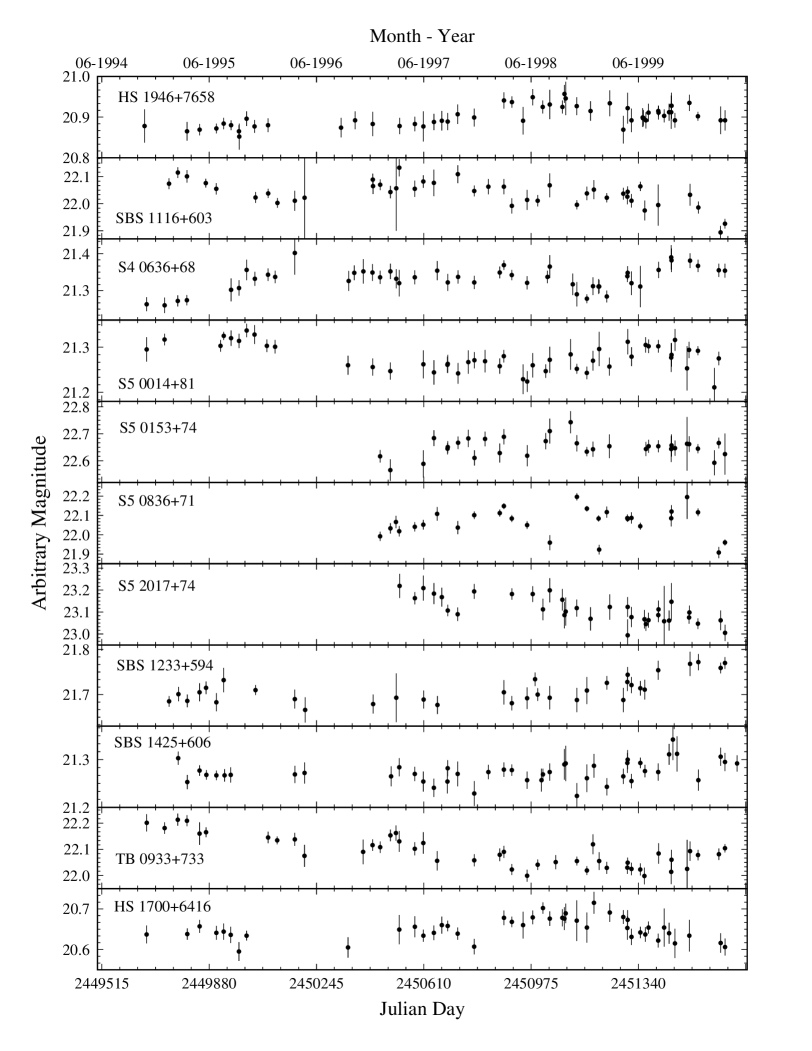
In spite of the difficulties we initiated a program to monitor high-luminosity quasars. Our sample consist of 11 quasars which were chosen to have high northern declination, redshift of 2 to 3.4 (to include the Ly and C iv UV lines in the optical region), and observed magnitudes in the range of 16–18 mag. The sample is being monitored photometrically in and bands each month at the WO since 1994 November. Preliminary results are presented in Figure 5. All 11 quasar show variations in the R-band flux of mag. The quasar S5 0836+71 has the largest variability which is mag. The variation of the high-luminosity quasars are smaller than the variations found for the PG quasars by about a factor of 5 in magnitude. While in a comparable time-period the variations in the PG quasars were in the range of 0.5–1 mag (Giveon et al. 1999) the typical variations of the high-luminosity quasars are only 0.1 mag. However, while the monitoring period is comparable in the observer time frame the rest-frame monitoring period of the high-luminosity quasars is about a factor of 4 smaller than the PG quasars monitoring period and only amounts to 1.5 years.
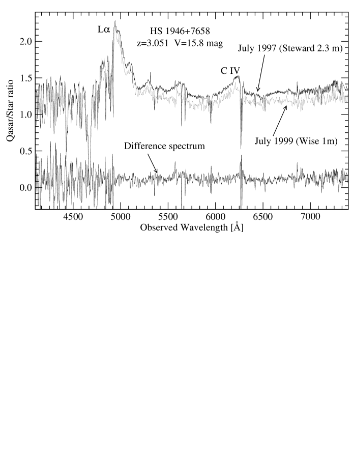
Spectrophotometric observations are needed in order to check a corresponding variations in the emission lines. We carried out few preliminary observations toward the brightest objects in the sample using the WO and SO telescopes. Our best observations are demonstrated in Figure 6. We present two observation epochs separated by two years, each with total integration time of 4 hours. The observing technique is, as described in section 2., of using a comparison star in the slit simultaneously with the quasar. During the 2 years period a continuum variation of about 10% is seen. This corresponds to the fading this object shown in the R-band photometry (Figure 5). No line variations is detected in the difference of the two spectra.
Figure 6 demonstrates that monitoring high-luminosity high-redshift quasars is feasible and interesting results can be obtained, however, it also demonstrates the difficulty to carry out such a monitoring using small to medium size telescopes. Even though the total integration time is 4 hours and the observing conditions are good the S/N of the spectra is poor. It is clear that a large telescope is needed to carry out this spectroscopic program. Early in 2000 we started monitoring a subsample of our 11 quasars with the 8 m Hobby-Eberly telescope which is partly owned by the Pennsylvania State University. We hope that within a short time we will be able to present preliminary results from this long term monitoring program.
6. Summary
We reviewed the final results from a spectrophotometric monitoring of a large, optically selected quasar sample (for the detailed study see Kaspi et al. 2000). We find time lags between the optical continuum and the Balmer-line light curves for all AGNs with adequate sampling. Our work doubled the number of AGNs with a measured time lag (i.e., BLR size). We also increased the available luminosity range for studying the size–mass–luminosity relations in AGNs from two to four orders of magnitude allowing, for the first time, to construct reliable relations. Using all AGNs with known BLR size we find that the BLR size scales with the 5100 Å luminosity as . This is significantly different from previous studies and is in contradiction with simple theoretical expectations, both suggesting . We also obtained a mass–luminosity relation for AGNs, , which, however, has a large intrinsic scatter. These findings impose new and strict limitations on theoretical considerations and constrain any theoretical models which attempt to explain the AGN phenomenon.
One of our major current goals is to further increase our knowledge about continuum and line variations and BLR size in high-luminosity quasars ( ergs s-1). To that end we are initiating a program to monitor a sample of 11 high-luminosity high-redshift quasars. We presented preliminary results of the continuum variations in those objects to be mag. Spectrophotometric observations of the sample is on the way and we hope that with 8 m class telescopes such as the Hobby-Eberly telescope we will be able in a few years to extend our knowledge about BLR size to the most luminous quasars. The conclusion of this long-term monitoring will hopefully complete the reverberation studies to cover the entire AGNs luminosity range of – ergs s-1.
Acknowledgments.
I deeply thank my collaborators in the PG quasars monitoring program Uriel Giveon, Buell Jannuzi, Dan Maoz, Hagai Netzer, and Paul Smith who spent years of work to achieve the results presented here. I would also like to thank my additional collaborator in the high-luminosity quasars monitoring program Niel Brandt, Donald Schneider, and Ohad Shemmer. Research at the WO is supported by grants from the Israel Science Foundation. Monitoring of PG quasars at SO was supported by NASA grant NAG 5-1630.
References
Alexander, T. 1997, in Astronomical Time Series, ed. D. Maoz, A. Sternberg & E. M. Leibowitz (Dordrecht: Kluwer), 163
Boroson, T. A., & Green, R. F. 1992, ApJS, 80, 109
Brandt, W. N., Laor, A., & Wills, B. J. 2000, ApJ, 528, 637
Dumont, A. -M., Collin-Souffrin, S., & Nazarova, L. 1998, A&A, 331, 11
Edelson, R. A., & Krolik, J. H. 1988, ApJ, 333, 646
Gaskell, C. M. 1988, ApJ, 325, 114
Gaskell, C. M. 1994, in Reverberation Mapping of the Broad-Line Region in AGN, ed. P. M. Gondhalekar, K. Horne & B. M. Peterson (San Francisco: ASP), 111
Gaskell, C. M., & Peterson, B. M. 1987, ApJS, 65, 1
Gaskell, C. M., & Sparke, L. S. 1986, ApJ, 305, 175
Giveon U., Maoz, D., Kaspi, S., Netzer, H., & Smith, P. S. 1999, MNRAS, 306, 637
Jackson, N., et al. 1992, A&A, 262, 17
Kaspi, S., Smith, P. S., Netzer, H., Maoz, D., Jannuzi, B. T., & Giveon, U. 2000, ApJ, 533, 631
Kellermann, K. I., Sramek, R., Schmidt, M., Shaffer, D. B., & Green, R. 1989, AJ, 98, 1195
Koratkar, A. P., & Gaskell, C. M. 1991a, ApJS, 75, 719
Koratkar, A. P., & Gaskell, C. M. 1991b, ApJ, 370, L61
Koratkar, A. P., Pian, E., Urry, C. M., & Pesce, J. E. 1998, ApJ, 492, 173
Korista, K. T. 1991, AJ, 102, 41
Laor, A, & Netzer, H. 1989, MNRAS, 238, 897
Laor A., Fiore, F., Elvis, M., Wilkes, B. J., & McDowell, J. C. 1997, ApJ, 477, 93
Maoz, D., & Netzer, H. 1989, MNRAS, 236, 21
Netzer, H., & Peterson, B. M. 1997, in Astronomical Time Series, ed. D. Maoz, A. Sternberg & E. Leibowitz (Dordrecht: Kluwer), 85
Neugebauer, G., Green, R. F., Matthews, K., Schmidt, M., Soifer, B. T., & Bennett, J. 1987, ApJS, 63, 615
O’Brien, P. T., & Gondhalekar, P. M. 1991, MNRAS, 250, 377
O’Brien, P. T., & Harries, T. J. 1991, MNRAS, 250, 133
Pérez, E., Penston, M. V., & Moles, M. 1989, MNRAS, 239, 55
Peterson, B. M. 1993, PASP, 105, 207
Peterson, B. M., & Wandel A. 1999, ApJL, 521, 95
Peterson, B. M., Wanders, I., Bertram, R., Hunley, J. F., Pogge, R. W., & Wagner, R. M. 1998a, ApJ, 501, 82
Peterson, B. M., Wanders, I., Horne, K., Collier, S., Alexander, T., Kaspi, S., & Maoz, D. 1998b, PASP, 110, 660
Peterson, B. M. et al. 1999, ApJ, 510, 207
Schmidt M., & Green, R. F. 1983, ApJ, 269, 352
Ulrich, M. H., Courvoisier, T. J.-L., & Wamsteker, W. 1993, ApJ, 411, 125
Wandel, A., Peterson, B. M., & Malkan M. A. 1999, ApJ, 526, 579
White, R. J., & Peterson, B. M. 1994, PASP, 106, 879
Wisotzki, L., Wucknitz, O., Lopez, S., & Sorensen, A. N. 1998, A&A, 339, L73
Zheng, W. 1988, ApJ, 324, 801
Zheng W., Kriss, G. A., Telfer. R. C., Grimes, J. P., & Davidsen A. P. 1997, ApJ, 475, 469