The Faint Sky Variability Survey I: An Overview

Abstract

The Faint Sky Variability Survey is aimed at finding variable objects in the brightness range between 17th and 25th magnitude on timescales between tens of minutes and years with photometric precisions ranging from 3 millimagnitudes for the brightest to 0.2 magnitudes for the faintest objects. An area of at least 50 square degrees, located at mid-galactic latitudes, will be covered using the Wide Field Camera on the 2.5m Isaac Newton Telescope on La Palma. The survey started in November 1998 as part of the INT Wide Field Survey program. Here we describe the main goals of the Faint Sky Variability Survey, the methods used in extracting the relevant information and the future prospects of the survey.

1 Introduction

The advance of large format ($>$2k$\times$2k) CCDs with high quantum efficiency has opened up a new area in Galactic and extragalactic astrophysics: the systematic study of astrophysical objects fainter than 20th magnitude. The importance of this brightness regime is nicely illustrated by the current, fast development in the field of Gamma-ray Bursts (GRBs; for recent reviews see Katz, Piran and Sari, 1998; Piran, 1999; and Van Paradijs, Kouveliotou and Wijers, 2000), where the localization of faint variable optical counterparts has led to a large increase in our understanding of gamma-ray bursts.

The Faint Sky Variability Survey (FSVS ) started in November 1998. This survey is aimed at finding variable objects in the brightness range between 17th and 25th magnitude on timescales between tens of minutes and years. In the following sections we will outline the main goals of the survey (Sect. 2), the INT Wide Field Camera (Sect. 3), the observing strategy (Sect. 4) and field selection (Sect. 5). After a short comparison with other, running surveys (Sect. 6), we will discuss ata reduction (Sect. 7), final data products (Sect. 8), availability of the data (Sect. 9) and a short overview of the current status of the Survey (Sect. 10). An overview of the general results of the first year of observations will be given in an accompanying paper (Everett et al., 2000).

2 Goals of the FSVS

Understanding the variability of stars has often been crucial in the development of astrophysics, with applications ranging from the evolution of stars, to the structure of our Galaxy and the distance scale of the Universe. Variability studies are currently mainly restricted to either bright regimes (brighter than 20th magnitude) or very small areas (supernovae and GRB searches). In the galactic realm, a deep variability study will not only reveal the characteristics of specific groups of stellar objects, but will also shed light on the outer parts of our Solar System, the direct Solar Neighbourhood, the structure of our Galaxy, and the extent of the Galactic Halo. The FSVS is aimed at observing at least 50 square degrees (50^□) down to 25th magnitude. The main targets can be divided into two broad areas of interest: photometrically and astrometrically variable objects.

2.1 Photometrically variable objects

Among the various classes of variables stars our main targets are:
$\bullet$ Close Binaries: Current detections of low-mass close-binary systems (Cataclysmic Variables, Low-mass x-ray binaries (including Soft X-ray Transients) and AM CVn stars) are strongly biased to small subsets of their populations. Of these systems the Cataclysmic Variables (CVs) form the main subgroup we expect to find. We refer to Warner (1995) for an extensive review of CV properties. Currently, most CVs are either found as by-products of extragalactic studies like blue-excess, quasar surveys (e.g. the Palomar-Green survey: Green, Schmidt and Liebert, 1986; the Hamburg(/ESO) Quasar Survey: Engels et al., 1994; Wisotzki et al., 1996; and the Edingburgh-Cape Survey: Stobie et al., 1988), or by their outbursts in which the system suddenly brightens 3-10 magnitudes due to an instability in the accretion disk. However, theoretical calculations show that the majority of the CV population should have evolved down to mass-transfer rates that are lower than $\sim$10^-11 M_⊙ yr^-1 (see e.g. Kolb 1993; Howell, Rappaport and Politano 1996; Howell, Nelson and Rappaport, 2000). At these very low-mass transfer rates CVs are expected to be faint (typically V$>$20), have no UV excess, show no (frequent) outbursts, and will therefore not show up in conventional searches. However, all CVs show intrinsic variability of the order of tenths of magnitudes or more. This variability is either caused by ‘flickering’ (mass-transfer instabilities), orbital modulations (hot-spots or eclipses) or long-term mass-transfer fluctuations. Searching for faint variable stars is therefore a very good way to disclose the characteristics of the majority of the CV population. The same search technique will also make the survey sensitive to other classes of close binaries, such as low-mass x-ray binaries, soft X-ray transients in quiescence and AM CVn stars. Since their space densities are much lower than that of CVs, we expect fewer of these in our Survey. However, because a much smaller number of these systems is known, even the discovery of a few can be a major contribution to the field.
$\bullet$ RR Lyrae: Due to their standard candle properties and easy recognition by colour and variability, RR Lyrae stars can be used as excellent tracers of the structure of the galactic halo. A few of these stars have been found at large galactocentric distances (Hawkins, 1984; Ciardullo et al., 1989), but number statistics are still poor. Finding more of these stars will help to constrain the total enveloped mass in the Galaxy at different radii.
$\bullet$ Optical Transients to Gamma-Ray Bursts The detection of optical counterparts to $\gamma$-ray bursts (GRBs, e.g. Van Paradijs et al., 1997), and the subsequent classification of GRBs as cosmological (e.g. Metzger et al., 1997, Kulkarni et al., 1998) have shown that GRBs are among the most energetic phenomena known in the Universe. The high energies implied by observations of GRB afterglows (10^53-54 erg in $\gamma$-rays if isotropy is assumed, Kulkarni et al., 1998; 1999), raises the question whether GRBs are emitting their energy isotropically or in the form of jets. In the latter case the energies involved will be much lower, depending on the amount of beaming. Even if the $\gamma$-rays are beamed the optical afterglow is expected to radiate more isotropically, and thus one expects to observe faint afterglows without an accompanying burst in $\gamma$-rays. Detections or non-detections of such transient events will constrain the beaming angle. A discussion and analysis of such results will be presented in Vreeswijk et al. (2001).

2.2 Astrometrically variable objects

The observing schedule that we have adopted for the FSVS (see Sect. 4) also allows for the detection of astrometrically variable objects. Our interests fall into two main categories:
$\bullet$ Kuiper Belt Objects: Kuiper Belt Objects (KBOs) are icy bodies revolving around the Sun in orbits that lie outside the orbit of Neptune (which has led to the alternative name of Trans Neptunian Objects; TNOs). Since their discovery in 1993 (Jewitt and Luu, 1993), more than 100 of these objects have been found. Studying their properties will give important insight into the formation of the Solar system and planetary systems in general. One question that is particularly well suited to be answered is the inclination distribution of KBOs. Most KBOs have been found within 5^∘ from the ecliptic, but this may constitute an observational bias, since most searches have been (and are) performed close to the ecliptic. Since the FSVS is mostly pointing away from the ecliptic, we will be able to set limits on the inclination distribution of KBO’s.
$\bullet$ Solar Neighbourhood Objects: The planned re-observations after one year will allow for the detection of high proper-motion objects in the Solar neighbourhood. These will be extremely important to constrain the low-mass end of the IMF in the solar neighbourhood, to estimate the relative contribution of the disk and halo population of stars in the solar neighbourhood and trace the star formation history of the galactic halo by finding old, high proper motion, white dwarfs. It may also serve as a powerful tool to find nearby solitary field brown dwarfs.

3 The INT Wide Field Camera

The Wide Field Camera (WFC) is mounted at the prime focus of the 2.5m Isaac Newton Telescope (INT) on the island of La Palma. The WFC consists of 4 EEV42 CCDs, each containing 2048$\times$4100 pixels. They are fitted in an L-shaped pattern, which makes the Camera 6k$\times$6k, minus a 2k$\times$2k corner (see Figure 1). The CCDs consist of 13.5$\mu$ pixels (0$.\!\!^{\prime\prime}$33 per pixel on the sky), which gives a sky coverage per CCD of 22$.\mkern-4.0mu^{\prime}$8$\times$11$.\mkern-4.0mu^{\prime}$4. A total of 0$.\!\!^{\Box}$29 is covered by the combined four CCDs. With a typical seeing of 1$.\!\!^{\prime\prime}$0-1$.\!\!^{\prime\prime}$3 on the INT, point objects are well-sampled, which allows for accurate photometry. The Camera is equiped with a filter set consisting of Harris B,V and R, RGO U, I and Z filters and Sloan g^′,r^′,i^′ filters. Zeropoints, defined as the magnitude that gives 1 detected e^-/s, of the instrument are 25.6 in B,V and R, 23.7 in U and 25.0 in I.

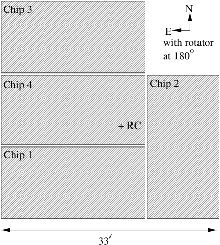
Figure 1: Graphical lay-out of the WFC 4 EEV 4k$\times$2k CCDs. In the orientation used by the FSVS, North is up and East is to the left. The WFC rotates around its Rotator Center (RC).

4 Observing strategy

The typical timescales of variability covered by the objects listed above vary from hours (CVs, KBOs, RR Lyraes) to days (Optical transients to GRBs) to years (high proper motion stars). To cover all possible timescales of variation we have devised an observing strategy that optimises both the coverage per field as well as the total sky coverage. The variability search is done in the V-band filter. This is an optimum between the expected colours of our sources (blue as well as red, sensitivity of the WFC (peaks in B and V) and the coverage of the optical band with three filters, for which we have chosen the B and I-band filters to obtain colour information. For the photometric variability we find that at least 15-20 pointings are needed to firmly state that an object is variable and also get an indication of the timescale of its variability (or ideally its period). For the first two runs of the FSVS this number was limited to $\sim$12, but has been raised to 15-20 in subsequent runs. For the first two years the FSVS has been allocated one week of dark time per semester. Since each observing run consists of six to seven consecutive nights of dark time, the 15-20 pointings per field have to be distributed over these nights. One of the criteria for the selection of the fields (see Sect. 5) is the fact that we want to observe each field within 30^∘ of the zenith. Per night this gives an effective time-slot of three hours to observe a particular field. We have chosen to observe the fields within 30^∘ of the zenith to minimize the effect of differential refraction on the differential photometry and astrometry used to determine the light curve and proper motions of each object.

These considerations have led to a semi-logarithmic observing sequence in which all possible time-scales are sample. The exact order of observations within the observing period depends on when a photometric night occurs. It is on these nights that the photometric calibration and field observations in B and I are done, along with two observations in V. Integration times are 10 minutes in B and V and 15 minutes in I. Combined with the observing schedule outlined above, this means that per three hour period three different fields can be observed. In a six night run it is possible to observe two sets of fields, that have an intertwining observing schedule. In practice this means that for observations in, for instance, November, when nights have 9-10 hours of dark time, we can observe 2 (sets of fields)$\times$3 (observing slots per night)$\times$3 (fields within one slot) = 18 fields in total. In November 1998 we were able to cover 18 fields (=5$.\!\!^{\Box}$22). In May 1999 and May 2000, when observing nights were only 6-7 hours, we covered 12 fields (3$.\!\!^{\Box}$48) each. After a year each field is re-observed, enabling the search for long-term photometric variability and high-proper motion objects.

5 Field selection

The field selection is governed by the following four criteria (in order of importance), which have been set to ensure maximum quality of the data:

• Fields are located between Galactic latitude 20^∘$<b^{II}<$ 40^∘: to probe the Galactic halo as well as the Galactic disk to considerable depths we target our fields at mid-Galactic latitudes. This also prevents problems with field crowding and interstellar extinction that will be present at lower Galactic latitudes. The field crowding would limit the accuracy of the differential photometry, especially for faint objects. The main effect of interstellar extinction would be to limit the distance to which we are able to observe into the halo.

• Fields are observed within a zenith distance, $z<$30^∘: this criterion has been set to ensure that the effect of differential extinction coefficients has no impact on the accuracy with which the differential photometry can be done.

• If possible we will point our fields at the ecliptic, to increase the chances of finding KBOs. However, as explained in Sect. 2.2 even if we are not able to point at the ecliptic, our results may help to constrain the inclination distribution of KBOs.

• Bright stars are avoided: stars brighter than $\sim$10th magnitude will cause large charge overflows and diffraction patterns that limit the area on a CCD that can be used for accurate photometry, depending on the placement and brightness of the star. To prevent this from happening the fields are selected to be as devoid as possible of bright stars. We checked for the presence of bright stars using the DSS in the selection of the fields.

It is clear that not all four criteria can be met at all times of the year. For the northern Hemisphere all four criteria are only satisfied in late November-early December.

6 Comparison with other surveys

The FSVS is unique in its search for variability on short timescales (tens of minutes to days), depth and precision of its differential photometry, although having a rather moderate sky-coverage. The Sloan Digital Sky Survey (SDSS) covers a much larger area of the sky (10 000 ^□), but at brighter magnitudes (14 $<g^{\prime}<$ 22.5), and provides almost no variability information. The microlensing studies (e.g. MACHO, Alcock et al., 1997; EROS, Beaulieu et al., 1995) do obtain variability information, but are targeted at different stellar populations (the Galactic Bulge, the LMC, or M31) and have a limit of V$\sim$21 with a photometric precision of 0.5 mag at the faint end, caused by limited S/N and crowding in their necessarily high density star fields. Supernovae searches reach as deep as the FSVS, but have a much lower time-resolution. In Figure 2 we show schematically how the FSVS compares with other deep ongoing surveys.

Figure 2: A comparison in area and depth between major current surveys and the FSVS. Adapted from the NOAO Deep Survey Web-pages (see http://www.noao.edu/noao/noaodeep/; SDSS=Sloan Digital Sky Survey; BTC50 = Survey of Falco et al.; EIS(deep) = ESO Imaging Survey (Deep); Deeprange = Postman et al I-band survey; HawDS= Hawking Deep Survey; HDF= Hubble Deep Field; NOAO= NOAO Survey; CFRS = Canada France Redshift Survey ; CADIS = Calar Alto Deep Imaging Survey; CFDF = Canadian French Deep Fields). Note that most of these surveys have no or very limited variability information. The range in depth for the FSVS is reached by using each individual image (as in the variability study) or the sum images.

7 Reduction and Analysis Methods

To obtain variability information on all the objects detected in our observations we use the technique of differential aperture photometry. We have written a pipe-line reduction package, consisting of IRAF tasks, Fortran programs and at its core the SExtractor program by Bertin and Arnouts (1996). Every object in every observation is analysed and the results are stored in a master-table that lists the essential information (described below in detail) for each object. When a photometric calibration is available, the colours of each object are determined and written to the master-table. Below we outline the data flow through our pipe-line reduction, starting with the raw data as it comes from the telescope.

7.1 Bias subtraction

The mean of the counts in the overscan region of each observation is used to subtract the overall bias level. After this the 2-D bias pattern, determined from bias observations taken at the start of the night, is subtracted.

7.2 Linearization of the data

A non-linearity in the read-out electronics causes all data taken with the INT WFC to be non-linear up to a level of $\sim$5%. The magnitude of this non-linearity as a function of exposure level is determined by the Cambridge WFS group and is posted in tabular and analytic form. These corrections are applied after bias-subtraction.

7.3 Flatfielding

From twilight skyflats taken during a whole observing run a master flatfield is made, which is used for all the observations taken in that band during the observing run. For the I-band observations, which suffer from fringing at the 3.5% level, we have made fringe maps from the night time observations, which allows the fringe pattern to be removed down to the 0.6% continuum sky level (see Fig. 3).

Figure 3: Defringing of the I-band observations, using a fringe map made from the night-time observations themselves. Left: Before defringing, middle: fringe map, right: after defringing

7.4 Source detection

The bias-subtracted, linearized and flatfielded data are fed to the SExtractor program. This program detects sources and measures their instrumental magnitude in a number of different ways, as set by the user. Source detection is done by requiring that three neighbouring pixels are more than two sigma above the sky-background. Visual inspection shows that this threshold value is capable of detecting virtually all objects that can be identified by eye. Some contamination from extended cosmic rays is present, but these are effectively removed in the subsequent steps. Apart from finding the sources and determining their instrumental magnitudes, for each source the SExtractor program determines various other parameters such as its position, size, extent, ellipticity and orientation angle. Due to vignetting a corner of CCD3 (the NE corner in Fig. 1) has very low count rates. We discard any object detected in a square box 200 pixels wide from this corner of CCD3.

7.5 Instrumental magnitudes

From bright, unsaturated objects detected in the central 1k$\times$1k pixels of each CCD the seeing is determined from the median of the distribution of 2-D Gaussian fits to those objects. This seeing parameter is used to set the sizes of our photometry apertures for each exposure. We measure the objects in four apertures having radii of 0.5, 1.0, 1.5 and 2.0 times the seeing FWHM. These radii are chosen to sample around the optimal S/N radios of 1.3$\times$the seeing FWHM. However, depending on the object’s brightness a smaller or larger aperture than this optimal value may be applicable. We leave it to the user to choose the aperture most suited for the topic under investigation. Errors are calculated from the photon counting statistics.

Using aperture photometry ofcourse relies on an accurate background subtraction around each object. This fails when field crowding becomes severe. However, even in the most crowded field (taken at a galactic latitude, $b^{\sc ii}\sim$20^∘), the density of objects is still low enough for good aperture photometry to be applied. We illustrate this in Fig. 4, which shows the detection histogram for one CCD in one of our lower galactic latitude fields. We detect $\sim$2300 objects with $V<$24 in this image. With an average seeing of 1$.\!\!^{\prime\prime}$2, each object occupies roughly 16 pix. In total these objects will therefore cover about 3.7$\times$10³ pix, a very small fraction,$<0.5$%, of the total area available on the CCD.

Figure 4: Histogram of the number of objects per magnitude for one CCD in one of our lower galactic latitude fields. In total we detect $\sim$2300 objects with $V<$24.

7.6 Field matching

Different observations of the same field are automatically matched using the offset program, supplied with the dophot package (Schechter, Mateo and Saha; 1993), using the 100 brightest, non-saturated stars, that are not located near the edges of the CCDs. Matching is done by triangle pattern recognition in the two images. This matching allows for linear scaling, rotation and translation of the different images. Output is given as the elements of a rotation-translation matrix. All images are transformed to one of the images that is taken as a reference image (typically the one with the best seeing). Individual objects are matched if in the new image an object is found within 1 FWHM of the position of the object in the reference image. Given the low density of objects in our images the chances of an incorrect matching are very low. This same criterion is used to match stars between different filters.

7.7 Local reference star selection

In order to obtain differential magnitudes, an ensemble of local reference stars has to be selected. The average (ensemble) magnitude of these stars is used to compute all instrumental magnitudes. In the selection of this ensemble it is important to use the brightest, non-variable, stars that are not saturated. Using the brightest stars is essential because the error on the differential magnitude of any object consists of the error that is obtained from counting statistics for that object, and the error on the average of the reference stars (see e.g. Howell, Mitchell and Warnock, 1988). The uncertainty in the mean magnitude of the ensemble must be made significantly smaller than the uncertainty imposed by counting statistics on the magnitude of any star of interest. If this is not the case, it will cause small-amplitude variability, that should have been detected on the basis of counting statistics, to become undetectable. Currently, per CCD, an ensemble of at least ten local standards is selected by requiring that their variation with respect to the average is less than 5 millimagnitudes. If this requirement is set more stringently not enough standards are found. In the North Galactic Pole observations of May 1999 the selection criterion had to be relaxed to 10 millimagnitudes in order to find a suitable number of stars. This is, of course, due to the limited number of stars in the NGP direction. As explained above, this selection criterion naturally sets the minimum amplitude of variation that can be found.

7.8 Differential magnitudes

For every object the differential magnitude is calculated against the ensemble average. The error of the instrumental magnitude is propagated to the differential magnitude, adding quadratically the error on the ensemble average. The differential magnitude is calculated for all four aperture size as described in Sect. 7.5.

7.9 Absolute calibration

Using the USNO A2.0 catalogue an astrometric solution is obtained for each CCD and each field separately. On average, each CCD contains 20-30 USNO A2.0 stars, which is sufficient to obtain a cubic solution that is accurate to 0$.\!\!^{\prime\prime}$2-0$.\!\!^{\prime\prime}$4 in right ascension and declination, depending on the position of a field on the sky.

During all our runs so far, we have had two photometric nights, during which all fields and several Selected Areas of Landolt (1992) were observed. After having found the astrometric solution, we can measure the standard stars automatically, now knowing where they are located, using their position in the Landolt catalogue. We use the SExtractor aperture photometry option, with an aperture radius of twice the image FWHM. For each CCD the measured BVI standard star magnitudes are fit with a model that includes a zero-point offset, an airmass term and a colour term. When sufficient standards are observed at different airmasses, we fit for the airmass term. If not, we hold it constant at the following values: 0.25, 0.15 and 0.07 for the filters B, V and I, respectively. The colour term is only included if it improves the fit significantly. These solutions are applied to all objects listed in the catalogue through the reference stars that are selected for each CCD of each field (see Sect. 7.7). We estimate the error in the absolute calibration to be 0.05 for the B and V filters, and 0.1 for the I band.

7.10 Limiting magnitudes

Based on the amount of flux in the ten reference stars (see Sect. 7.7), the level of the background sky, the photometry aperture size and the background aperture size, we calculate the flux a 3-, 5-, and 7-sigma object would have for each CCD, field and observation. These ten estimates of the 3-,5- and 7-sigma limits are then averaged to produce an average 3-, 5- and 7-sigma limiting magnitude. In this calculation we neglect the read-out noise since our observations are long and have background levels whose noise is much higher than the read-out noise.

7.11 Variability

Variability of an object is determined on the basis of the differential magnitudes discussed above. The mean of the differential light curve of each object. This constant fit returns a $\chi^{2}$-value, the magnitude of which is taken as a measure of the object’s variability. In case an object is not detected in an observation, that observation’s limiting magnitude is taken as an upper limit to the brightness of the object.

7.12 Star- Galaxy seperation

The star-galaxy separation used in the FSVS is based on the ’stellarity’ parameter, as returned from the SExtractor routines (Bertin and Arnouts, 1996). This parameter has a value between 0 (highly extended) and 1 (point source). In the FSVS the stellarity value of an object is taken as the value in the combined V-band images. Due to the increased S/N is this image, the star-galaxy separation can be done reliably almost 1 magnitude deeper than from any individual image. As can be seen in Fig. 5 this seperation of object types works very well to classify stars (with a value $>$0.8) down to V$\sim$23.5-24). Fainter stars tend to have slightly lower stellarity values (the turn down between 23 and 24) but can still be well separated from the galaxies.

Figure 5: The stellarity versus magnitude for one CCD in one of our fields. A stellarity of zero indicates a highly extended source, and a stellarity of one is a point-source. Different symbols represent different observations. The lower stellarity of point-sources at the bright end of our magnitude range is caused by saturation. Detections at V$>$25 are noise spikes.

7.13 Astrometric data-analysis and search for Kuiper Belt Objects

The search for Kuiper Belt Objects is made using the moving object detection code of one of us (HS). This code is tuned to the particular photometric properties of the data frames in question as well as to the expected range of rate of motion for KBOs in that area of the sky. The signal-to-noise cutoff is selected to find the maximum number of real objects while keeping the rate of false detections to a manageable level.

Three, or ideally four images, taken at different times during the same night are scanned by the Scholl code to identify all ”stellar” objects on the frames and match them across frames. Those with rates of motion within the target range are flagged and small cutouts of the CCD frames including each of the flagged objects are automatically prepared. These are blinked by a human operator to confirm the detections of real objects and remove false detections.

Once the real detections have been flagged, the code performs astrometry on the objects using the USNO catalogue. The resulting astrometry is ready for reporting to the Minor Planet Center and for follow-up observations.

8 Final products

The pipeline discussed above returns two sets of output files:
$\bullet$ The reduced images
$\bullet$ The data tables with the photometric and astrometric information.
The data tables are made per field, per CCD and are made for four different apertures: 0.5, 1.0, 1.5 and 2.0 $\times$FWHM, where the FWHM is defined as the average full width at half maximum of the stellar profiles in the central 1k$\times$1k part of each CCD and each exposure.

The data tables contain, for all the detected objects, the information on the time of observation, name, position and colour for each object, followed by the magnitude, error on the magnitude, fwhm, stellarity and the error flag as returned from the SExtractor program for each object and each observation.

If an object is only detected in a subset of all the observations, it is added to the final catalogue, and dummy values are introduced when it was not detected.

The objects names are given in standard IAU format as FSVSJhhmmss.ss+ddmmss.s, all in J2000 coordinates. Each object is also given an ’internal’ name whose format is F_XX_Y_ZZZZZ, with XX the field number, Y the CCD number (1-4) and ZZZZZ a five digit detection number. The position of each object is given both in RA and DEC as well as in x,y-coordinates in the reference frame of the specific field.

9 Availability of the data

All raw data is available upon request from the ING-WFS archive in Cambridge after the one year propietary right. For UK and NL astronomers the data is immediately available. All data-tables, containing the reduced information described above, are retrievable from the FSVS-website.

10 First year observations

An extensive discussion of the results from the first year of observations is given in Paper II and is outside the scope of this paper. However, observing conditions in the first two runs of the FSVS have been good and data is now available for a total of 30 fields (8$.\!\!^{\Box}$7). As will be discussed in Paper II, using the pipe-line reduction as described above, point source light curves have been obtained with photometric precisions as good as a few millimag for the brightest (V$\sim$17) sources. At 24th magnitude precision on the differential photometry is still in the 0.1-0.15 mag range.

11 Conclusions

The FSVS offers a unique possibility of studying the behaviour of variable objects in the magnitude range of 17 $<V<$ 25 with photometric precisions ranging from 3 millimag (at $V$=17) to 0.15 mag (at V$\simeq$24). Observations in the first year show that the FSVS is producing promising results.

Besides the study of variable objects, the FSVS offers a large dataset that can serve as the basis for many research topics (e.g. YSO’s, gravitational lenses, galaxy counts, quasar searches). The FSVS-collaboration encourages the use of the data set for purposes other than the ones mentioned here.

References

- [1997] Alcock, C., et al., 1997, ApJ 486, 697
- [1995] Beaulieu, J.P., et al., 1995, A&A 303, 137
- [1996] Bertin, E. and Arnouts, S., 1996, A&AS 117, 393
- [1989] Ciardullo, R., Jacoby, G.H., Bond, H.E., 1989, AJ 98, 1648
- [1994] Engels, D., Cordis, L., Köhler, T., 1994, in IAU Symp. 161, eds. H.T. MacGillivray et al. (Kluwer, Dordrecht), p. 317
- [1999] Everett, M., et al., 2000, same issue (Paper II)
- [1986] Green, R.F., Schmidt, M. and Liebert, J., 1986, ApJS, 61, 305
- [1984] Hawkins, M.R.S., 1984, MNRAS 206, 433
- [1988] Howell, S.B., Mitchell, K.J and Warnock, A., 1988, AJ 95, 247
- [1997] Howell, S.B., Rappaport, S. and Politano, M.R., 1997, MNRAS 287, 929
- [2000] Howell, S.B., Nelson, L. and Rappaport, S., 2000, ApJ, in press
- [1993] Jewitt, D. and Luu, J., 1993, Nature 362, 730
- [1998] Katz, J.I, Piran, T. and Sari, R., 1998, Phys. Review Letters, 80, 1580
- [1993] Kolb, U., 1993, A&A 271, 149
- [1998] Kulkarni, S.R., et al., 1998, Nature 393, 35
- [1999] Kulkarni, S.R., et al., 1999, Nature 398, 389
- [1997] Metzger, M.,R., et al., 1997, Nature 387, 878
- [1999] Piran, T., 1999, Physics Reports, in press
- [1993] Schechter, P.L., Mateo, M. and Saha, A., 1993, PASP 105,1342
- [1988] Stobie, R.S., Morgan, D.H., Bhathia, R.K., Kilkenny, D. and O’Donoghue, D., 1988, in The Secnd Conference on Faint Blue Stars, IAU Colloq. 95,eds. D. Philip et al., David Press, Schenectady, NY, p. 43
-
[1997]
Van Paradijs, J., Groot, P.J., Galama, T.J et al., 1997, Nature 368, 686
- [2000] Van Paradijs, J., Kouveliotou, Ch. and Wijers, R.A.M.J., 2000, ARA&A in press
- [2001] Vreeswijk, P.M. et al., 2001, A&A, in preparation
- [1995] Warner, B., 1995, Cataclysmic Variables, Cambridge Astrophysics Series 28, CUP, Cambridge, UK.
- [1996] Wisotzki, L., Köhler, T., Groote, D and Reimers, D., 1996, A&AS 115, 227