UMN-TH-1923/00
TPI-MINN-00/47
CERN-TH/2000-287
astro-ph/0009475
September 2000 Big Bang Nucleosynthesis
and Related Observations

Abstract

The current status of big bang nucleosynthesis is summarized. Particular attention is paid to recent observations of ⁴He and ⁷Li and their systematic uncertainties. Be and B are also discussed in connection to recent ⁷Li observations and the primordial ⁷Li abundance.

1 Introduction

The simplicity of the standard model of Big Bang Nucleosynthesis (BBN) and its success when confronted with observations place the theory as one of the cornerstones of modern cosmology. BBN is based on the inclusion of an extended nuclear network into a homogeneous and isotropic cosmology. Apart from the input nuclear cross sections, the theory contains only a single parameter, namely the baryon-to-photon ratio, $\eta$. Other factors, such as the uncertainties in reaction rates, and the neutron mean-life can be treated by standard statistical and Monte Carlo techniqueskr ; hata1 ; sark2 ; bn . The theory then allows one to make predictions (with specified uncertainties) of the abundances of the light elements, D, ³He, ⁴He, and ⁷Li. As there exist several detailed reviews on BBN, I will briefly summarize the key results and devote this contribution to the impact of recent observations of ⁴He and ⁷Li along with the related observations of Be and B. In referring to the standard model, I will mean homogeneous nucleosynthesis, with three neutrino flavors ($N_{\nu}=3$), and a neutron mean life of 886.7 $\pm$ 1.9 s RPP .

The dominant product of big bang nucleosynthesis is ⁴He, resulting in an abundance of close to 25% by mass. Lesser amounts of the other light elements are produced: D and ³He at the level of about $10^{-5}$ by number, and ⁷Li at the level of $10^{-10}$ by number. The resulting abundances of the light elements are shown in Figure 1, over the range in $\eta_{10}=10^{10}\eta$ between 1 and 10. The curves for the ⁴He mass fraction, $Y$, bracket the computed range based mainly on the uncertainty of the neutron mean-life. Uncertainties in the produced ⁷Li abundances have been adopted from the results in Hata et al.hata1 . Uncertainties in D and ³He production are small on the scale of this figure. The dark shaded boxes correspond to the observed abundances and will be discussed below.

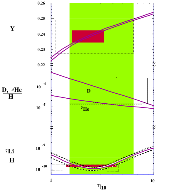
Figure 1: The light element abundances from big bang nucleosynthesis as a function of $\eta_{10}$.

At present, there is a general concordance between the theoretical predictions and the observational data, particularly, for ⁴He and ⁷Lifo . These two elements indicate that $\eta$ lies in the range $1.55<\eta<4.45$. There is limited agreement for D/H as well, as will be discussed below. High D/H narrows the range to $1.5<\eta<3.4$ and low D/H is compatible at the $2\sigma$ level in the range $4.2<\eta<5.3$.

2 Data

2.1 ⁴He

The primordial ⁴He abundance is best determined from observations of HeII $\rightarrow$ HeI recombination lines in extragalactic HII (ionized hydrogen) regions. There is a good collection of abundance information on the ⁴He mass fraction, $Y$, O/H, and N/H in over 70 such regionsp ; iz ; it . Since ⁴He is produced in stars along with heavier elements such as Oxygen, it is then expected that the primordial abundance of ⁴He can be determined from the intercept of the correlation between $Y$ and O/H, namely $Y_{p}=Y({\rm O/H}\to 0)$. A detailed analysis fdo2 of the data found

$$Y_{p}=0.238\pm 0.002\pm 0.005$$ (1)

The first uncertainty is purely statistical and the second uncertainty is an estimate of the systematic uncertainty in the primordial abundance determination. The solid box for ⁴He in Figure 1 represents the range (at 2$\sigma_{\rm stat}$) from (1). The dashed box extends this by including the systematic uncertainty. The He data is shown in Figure 2.

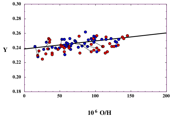
Figure 2: The Helium (Y) and Oxygen (O/H) abundances in extragalactic HII regions, from refs. p and from ref. it . Lines connect the same regions observed by different groups. The regression shown leads to the primordial ⁴He abundance given in Eq. (1).

The helium abundance used to derive (1) was determined using assumed electron densities $n$ in the HII regions obtained from SII data. Izotov, Thuan, & Lipovetsky iz proposed a method based on several He emission lines to “self-consistently” determine the electron density. Their data using this method yields a higher primordial value

$$Y_{p}=0.244\pm 0.002\pm 0.005$$ (2)

As one can see, the resulting primordial ⁴He abundance shows significant sensitivity to the method of abundance determination, leading one to conclude that the systematic uncertainty (which is already dominant) may be underestimated. Indeed, the determination (1) of the primordial abundance above is based on a combination of the data in refs. p , which alone yield $Y_{p}=0.228\pm 0.005$, and the data of ref. it (based on SII densities) which give $0.239\pm 0.002$. The abundance (2) is based solely on the self-consistent method yields and the data of it . One should also note that a recent determination piem of the ⁴He abundance in a single object (the SMC) also using the self consistent method gives a primordial abundance of 0.234 $\pm$ 0.003 (actually, they observe $Y=0.240\pm 0.002$ at [O/H] = -0.8, where [O/H] refers to the log of the Oxygen abundance relative to the solar value, in the units used in Figure 2, this corresponds to $10^{6}$O/H = 135). Therefore, it will useful to discuss some of the key sources of the uncertainties in the He abundance determinations and prospects for improvement. To this end, I will briefly discuss, the importance of reddening and underlying absorption in the H line line measurements, Monte Carlo methods for both H and He, and underlying absorption in He.

The He abundance is typically quoted relative to H, e.g., He line strengths are measured relative to $H\beta$. The H data must first be corrected for underlying absorption and reddening. Beginning with an observed line flux $F(\lambda)$, and an equivalent width $W(\lambda)$, we can parameterize the correction for underlying stellar absorption as

$$X_{A}(\lambda)=F(\lambda)({W(\lambda)+a)\over W(\lambda)})$$ (3)

The parameter $a$ is expected to be relatively insensitive to wavelength. A reddening correction is applied to determine the intrinsic line intensity $I(\lambda)$ relative to $H\beta$

$$X_{R}(\lambda)={I(\lambda)\over I(H\beta)}={X_{A}(\lambda)\over X_{A}(H\beta)}10^{f(\lambda)C(H\beta)}$$ (4)

where $f(\lambda)$ represents an assumed universal reddening law and $C(H\beta$) is the correction factor to be determined. By minimizing the differences between $X_{R}(\lambda)$ to theoretical values, $X_{T}(\lambda)$, for $\lambda=H\alpha,H\gamma$ and $H\delta$, one can determine the parameters $a$ and $C(H\beta)$ self consistently osk , and run a Monte Carlo over the input data to test the robustness of the solution and to determine the systematic uncertainty associated with these corrections.

In Figure 3 osk , the result of such a Monte-Carlo based on synthetic data with an assumed correction of 2 Å for underlying absorption and a value for $C(H\beta)=0.1$ is shown. The synthetic data were assumed to have an intrinsic 2% uncertainty. While the mean value of the Monte-Carlo results very accurately reproduces the input parameters, the spread in the values for $a$ and $C(H\beta)$ are considerably larger than one would have derived from the direct $\chi^{2}$ minimization solution due to the covariance in $a$ and $C(H\beta)$.

Figure 3: A Monte Carlo determination of the underlying absorption $a$ (in Å ), and reddening parameter $C(H\beta)$, based on synthetic data.

The uncertainties found for $H\beta$ must next be propagated into the analysis for ⁴He. We can quantify the contribution to the overall He abundance uncertainty due to the reddening correction by propagating the error in eq. (3). Ignoring all other uncertainties in $X_{R}(\lambda)=I(\lambda)/I(H\beta)$, we would write

$${\sigma_{X}\over X}=\ln 10~{}f(\lambda)~{}\sigma_{C(H\beta)}$$ (5)

In the example discussed above, $\sigma_{C(H\beta)}\sim 0.04$ (from the Monte Carlo), and values of $f$ are 0.237, 0.208, 0.109, -0.225, -0.345, -0.396, for He lines at $\lambda\lambda$3889, 4026, 4471, 5876, 6678, 7065, respectively. For the bluer lines, this correction alone is 1 – 2 % and must be added in quadrature to any other observational errors in $X_{R}$. For the redder lines, this uncertainty is 3 – 4 %. This represents the minimum uncertainty which must be included in the individual He I emission line strengths relative to H$\beta$.

Next one can perform an analogous procedure to that described above to determine the ⁴He abundance osk . We again start with a set of observed quantities: line intensities $I(\lambda)$ which include the reddening correction previously determined along with its associated uncertainty which includes the uncertainties in $C(H\beta)$; the equivalent width $W(\lambda)$; and temperature $t$. The Helium line intensities are scaled to $H\beta$ and the singly ionized helium abundance is given by

$$y^{+}(\lambda)={I(\lambda)\over I(H\beta)}{E(H\beta)\over E(\lambda)}({W(\lambda)+a_{HeI}\over W(\lambda)}){1\over(1+\gamma)}{1\over f(\tau)}$$ (6)

where $E(\lambda)/E(H\beta)$ is the theoretical emissivity scaled to $H\beta$. The expression (6) also contains a correction factor for underlying stellar absorption, parameterized now by $a_{HeI}$, a density dependent collisional correction factor, $(1+\gamma)^{-1}$, and a flourecence correction which depends on the optical depth $\tau$. Thus $y^{+}$ implicitly depends on 3 unknowns, the electron density, $n$, $a_{HeI}$, and $\tau$.

One can use 3-6 lines to determine the weighted average helium abundance, $\bar{y}$. From ${\bar{y}}$, we can calculate the $\chi^{2}$ deviation from the average, and minimize $\chi^{2}$, to determine $n,a_{HeI}$, and $\tau$. Uncertainties in the output parameters are also determined. In principle, under the assumption of small values for the optical depth $\tau$(3889), it is possible to use only the three bright lines $\lambda$4471, $\lambda$5876, and $\lambda$6678 and still solve self-consistently for He/H, density, and $a_{HeI}$. Of course, because these lines have relatively low sensitivities to collisional enhancement, the derived uncertainties in density will be large.

The addition of $\lambda$7065 was proposed iz as a density diagnostic and then, $\lambda$3889 was later added to estimate the radiative transfer effects (since these are important for $\lambda$7065). Thus the five line method has the potential of self-consistently determining the density and optical depth in the addition to the ⁴He abundance. The procedure described here differs somewhat from that proposed in iz , in that the $\chi^{2}$ above is based on a straight weighted average, where as in iz the difference of a ratio of He abundances (to one wavelength, say $\lambda$4471) to the theoretical ratio is minimized. When the reference line is particularly sensitive to a systematic effect such as underlying stellar absorption, this uncertainty propagates to all lines this way.

Adding $\lambda$4026 as a diagnostic line increases the leverage on detecting underlying stellar absorption. This is because the $\lambda$4026 line is a relatively weak line. However, this also requires that the input spectrum is a very high quality one. $\lambda$4026 is also provides exceptional leverage to underlying stellar absorption because it is a singlet line and therefore has very low sensitivity to collisional enhancement (i.e., $n$) and optical depth (i.e., $\tau$(3889)) effects.

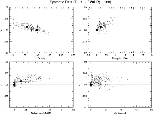
Figure 4: Results of modeling of 6 synthetic He I line observations. The four panels show the results of a density = 100 cm^-3, $a_{HeI}$ = 0, and $\tau$(3889) $=$ 0 model.

As in the case of the hydrogen lines, Monte-Carlo simulation of the He data can be used to test the robustness of the solution for $n,a_{HeI}$, and $\tau$ osk . Figure 4 presents the results of modeling of 6 synthetic He I line observations. The four panels show the results of a density = 100 cm^-3, $a_{HeI}$ = 0, and $\tau$(3889) $=$ 0 model. The solid lines show the input values (e.g., He/H = 0.080) for the original calculated spectrum. The solid circles (with error bars) show the results of the $\chi^{2}$ minimization solution (with calculated errors) for the original synthetic input spectrum. The small points show the results of Monte Carlo realizations of the original input spectrum. The solid squares (with error bars) show the means and dispersions of the output values for the $\chi^{2}$ minimization solutions of the Monte Carlo realizations.

Figure 4 demonstrates several important points. First, the $\chi^{2}$ minimization solution finds the correct input parameters with errors in He/H of about 1% (less than the 2% errors assumed on the input data, showing the power of using multiple lines). There is a systematic trend for the Monte Carlo realizations to tend toward higher values of He/H. This is because, the inclusion of errors has allowed minimizations which find lower values of the density and non-zero values of underlying absorption and optical depth. Note that the size of the error bars in He/H have expanded by roughly 50% as a result. We can conclude from this that simply adding additional lines or physical parameters in the minimization does not necessarily lead to the correct results. In order to use the minimization routines effectively, one must understand the role of the interdependencies of the individual lines on the different physical parameters. Here we have shown that trade-offs in underlying absorption and optical depth allow for good solutions at densities which are too low and resulting in helium abundance determinations which are too high. Note that in the lower right panel of Figure 4 that the values of the $\chi^{2}$ do not correlate with the values of $y^{+}$. The solutions at higher values of absorption and $y^{+}$ are equally valid as those at lower absorption and $y^{+}$.

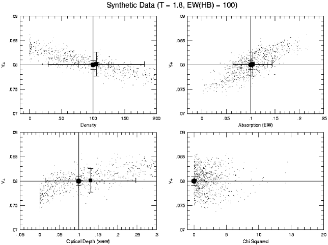
Figure 5: Similar plot to Figure 4 except that the underlying absorption is 0.1 Å and $\tau$(3889) $=$ 0.1.

Figure 5 shows the results of the Monte Carlo when both $\tau$ and $a_{HeI}\neq 0$, and $n=100$ cm^-3. It is encouraging that in perhaps more realistic cases where the input parameters are non-zero, we are able to derive results very close to their correct values. The average of Monte Carlo realizations is remarkably close to the straight minimization for all of the derived parameters ($n,a_{HeI},\tau$ and $y^{+}$). However, there is an enormous dispersion in these results due to the degeneracy in the solutions with respect to the physical input parameters. This results in error estimates for parameters which are significantly larger than in the straight minimization. For example, the uncertainties in both the density and optical depth are almost a factor of 3 times larger in the Monte Carlo. When propagated into the uncertainty in the derived value for the He abundance, we find that the uncertainty in the Monte Carlo result (which we argue is a better, not merely more conservative, value) is a factor of 2.5 times the uncertainty obtained from a straight minimization using 6 line He lines. This amounts to an approximately 4% uncertainty in the He abundance, despite the fact that we assumed (in the synthetic data) 2% uncertainties in the input line strengths. This is an unavoidable consequence of the method - the Monte Carlo routine explores the degeneracies of the solutions and reveals the larger errors that should be associated with the solutions.

In Figure 6, I show the result of a single case based on the data of ref. it for SBS1159+545. Here, the helium abundance and density solutions are displayed. The vertical and horizontal lines show the position of the solution in it . The circle shows the position of the our solution to the minimization, and the square shows the position of the mean of the Monte-Carlo distribution. The spread shown here is significantly greater than the uncertainty quoted in it .

Figure 6: A Monte Carlo determination of the helium abundance and electron density (in cm^-3) for the region SBS11159+545. Solutions for $a^{\prime}$ and $\tau$ are not shown here.

2.2 ⁷Li

The abundance of ⁷Li has been determined by observations of over 100 hot, population-II halo stars, and is found to have a very nearly uniform abundancesp . For stars with a surface temperature $T>5500$ K and a metallicity less than about 1/20th solar (so that effects such as stellar convection may not be important), the abundances show little or no dispersion beyond that which is consistent with the errors of individual measurements. The Li data from Ref.mol indicate a mean ⁷Li abundance of

$${\rm Li/H=(1.6\pm 0.1)\times 10^{-10}}$$ (7)

The small error is statistical and is due to the large number of stars in which ⁷Li has been observed. The solid box for ⁷Li in Figure 1 represents the 2$\sigma_{\rm stat}$ range from (7).

There is, however, an important source of systematic error due to the possibility that Li has been depleted in these stars, though the lack of dispersion in the Li data limits the amount of depletion. In fact, a small observed slope in Li vs Fe and the tiny dispersion about that correlation indicates that depletion is negligible in these stars rnb . Furthermore, the slope may indicate a lower abundance of Li than that in (6). The observationli6o of the fragile isotope ⁶Li is another good indication that ⁷Li has not been destroyed in these starsli6 .

The weighted mean of the ⁷Li abundance in the sample of ref. rnb is [Li] = 2.12 ([Li] = $\log$ ⁷Li/H + 12) and is slightly lower than that in eq. (7), the difference is a systematic effect due to analysis methods. It is common to test for the presence of a slope in the Li data by fitting a regression of the form [Li] = $\alpha+\beta$ [Fe/H]. These data indicate a rather large slope, $\beta=0.07-0.16$ and hence a downward shift in the “primordial” lithium abundance $\Delta$[Li] = $-0.20--0.09$. Models of galactic evolution which predict a small slope for [Li] vs. [Fe/H], can produce a value for $\beta$ in the range 0.04 – 0.07 rbofn . Of course, if we would like to extract the primordial ⁷Li abundance, we must examine the linear (rather than log) regressions. For Li/H = $a^{\prime}+b^{\prime}$Fe/Fe_⊙, we find $a^{\prime}=1-1.2\times 10^{-10}$ and $b^{\prime}=40-120\times 10^{-10}$. A similar result is found fitting Li vs O. Overall, when the regression based on the data and other systematic effects are taken into account a best value for Li/H was found to be rbofn

$${\rm Li/H=1.23\times 10^{-10}}$$ (8)

with a plausible range between 0.9 – 1.9 $\times 10^{-10}$. The dashed box in Figure 1 corresponds to this range in Li/H.

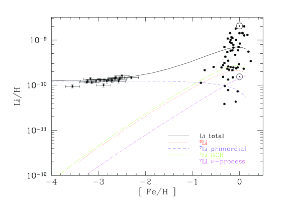
Figure 7: Contributions to the total predicted lithium abundance from the adopted GCE model of ref. fo98 , compared with low metallicity stars (from rnb ) and a sample of high metallicity stars. The solid curve is the sum of all components.

Figure 7 shows the different Li components for a model with (⁷Li/H)${}_{p}=1.23\times 10^{-10}$. The linear slope produced by the model is $b^{\prime}=65\times 10^{-10}$, and is independent of the input primordial value (unlike the log slope given above). The model fo98 includes in addition to primordial ⁷Li, lithium produced in galactic cosmic ray nucleosynthesis (primarily $\alpha+\alpha$ fusion), and ⁷Li produced by the $\nu$-process during type II supernovae. As one can see, these processes are not sufficient to reproduce the population I abundance of ⁷Li, and additional production sources are needed.

3 LiBeB

The question that one should ask with regard to the above discussion of ⁷Li (and as we will see below when discussing concordance, ⁷Li will play an important role in determining the baryon density $\eta$), is whether or not there is additional evidence for the post big bang production of ⁷Li. There is in fact evidence in the related observation of the intermediate mass elements of ⁶Li, Be and B. While these elements are produced in the big bang tsof , their predicted primordial abundance is far below their observed abundance, which like ⁷Li is determined by observations of old metal poor halo stars. Whereas in the range $\eta_{10}=1.5-4.5$, standard BBN predicts abundances of

$$\hbox{${}^{6}$Li}/{\rm H} \approx (2-9)\times 10^{-14}$$ (9)

$$\hbox{${}^{9}$Be}/{\rm H} \approx (0.04-2)\times 10^{-17}$$ (10)

$$\hbox{${}^{10}$B}/{\rm H} \approx (0.5-3)\times 10^{-19}$$ (11)

$$\hbox{${}^{11}$B}/{\rm H} \approx (0.02-1)\times 10^{-16}$$ (12)

the observed abundances found in Pop II halo stars are: ⁶Li/H $\approx$ few $\times~{}10^{-12}$, ⁹Be/H $\sim 1-10\times 10^{-13}$, and B/H $\sim 1-10\times 10^{-12}$. It is generally recognized that these isotopes are not of primordial origin, but rather have been produced in the Galaxy, through cosmic-ray nucleosynthesis.

Be and B have been observed in the same pop II stars which show Li and in particular there are a dozen or so stars in which both Be and ⁷Li have been observed. Thus Be (and B though there is still a paucity of data) can be used as a consistency check on primordial Li. Based on the Be abundance found in these stars, one can conclude that no more than 10-20% of the ⁷Li is due to cosmic ray nucleosynthesis leaving the remainder (the abundance in Eq. (8)) as primordial. This is consistent with the conclusion reached in Ref.rbofn .

In principle, we can use the abundance information on the other LiBeB isotopes to determine the abundance of the associated GCRN produced ⁷Li. As it turns out, the boron data is problematic for this purpose, as there is very likely an additional significant source for ¹¹B, namely $\nu$-process nucleosynthesis in supernovae. Using the subset of the data for which Li and Be have been observed in the same stars, one can extract the primordial abundance of ⁷Li in the context of a given model of GCRN. For example, a specific GCRN model, predicts the ratio of Li/Be as a function of [Fe/H]. Under the (plausible) assumption that all of the observed Be is GCRN produced, the Li/Be ratio would yield the GCRN produced ⁷Li and could then be subtracted from each star to give a set of primordial ⁷Li abundances. This was done in os where it was found that the plateau was indeed lowered by approximately 0.07 dex. However, it should be noted that this procedure is extremely model dependent. The predicted Li/Be ratio in GCRN models was studied extensively in fos . It was found that Li/Be can vary between 10 and $\sim 300$ depending on the details of the cosmic-ray sources and propagation–e.g., source spectra shapes, escape pathlength magnitude and energy dependence, and kinematics.

In contrast, the ⁷Li/⁶Li ratio is much better determined and far less model dependent since both are predominantly produced by $\alpha-\alpha$ fusion rather than by spallation. The obvious problem however, is the paucity of ⁶Li data. As more ⁶Li data becomes available, it should be possible to obtain a better understanding of the relative contribution to ⁷Li from BBN and GCRN.

The associated BeB elements are clearly of importance in determining the primordial ⁷Li abundance, since Li is produced together with Be and B in accelerated particle interactions such as cosmic ray spallation. However, these production processes are not yet fully understood. Standard cosmic-ray nucleosynthesis is dominated by interactions originating from accelerated protons and $\alpha$’s on CNO in the ISM, and predicts that BeB should be “secondary” versus the spallation targets, giving $\hbox{$$Be}\propto{\rm O}^{2}$. However, this simple model was challenged by the observations of BeB abundances in Pop II stars, and particularly the BeB trends versus metallicity. Measurements showed that both Be and B vary roughly linearly with Fe, a so-called “primary” scaling. If O and Fe are co-produced (i.e., if O/Fe is constant at low metallicity) then the data clearly contradicts the canonical theory, i.e. BeB production via standard GCR’s.

There is growing evidence that the O/Fe ratio is not constant at low metallicityisr , but rather increases towards low metallicity. This trend offers a solution to resolve discrepancy between the observed BeB abundances as a function of metallicity and the predicted secondary trend of GCR spallation fo98 . As noted above, standard GCR nucleosynthesis predicts $\hbox{$$Be}\propto{\rm O}^{2}$, while observations show $\hbox{$$Be}\sim{\rm Fe}$, roughly; these two trends can be consistent if O/Fe is not constant in Pop II. A combination of standard GCR nucleosynthesis, and $\nu$-process production of ¹¹B may be consistent with current data.

Thus the nature of the production mechanism for BeB (primary vs. secondary) rests with the determination of ratio of O/Fe at low metallicity. In any case, it is clear that given a primary mechanism, it will be dominant in the early phases of the Galaxy, and secondary mechanisms will dominate in the latter stage of galactic evolution. The cross over or break point is uncertain. In Figure 8, a plausible model for the evolution of BeB is shown and compared with the data fovc . Shown by the short dashed lines are standard galactic cosmic-ray nucleosynthesis, which is mostly secondary, but contains some primary production as well. The long dashed curves are purely primary, and in the case of boron, the $\nu$ process has been included and this too is primary. The solid curves represent the total Be and B abundance as a function of [O/H]. As one can see such a model fits the data quite well.

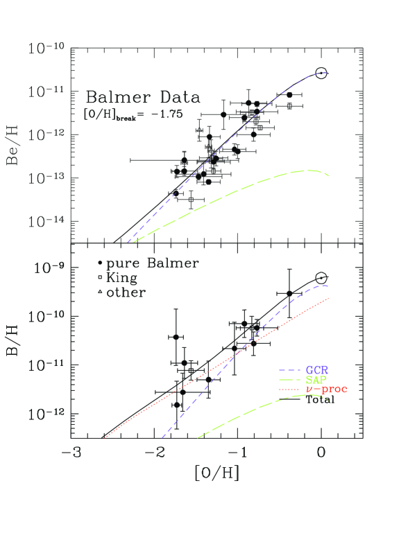
Figure 8: Be vs O (top panel) and B vs O (bottom panel). Data shown are found to have a break point as indicated. Models are adjusted to achieve the break point and O/Fe slope of these data.

4 Concordance

Let us now to turn to the question of concordance between the BBN predictions and the observations discussed above. This is best summarized in a comparison of likelihood functions as a function of the one free parameter of BBN, namely the baryon-to-photon ratio $\eta$. By combining the theoretical predictions (and their uncertainties) with the observationally determined abundances discussed above, we can produce individual likelihood functions fo which are shown in Figure 9. A range of primordial ⁷Li values are chosen based on the the abundances in Eqs. (7) and (8) as well as a higher and lower value. The double peaked nature of the ⁷Li likelihood functions is due to the presence of a minimum in the predicted lithium abundance in the expected range for $\eta$. For a given observed value of ⁷Li, there are two likely values of $\eta$. As the lithium abundance is lowered, one tends toward the minimum of the BBN prediction, and the two peaks merge. Also shown are both values of the primordial ⁴He abundances discussed above. As one can see, at this level there is clearly concordance between ⁴He, ⁷Li and BBN.

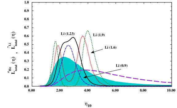
Figure 9: Likelihood distributions for four values of primordial ⁷Li/H ($10^{10}\times$ ⁷Li = 1.9 (dashed), 1.6 (dotted), 1.23 (solid), and 0.9 (dash-dotted)), and for ⁴He (shaded) for which we adopt $Y_{p}=0.238\pm 0.002\pm 0.005$ (Eq. (1)). Also shown by the long dashed curve is the likelihood function based on the ⁴He abundance from Eq. (2).

The combined likelihood, for fitting both elements simultaneously, is given by the product of two of the functions in Figure 9. The combined likelihood is shown in Figure 10, for the two primordial values of ⁷Li in Eqs. (7) and (8). For ⁷Li${}_{p}=1.6\times 10^{-10}$ (shown as the dashed curve), the 95% CL region covers the range $1.55<\eta_{10}<4.45$, with the two peaks occurring at $\eta_{10}=1.9$ and 3.5. This range corresponds to values of $\Omega_{B}$ between

$$0.006<\Omega_{B}h^{2}<.016$$ (13)

For ⁷Li${}_{p}=1.23\times 10^{-10}$ (shown as the solid curve), the 95% CL region covers the range $1.75<\eta_{10}<3.90$. In this case, the primordial value is low enough that the two lithium peaks are more or less merged as is the total likelihood function giving one broad peak centered at $\eta_{10}\simeq 2.5$. The corresponding values of $\Omega_{B}$ in this case are between

$$0.006<\Omega_{B}h^{2}<.014$$ (14)

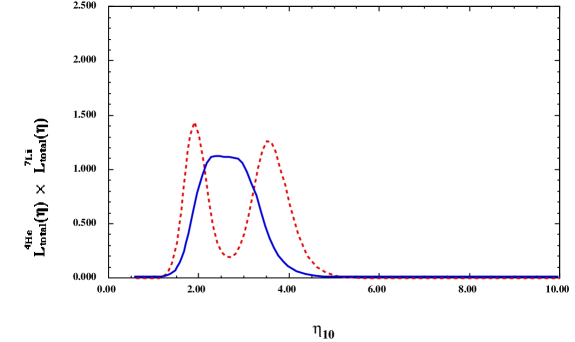
Figure 10: Combined likelihood distributions for two values of primordial ⁷Li/H ($10^{10}\times$ ⁷Li = 1.6 (dashed), 1.23 (solid)), and ⁴He with $Y_{p}=0.238\pm 0.002\pm 0.005$ (Eq. (1)).

When deuterium is folded into the mix, the situation becomes more complicated. Although there are several good measurements of deuterium in quasar absorption systems burles , and many of them giving a low value of D/H $\simeq(3.4\pm 0.3)\times 10^{-5}$ bty , there remains an observation with D/H nearly an order of magnitude higher D/H $\simeq(2.0\pm 0.5)\times 10^{-4}$ webb .

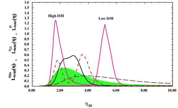
Figure 11: Likelihood distributions for two values of primordial ⁷Li/H ($10^{10}\times$ ⁷Li = 1.6 (dashed) and 1.23 (solid)), and ⁴He with $Y_{p}=0.238\pm 0.002\pm 0.005$ from Eq. (1) (shaded) and $Y_{p}=0.244\pm 0.002\pm 0.005$ from Eq. (2) (long dashed). Also shown are the two likelihood functions for high and low D/H as marked.

Because there are no known astrophysical sites for the production of deuterium, all observed D is assumed to be primordial. As a result, any firm determination of a deuterium abundance establishes an upper bound on $\eta$ which is robust. Thus the ISM measurementslin of D/H = 1.6 $\times 10^{-5}$ imply an upper bound $\eta_{10}<9$.

It is interesting to compare the results from the likelihood functions of ⁴He and ⁷Li with that of D/H. This comparison is shown in Figure 11. Using the higher value of D/H = $(2.0\pm 0.5)\times 10^{-4}$, we would find excellent agreement between ⁴He, ⁷Li and D/H. The predicted range for $\eta$ now becomes

$$1.6<\eta_{10}<3.2$$ (15)

with the peak likelihood value at $\eta_{10}=2.1$, ⁴He and ⁷Li abundances from eqs. (1) and (8) respectively. This corresponds to $\Omega_{B}h^{2}=.008^{+.004}_{-.002}$. The higher ⁷Li abundance of eq. (7) drops the peak value down slightly to $\eta_{10}=1.8$ and broadens the range to 1.5 – 3.4. The higher ⁴He abundance shifts the peak and range (relative to eq. (15)) up to 2.2 and 1.7 – 3.5.

Figure 12: 50%, 68% & 95% C.L. contours of $L_{47}$ and $L_{247}$ where observed abundances are given by eqs. (1 and 7), and high D/H.

If instead, we assume that the low value of D/H = $(3.4\pm 0.3)\times 10^{-5}$ bty is the primordial abundance, there is hardly any overlap between the D and ⁷Li, particularly for the lower value of ⁷Li from eq. (8). There is also very limited overlap between D/H and ⁴He, though because of the flatness of the ⁴He abundance with respect to $\eta$, as one can see, the likelihood function for the larger value of ⁴He from eq. (2) is very broad. In this case, D/H is just compatible (at the 2 $\sigma$ level) with the other light elements, and the peak of the likelihood function occurs at roughly $\eta_{10}=4.8$ and with a range of 4.2 – 5.6.

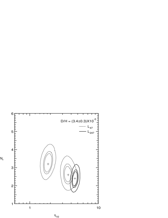
Figure 13: 50%, 68% & 95% C.L. contours of $L_{47}$ and $L_{247}$ where observed abundances are given by eqs. (1 and 7), and low D/H.

It is important to recall however, that the true uncertainty in the low D/H systems might be somewhat larger. Mesoturbulence effectslev allow D/H to be as large as $5\times 10^{-5}$. In this case, the peak of the D/H likelihood function shifts down to $\eta_{10}\simeq 4$, and there would be a near perfect overlap with the high $\eta$ ⁷Li peak and since the ⁴He distribution function is very broad, this would be a highly compatible solution.

We can obtain still more information regarding the compatibility of the observed abundance and BBN by considering generalized likelihood functions where we allow $N_{\nu}$ to vary as well fo ; oth2 ; oth3 ; sark2 . The likelihood functions now become functions of two parameters ${\cal L}(\eta,N_{\nu})$.

The peaks of the distribution as well as the allowed ranges of $\eta$ and $N_{\nu}$ are easily discerned in the contour plots of Figures 12 and 13 which show the 50%, 68% and 95% confidence level contours in $L_{47}$ and $L_{247}$ projected onto the $\eta$–$N_{\nu}$ plane, for high and low D/H as indicated. $L_{47}$ corresponds to the likelihood function based on ⁴He and ⁷Li only, whereas $L_{247}$ includes D/H as well. The crosses show the location of the peaks of the likelihood functions. $L_{47}$ peaks at $N_{\nu}=3.2$, $\eta_{10}=1.85$ and at $N_{\nu}=2.6$, $\eta_{10}=3.6$. The 95% confidence level allows the following ranges in $\eta$ and $N_{\nu}$

$$1.7\leq N_{\nu}\leq 4.3\qquad\qquad 1.4\leq\eta_{10}\leq 4.9$$ (16)

Note however that the ranges in $\eta$ and $N_{\nu}$ are strongly correlated as is evident in Figure 12.

With high D/H, $L_{247}$ peaks at $N_{\nu}=3.3$, and also at $\eta_{10}=1.85$. In this case the 95% contour gives the ranges

$$2.2\leq N_{\nu}\leq 4.4\qquad\qquad 1.4\leq\eta_{10}\leq 2.4$$ (17)

Note that within the 95% CL range, there is also a small area with $\eta_{10}=3.2-3.5$ and $N_{\nu}=2.5-2.9$.

Similarly, for low D/H, $L_{247}$ peaks at $N_{\nu}=2.4$, and $\eta_{10}=4.55$. The 95% CL upper limit is now $N_{\nu}<3.2$, and the range for $\eta$ is $3.9<\eta_{10}<5.4$. It is important to stress that these abundances are now consistent with the standard model value of $N_{\nu}=3$ at the 2 $\sigma$ level.

References

-
(1)
T.P. Walker, G. Steigman, D.N. Schramm,
K.A. Olive and K. Kang, Ap.J. 376 (1991)
51;
S. Sarkar, Rep. Prog. Phys. 59 (1996) 1493;
K.A. Olive, astro-ph/9901231; K.A. Olive, G. Steigman, and T.P. Walker, Phys. Rep. 333-334 (2000) 389. -
(2)
L.M. Krauss and P. Romanelli, Ap.J. 358 (1990) 47;
M. Smith, L. Kawano, and R.A. Malaney, Ap.J. Supp. 85 (1993) 219. - (3) N. Hata, R.J. Scherrer, G. Steigman, D. Thomas, and T.P. Walker, Ap.J. 458 (1996) 637.
- (4) G. Fiorentini, E. Lisi, S. Sarkar, and F.L. Villante, Phys.Rev. D58 (1998) 063506.
- (5) K. M. Nollett and S. Burles, Phys. Rev. D61 (2000) 123505.
- (6) D.E. Groom et al. Eur. Phys. J. C15 (2000) 1.
-
(7)
B.D. Fields and K.A. Olive, Phys. Lett. B368
(1996) 103;
B.D. Fields, K. Kainulainen, D. Thomas, and K.A. Olive, New Ast. 1 (1996) 77. -
(8)
B.E.J. Pagel, E.A. Simonson, R.J. Terlevich and M. Edmunds,
MNRAS 255 (1992) 325;
E. Skillman and R.C. Kennicutt, Ap.J. 411 (1993) 655;
E. Skillman, R.J. Terlevich, R.C. Kennicutt, D.R. Garnett, and E. Terlevich, Ap.J. 431 (1994) 172. - (9) Y.I. Izotov, T.X. Thuan, and V.A. Lipovetsky, Ap.J. 435 (1994) 647; Ap.J.S. 108 (1997) 1.
- (10) Y.I. Izotov, and T.X. Thuan, Ap.J. 500 (1998) 188.
-
(11)
K.A. Olive, E. Skillman, and G. Steigman, Ap.J.
483 (1997) 788;
B.D. Fields and K.A. Olive, Ap.J. 506 (1998) 177. - (12) M. Peimbert, A. Peimbert, and M.T. Ruiz, astro-ph/0003154.
- (13) K.A. Olive and E. Skillman, astro-ph/0007081.
- (14) F. Spite, and M. Spite, A.A. 115 (1982) 357.
-
(15)
P. Molaro, F. Primas, and P. Bonifacio, A.A. 295
(1995) L47;
P. Bonifacio and P. Molaro, MNRAS 285 (1997) 847. - (16) S.G. Ryan, J.E. Norris, and T.C. Beers, Ap.J. 523 (1999) 654.
-
(17)
V.V. Smith, D.L. Lambert, and P.E. Nissen, Ap.J. 408
(1992) 262; Ap.J. 506
(1998) 405;
L. Hobbs, and J. Thorburn, Ap.J. 428 (1994) L25; Ap.J. 491 (1997) 772;
R. Cayrel, M. Spite, F. Spite, E. Vangioni-Flam, M. Cassé, and J. Audouze, A.A. 343 (1999) 923. -
(18)
G. Steigman, B. Fields, K.A. Olive, D.N. Schramm, and
T.P. Walker, Ap.J. 415 (1993) L35;
M. Lemoine, D.N. Schramm, J.W. Truran, and C.J. Copi, Ap.J. 478 (1997) 554;
M.H. Pinsonneault, T.P. Walker, G. Steigman, and V.K. Naranyanan, Ap.J. 527, 180 (1998);
B.D.Fields and K.A. Olive, New Astronomy, 4 (1999) 255;
E. Vangioni-Flam, M. Cassé, R. Cayrel, J. Audouze, M. Spite, and F. Spite, New Astronomy, 4 (1999) 245. - (19) S.G. Ryan, T.C. Beers, K.A. Olive, B.D. Fields, and J.E. Norris, Ap.J. Lett. 530 (2000) L57.
- (20) B. Fields and K.A. Olive, Ap.J. 506, 177 (1998).
- (21) D. Thomas, D.N. Schramm, K.A. Olive, and B.D. Fields, Ap.J. 406 (1993) 569.
- (22) K.A. Olive, and D.N. Schramm, Nature 360 (1993) 439.
- (23) B.D. Fields, K.A. Olive, and D.N. Schramm, Ap.J. 435 (1994) 185.
-
(24)
G. Israelian, R.J. García-López, and R. Rebolo,
Ap.J. 507, 805 (1998);
A.M. Boesgaard, J.R. King, C.P. Deliyannis, and S.S. Vogt, A.J. 117, 492 (1999). - (25) B.D. Fields, K.A. Olive, E. Vangioni-Flam, and M. Cassé, Ap.J. 540 (2000) 930.
- (26) S. Burles, these proceedings.
- (27) S. Burles and D. Tytler, Ap.J. 499 (1998) 699; Ap.J. 507 (1998) 732.
-
(28)
J.K. Webb, R.F. Carswell, K.M. Lanzetta, R. Ferlet, M.
Lemoine, A. Vidal-Madjar, and D.V. Bowen, Nature 388 (1997)
250;
D. Tytler, S. Burles, L. Lu, X.-M. Fan, A. Wolfe, and B.D. Savage, A.J. 117 (1999) 63. - (29) J.L. Linsky, et al., Ap.J. 402 (1993) 694; J.L. Linsky, et al.,Ap.J. 451 (1995) 335.
- (30) S. Levshakov, D. Tytler, and S. Burles, astro-ph/9812114.
- (31) K.A. Olive and D. Thomas, Astro. Part. Phys. 7 (1997) 27.
- (32) K.A. Olive and D. Thomas, Astro. Part. Phys. 11 (1999) 403.