Gamma-Ray Bursts from Up-Scattered Self-Absorbed Synchrotron Emission

Abstract

We calculate the synchrotron self-Compton emission from internal shocks occurring in relativistic winds as a source of gamma-ray bursts, with allowance for self-absorption. For plausible model parameters most pulses within a Gamma-Ray Burst (GRB) are optically thick to synchrotron self-absorption at the frequency at which most electrons radiate. Up-scattering of photon number spectra harder than $\nu^{0}$ (such as the self-absorbed emission) yields inverse Compton photon number spectra that are flat, therefore our model has the potential of explaining the low-energy indices harder than $\nu^{-2/3}$ (the optically thin synchrotron limit) that have been observed in some bursts. The optical counterparts of the model bursts are sufficiently bright to be detected by such experiments as LOTIS, unless the magnetic field is well below equipartition.

Dept. of Astrophysical Sciences, Princeton University, Princeton, NJ 08544

and Institute for Advanced Study, Olden Lane, Princeton, NJ 08540,
Institute of Astronomy, Madingley Road, Cambridge CB3 0HA, U.K.,
Dept. of Astronomy & Astrophysics, Pennsylvania State University, University Park, PA 16802

Subject headings: gamma-rays: bursts - methods: numerical - radiation mechanisms: non-thermal

1 Introduction

In the framework of internal shocks occurring in highly relativistic winds, the up-scattering of synchrotron photons was taken into consideration in the calculation GRB spectra by Papathanassiou & Mészáros (1996) and Pilla & Loeb (1998). Both groups found a reasonable qualitative agreement between modeled and observed spectra. As shown in §2.2, for electron injection fractions of order unity and reasonable dissipation efficiencies, synchrotron emission is liable to peak below the spectral peak observed in GRBs at hundreds of keVs (Band et al. 1993), even for equipartition magnetic fields. For this reason we consider a GRB model where the synchrotron peak is in/around the optical range, and the $\gamma$-photons arise from inverse Compton (IC) scatterings (Mészáros & Rees 1994). In this case synchrotron self-absorption (SSA) can be important at the synchrotron peak, yielding up-scattered spectra that are harder below 100 keV than an optically thin synchrotron emission peaking at hard $X$-rays.

In this work we obtain numerically the synchrotron self-Compton emission from internal shocks through simulations of the wind dynamical evolution and the emission released in each collision. We also investigate the brightness of the optical flashes radiated by internal shocks (Mészáros & Rees 1997). IC scattering of synchrotron seed photons has been previously considered as a mechanism of emission of high energy photons in GRB afterglows (e.g. Mészáros & Rees 1994, Sari, Narayan, & Piran 1996, Waxman 1997, Chiang & Dermer 1999, Panaitescu & Kumar 2000) and in blazars (e.g. Boettcher, Mause, & Schlickeiser 1997, Mastichiadis & Kirk 1997, Urry 1998, Chiaberge & Ghisellini 1999).

2 Description of the Model

2.1 Wind Dynamics

The relativistic wind is approximated as a sequence of discrete shells of uniform density, ejected by the GRB source with various initial Lorentz factors and masses. We assume that the time it takes the GRB engine to become unstable and eject a shell is proportional to the energy of that shell. This implies a constant wind luminosity $L$ on average throughout the entire wind ejection duration $t_{w}$. We consider that the shell Lorentz factors $\Gamma$ have a log-normal distribution (Beloborodov 2000), $\Gamma-1=(\Gamma_{0}-1)\exp(Ax)$ with $x$ Gaussian distributed, and $A$ of order unity.

The radii at which the collisions between pairs of neighboring shells take place are calculated from the ejection kinematics, taking into account the progressive merging, the adiabatic losses between collisions, and the radiative losses. The Lorentz factor and internal energy of the shocked fluid are calculated from energy and momentum conservation in each shell collision. The shock jump conditions (Blandford & McKee 1976) determine the speeds of each shock, which give: $i)$ the shocked fluid energy density $u^{\prime}$ (used for calculating the magnetic field $B$ and minimum electron Lorentz factor $\gamma_{i}$, see §2.2); $ii)$ the shell shock-crossing time $t^{\prime}_{i}$ (which is the duration of the injection of electrons, determining the cooling electron Lorentz factor $\gamma_{c}$, see §2.3); and $iii)$ the post-shock shell thickness $\Delta^{\prime}$ (used for calculating the adiabatic cooling timescale and the radiative efficiency). Between collisions the co-moving frame thickness increases at the sound speed.

2.2 Emission of Radiation

The synchrotron self-Compton emission from each shocked shell is calculated from the Lorentz factor, magnetic field, number of electrons (given by the shell mass) and the electron distribution in each shocked shell. The turbulent magnetic field strength $B$ and the typical electron Lorentz factor $\gamma_{i}$ resulting from shock-acceleration are parameterized through their fractional energy $\xi$ and $\varepsilon$ relative to the internal energy:

$$B^{2}=8\pi\,\xi\,u^{\prime}\quad,\quad\gamma_{i}=\frac{p-2}{p-1}\frac{\varepsilon\,u^{\prime}}{n^{\prime}_{e}\,m_{e}c^{2}}\;,$$ (1)

where $u^{\prime}$ and $n^{\prime}_{e}$ are the internal energy and particle density, respectively, and $p$ is the index of the power-law distribution of injected electrons: ${\cal N}_{i}(\gamma)\propto\gamma^{-p}$ for $\gamma\geq\gamma_{i}$. Denoting by $\theta$ the laboratory frame internal-to-kinetic energy ratio in the shocked fluid (i.e. the dissipation efficiency), one can write $u^{\prime}\simeq\theta\,n^{\prime}_{e}m_{p}c^{2}$, hence

$$\gamma_{i}=({m_{p}}/{2\,m_{e}})\;\varepsilon\,\theta=30\;\varepsilon_{-.5}\,\theta_{-1}\;,$$ (2)

with $A_{n}\equiv 10^{-n}A$ and using $p=3$ for simplicity.

The density $n^{\prime}_{e}$ can be calculated from the shell mass $m$, thickness $\Delta^{\prime}$, and radius $r$, using $m=4\pi r^{2}m_{p}n^{\prime}_{e}\Delta^{\prime}$. For analytical calculations one can approximate the typical mass $m$ of a shell radiating a pulse which arrives at observer time $T$ as a fraction $T/T_{b}$ of the total wind mass $M$, where $T_{b}$ is the burst duration, which is approximately equal to the duration $t_{w}$ of the wind ejection. One obtains $m=LT/\Gamma c^{2}$, where $L\equiv E/t_{w}$ is the wind luminosity, $E$ and $\Gamma$ being the wind total energy average Lorentz factor of the wind. The collisional radius $r$ can be derived from the spread in the photon arrival time $\delta=r/\Gamma^{2}c$ due to the spherical shape of the emitting surface, which is roughly the pulse duration. The shell thickness can be approximated by $\Delta^{\prime}=r/\Gamma$. Therefore we obtain $n^{\prime}_{e}=LT/(4\pi m_{p}c^{5}\Gamma^{6}\delta^{3})$. Then equation (1) yields

$$B=\frac{\left(2\,\xi\theta LT\right)^{1/2}}{\Gamma^{3}(c\delta)^{3/2}}=3\times 10^{4}\;\xi_{-1}^{1/2}\,\theta_{-1}^{1/2}\,L_{53}^{1/2}\,\Gamma_{2}^{-3}\,\delta_{0}^{-3/2}T_{1}^{1/2}\;{\rm(G)}\;.$$ (3)

If the emission at $\nu_{i}$ is not self-absorbed, then the peak frequency $\nu_{sy}$ of the synchrotron power $\nu F_{\nu}^{(sy)}$ is at the characteristic synchrotron frequency $\nu_{i}=(eB\gamma_{i}^{2}\Gamma)/(4\,m_{e}c)$ of the $\gamma_{i}$-electrons, and the peak of the IC power $\nu F_{\nu}^{(ic)}$ is at $\nu_{ic}\simeq\gamma_{i}^{2}\nu_{i}$. From equations (2) and (3), one obtains that

$$\nu_{sy}=10^{16}\,\varepsilon_{-.5}^{2}\xi_{-1}^{1/2}\theta_{-1}^{5/2}L_{53}^{1/2}\Gamma_{2}^{-2}\,\delta_{0}^{-3/2}T_{1}^{1/2}\;{\rm(Hz)}\;,$$ (4)

$$\nu_{ic}\simeq 10^{19}\,\varepsilon_{-.5}^{4}\xi_{-1}^{1/2}\theta_{-1}^{9/2}L_{53}^{1/2}\Gamma_{2}^{-2}\,\delta_{0}^{-3/2}T_{1}^{1/2}\;{\rm(Hz)}\;.$$ (5)

Equations (4) and (5) show that the peak frequencies of the optically thin synchrotron and of the IC emissions depend strongly on parameters which may vary substantially from pulse to pulse. Equation (4) also shows that for plausible model parameters the synchrotron peak $h\nu_{sy}$ cannot be as high as 100 keV for pulses longer than about $\delta=0.1\,{\rm s}$.

Due to the collisions among shells, the amplitude of the Lorentz factor fluctuations in the wind is reduced, diminishing the dissipation efficiency $\theta$. Equation (5) shows that the peak of the IC emission depends strongly on $\theta$ and thus should have a general trend of decreasing in time. This could be the reason for the overall spectral softening seen in GRBs (e.g. Ford et al. 1995).

2.3 Electron Distribution

The electron distribution ${\cal N}(\gamma)$ at the end of shell energization is determined by the ${\cal N}_{i}(\gamma)$ initially injected at shock, by the electron radiative cooling (through synchrotron and IC radiation) and by the absorption of the synchrotron photons. The radiative cooling timescale of electrons with Lorentz factor $\gamma$ is $t^{\prime}_{r}(\gamma)\sim(\gamma m_{e}c^{2})/(P^{\prime}_{sy}+P^{\prime}_{ic})$, where $P^{\prime}_{ic}=YP^{\prime}_{sy}$ is the electron IC radiating power and $P^{\prime}_{sy}=(1/6\pi)\sigma_{Th}c\gamma^{2}B^{2}$ is the synchrotron power, thus

$$t^{\prime}_{r}(\gamma)=\frac{C_{1}}{(Y+1)\gamma}t^{\prime}_{i}\;,\quad C_{1}\equiv\frac{6\pi m_{e}c}{\sigma_{Th}B^{2}t^{\prime}_{i}}\;,$$ (6)

$t^{\prime}_{i}$ being the time elapsed since the beginning of injection of relativistic electrons, i.e. the shell shock-crossing time, which is calculated numerically from the shock dynamics.

From equation (6) the cooling electron Lorentz factor $\gamma_{c}$ defined by $t^{\prime}_{r}(\gamma_{c})=t^{\prime}_{i}$ is $\gamma_{c}=C_{1}/(Y+1)$. For $\gamma_{c}<\gamma_{i}$ the $\gamma_{i}$-electrons cool faster than their injection timescale. In this fast electron cooling regime the resulting electron distribution has a low-energy tail ${\cal N}(\gamma)\propto\gamma^{-2}$ for $\gamma_{c}<\gamma<\gamma_{i}$, while ${\cal N}(\gamma)\propto\gamma^{-(p+1)}$ above $\gamma_{i}$. In the slow electron cooling regime, characterized by $\gamma_{i}<\gamma_{c}$, the electron distribution is the injected one, ${\cal N}(\gamma)\propto\gamma^{-p}$, for $\gamma_{i}<\gamma<\gamma_{c}$, and ${\cal N}(\gamma)\propto\gamma^{-(p+1)}$ above $\gamma_{c}$, due to cooling. As physical parameters vary among shocked shells, the GRB pulses can be in different electron cooling regimes.

2.4 Compton Parameter and Self-Absorption Break

We set the electron distribution as described in §2.3. The Compton parameter is given by

$$Y=\tau_{e}\left[\int_{0}^{\gamma_{a}}{\cal N}(\gamma)\frac{\gamma^{2}}{\tau_{a}(\gamma)}{\rm d}\gamma+\int_{\gamma_{a}}^{\infty}{\cal N}(\gamma)\gamma^{2}{\rm d}\gamma\right]\;,$$ (7)

where $\tau_{e}$ is the optical depth to electron scattering and $\tau_{a}(\gamma)$ is the optical thickness to SSA at the synchrotron characteristic frequency for $\gamma$-electrons, and $\gamma_{a}$ is defined by $\tau_{a}(\gamma_{a})=1$. The first integral in the right-hand side of equation (7) takes into account that only those photons emitted within a region (around a given electron) of optical depth unity are up-scattered before being absorbed. Table 1 lists the values of the Y parameter for all possible orderings of $\gamma_{a}$, $\gamma_{c}$, and $\gamma_{i}$, assuming that these breaks are sufficiently apart from each other, and ignoring multiplicative factors of order unity.

For a power-law distribution of electrons it can be shown that the optical thickness $\tau_{a}$ to SSA at the characteristic synchrotron frequency for electrons at the top of the distribution, i.e. at $\gamma_{p}=\min(\gamma_{c},\gamma_{i})$, is

$$\tau_{p}\simeq\frac{C_{2}}{\gamma_{p}^{5}}\;,\quad C_{2}\equiv\frac{5\,e\tau_{e}}{\sigma_{Th}B}\;.$$ (8)

For slow electron cooling ($\gamma_{p}=\gamma_{i}$) one obtains

$$\tau_{p}=3\times 10^{4}\;\varepsilon_{-.5}^{-5}\xi_{-1}^{-1/2}\theta_{-1}^{-11/2}L_{53}^{1/2}\Gamma_{2}^{-2}\delta_{0}^{-1/2}T_{1}^{1/2}\;.$$ (9)

If electrons are cooling fast ($\gamma_{p}=\gamma_{c}$), then $\tau_{p}$ is even larger. Equation (9) shows that is quite likely that the synchrotron emission from the typical, $\gamma_{p}$-electron is self-absorbed, thus the synchrotron spectrum $F_{\nu}$ peaks at the synchrotron frequency $\nu_{a}$ corresponding to $\gamma_{a}$.

The shell optical thickness to SSA at any frequency $\nu$ (or corresponding $\gamma$) can be calculated from $\tau_{p}$ given in equation (8) by using $\tau_{a}(\nu)\propto\nu^{-5/3}\propto\gamma^{-10/3}$ for $\gamma<\gamma_{p}$ and $\tau_{a}(\nu)\propto\nu^{-(q+4)/2}\propto\gamma^{-(q+4)}$ for $\gamma_{p}<\gamma$, where $q$ is the index of the electron distribution around $\gamma$, i.e. $q=2$ for $\gamma_{c}<\gamma<\gamma_{i}$, $q=p$ for $\gamma_{i}<\gamma<\gamma_{c}$, and $q=p+1$ for $\max(\gamma_{i},\gamma_{c}<\gamma$.

To take into account that for $\gamma_{c}\ll\gamma_{a}$ the synchrotron cooling is basically suppressed by self-absorption, we calculate $\gamma_{c}$ from $\gamma_{c}=C_{1}/[Y+\chi(\gamma_{c}/\gamma_{a})]$, where $\chi$ is a function satisfying $\lim_{x\to 0}\chi(x)=0$, $\chi(1)=1-e^{-1}$, and $\lim_{x\to\infty}\chi(x)=1$. Note that the Y parameter and the self-absorption $\gamma_{a}$ depend on the electron distribution, which is at its turn determined by the electron cooling through synchrotron (possibly reduced by self-absorption) and IC. Thus the equations for $\gamma_{a}$, $Y$ (see Table 1), and $\gamma_{c}$ are coupled. For given parameters $(C_{1},C_{2},\tau_{e},\gamma_{i},p)$ these equations are solved numerically for each of the cases listed in Table 1 and only the self-consistent solution (i.e. the one that satisfies the assumed ordering of $\gamma_{a}$, $\gamma_{c}$, and $\gamma_{i}$) is retained for the calculation of the synchrotron and IC emissions.

2.5 Synchrotron and Inverse Compton Spectra

The synchrotron spectrum $F_{\nu}^{(sy)}$ is approximated as a sequence of four power-laws with breaks at $\nu_{a}$, $\nu_{i}$, and $\nu_{c}$. The slope of the spectrum between break depends on the ordering of these breaks: $F_{\nu}^{(sy)}\propto\nu^{5/2}$ for $\min(\nu_{c},\nu_{i})<\nu<\nu_{a}$, $F_{\nu}^{(sy)}\propto\nu^{2}$ for $\nu<\min(\nu_{a},\nu_{c},\nu_{i})$, $F_{\nu}^{(sy)}\propto\nu^{1/3}$ for $\nu_{a}<\nu<\min(\nu_{c},\nu_{i})$, $F_{\nu}^{(sy)}\propto\nu^{-1/2}$ for $\max(\nu_{a},\nu_{c})<\nu<\nu_{i}$, $F_{\nu}^{(sy)}\propto\nu^{-(p-1)/2}$ for $\max(\nu_{a},\nu_{i})<\nu<\nu_{c}$, and $F_{\nu}^{(sy)}\propto\nu^{-p/2}$ for $\max(\nu_{a},\nu_{c},\nu_{i})<\nu$.

The up-scattered spectrum has breaks and slopes that are determined by those of the synchrotron spectrum $F_{\nu}^{(sy)}$ and of the electron distribution ${\cal N}(\gamma)$, thus the IC spectrum is more complex than that of the synchrotron emission. Figure 1 shows the logarithmic derivatives (i.e. slopes) of the IC emission for all possible orderings of the synchrotron breaks, obtained by integrating numerically over $F_{\nu}^{(sy)}$ and ${\cal N}(\gamma)$ the up-scattered emission per electron given in equation (2.48) of Blumenthal & Gould (1970). Note that the IC spectrum resulting from up-scatterings of photons below $\nu_{a}$, where $F_{\nu}^{(sy)}\propto\nu^{5/2}$ or $F_{\nu}^{(sy)}\propto\nu^{2}$, by a typical electron with $\gamma=\min(\gamma_{c},\gamma_{i})$ cannot be harder than $F_{\nu}^{(ic)}\propto\nu$.

Numerically, we calculate the IC spectrum by approximating it as a sequence of power-laws, with breaks at the frequencies identified in Figure 1, and we ignore higher order IC scatterings. For the model parameters we shall consider, scatterings of third order or higher are suppressed as they occur in extreme Klein-Nishina regime. However this is not always true for second IC scatterings. Therefore our calculations ignore a very high energy (above 1 GeV) component, and may overestimate the brightness of the synchrotron and first IC components (but not their ratio) as some electron energy would be “drained” through a second up-scattering.

3 Simulated Bursts

The burst spectrum is calculated by summing the synchrotron and IC spectra from all collisions. Figure 2 shows the time-integrated spectrum $\Phi_{\nu}=\int F_{\nu}(T){\rm d}T$ for a wind consisting of 13 shells, for plausible model parameters $(L,t_{w};\varepsilon,\xi)$, and for a log-normal distribution of $\Gamma$. The burst has two major structures whose spectra are shown separately. The first one ($0-5\,{\rm s}$) consists of two pulses whose IC emissions peak at 10 keV and 2 MeV and has a rather soft spectrum in the BATSE range. The second structure ($15-20\,{\rm s}$) is a single pulse, self-absorbed at the synchrotron peak, with the IC emission peaking at 200 keV and having a hard spectrum below 40 keV. The other six collisions occurring in the wind considered here are very dim in the 10 keV–1 MeV range either because their radiative efficiency is low or because their synchrotron and IC emissions peak far from this photon energy range.

Other sets of parameters may also lead to hard low energy slopes resulting from up-scattering of self-absorbed synchrotron emission. However, since the physics of the model does not confine the peak frequencies IC emission of the bright pulses within a decade, the spectra resulting from the addition of many pulses do not exhibit in general a steep slope below and around 10 keV. Therefore our model for the GRB emission can explain the hard low energy spectra observed by Preece et al. (1998) only for bursts with a modest number of pulses.

Figure 3 shows the dependence of the $R$-band magnitude of the burst optical counterpart on the most important model parameters. The wind parameters used in these calculations produce GRBs of average intensity and with spectra compatible with the observations. Notice that most of the optical counterparts are above the reported sensitivity of the up-graded LOTIS experiment (Williams et al. 2000). The exception is the case of a wind with a very low magnetic field parameter $\xi$.

The non-detection of such optical counterparts can be used to infer lower limits on the IC parameter, which sets the relative intensity of the high ($\gamma$-ray) and low (optical) frequency emission. It is straightforward to show that a “typical” GRB lasting $10\,{\rm s}$, with a $\nu F_{\nu}$ peak frequency around 100 keV and fluence of $5\times 10^{-6}\,{\rm erg\,cm^{-2}}$, has an $R$-band magnitude

$$R=8.8+2.5\,(1-\beta)\log X+2.5\,\log Y_{2}\;,$$ (10)

where $X$ is the ratio of the peak frequency of the synchrotron power $\nu F_{\nu}^{(sy)}$ to that of observations ($\nu_{R}\sim 4.7\times 10^{14}$ Hz), and $\beta$ is the slope of $F_{\nu}^{(sy)}$, i.e. $F_{\nu}\propto\nu^{-\beta}$. Equation (10) shows that, if the synchrotron peak frequency is in or not too far from the optical domain, as is the case for the winds whose optical light-curves are shown in Figure 3, then the average $R$-magnitude of the optical flash is dimmer than $R_{LOTIS}\sim 13$ (Williams et al. 1999) if $Y\mathrel{\hbox to0.0pt{\raise 2.20013pt\hbox{$>$}\hss}{\lower 2.20013pt\hbox{$\sim$}}}5000$.

For fast electron cooling and in the $\nu_{a}<\nu_{i}$ case, i.e. for the first two cases given in Table 1, the electron distribution of §2.3 yields $Y\simeq\gamma_{c}\gamma_{i}\tau_{e}$ which, in the $\xi\ll\varepsilon$ limit, leads to

$$Y=(C_{1}\gamma_{i}\tau_{e})^{1/2}=\left[\frac{(3/4)(\Delta^{\prime}/t^{\prime}_{i})n^{\prime}_{e}m_{e}c^{2}\gamma_{i}}{u^{\prime}_{B}}\right]^{1/2}=\left(\frac{3\,\varepsilon}{4\,\xi}\right)^{1/2}\;,$$ (11)

where $u^{\prime}_{B}=B^{2}/8\pi$ is the magnetic energy density, and $\Delta^{\prime}\sim ct^{\prime}_{i}$ was used. The above condition for LOTIS non-detection ($Y\mathrel{\hbox to0.0pt{\raise 2.20013pt\hbox{$>$}\hss}{\lower 2.20013pt\hbox{$\sim$}}}5000$) implies $\xi\mathrel{\hbox to0.0pt{\raise 2.20013pt\hbox{$<$}\hss}{\lower 2.20013pt\hbox{$\sim$}}}10^{-8}\,\varepsilon_{-.5}$. Therefore the optical flash of a “typical” burst would be dimmer than about $R=13$ if the magnetic field is several orders of magnitude below equipartition.

4 Conclusions

The analytical treatment presented in §2.2 and the numerical spectrum displayed in Figure 2 show that IC up-scattering of synchrotron emission from internal shocks in relativistic unstable winds can produce GRBs with break energies and low- and high-energy indices that are typical of real GRBs (Preece et al. 2000). The peak frequency of the IC emission is strongly dependent on some of the model parameters (see eq. [5] for the first two cases listed in Table 1). For a range of plausible parameters this peak falls within the BATSE observing window.

The “harder than synchrotron” low-energy spectra that have been reported in a significant fraction of bursts (Preece et al. 1998) can be explained by the Compton up-scattering of synchrotron spectra that are self-absorbed. Even though the synchrotron spectrum can be as hard as $F_{\nu}^{(sy)}\propto\nu^{5/2}$ below the absorption break, the up-scattered spectrum cannot be harder than $F_{\nu}^{(ic)}\propto\nu^{1}$, therefore the self-absorbed self-Compton model has a limiting value $\alpha_{ic}\leq 0$ (the low energy index of the photon spectrum). This is larger by $\delta\alpha=2/3$ than the limiting value for an optically thin synchrotron spectrum, leaving only a couple of bursts in Figure 2 of Preece et al. (1998) with $\alpha$’s exceeding $\alpha_{ic}$ by more than $1\sigma$. We emphasize that self-absorption of the synchrotron emission is not a guarantee that the resulting model spectrum is as a hard as $\alpha_{ic}=0$, as the addition of the IC emission of many pulses with various IC peak frequencies may result in a flatter burst spectrum, and that, in general, hard low energy spectra can be obtained only for bursts with a few pulses.

The prompt optical to gamma-ray emission ratio from internal shocks depends on the fractional energy in the magnetic field – a poorly known parameter. This is independent and additional to a possible optical flash from a reverse component of a subsequent external shock (Mészáros & Rees 1997, Sari & Piran 1999). A possible explanation for the non-detection of optical counterparts down to $R\sim 13$ by LOTIS is that the magnetic field in internal shocks is several orders of magnitude weaker than the equipartition value, corresponding to an average Compton parameter around or larger than 1000.

We are grateful to B. Paczyński and M.J. Rees for comments. AP acknowledges support from a Lyman Spitzer Jr. fellowship, and PM from NASA NAG-5 9192, the Guggenheim Foundation, the Institute for Advanced Study and the Sackler Foundation

REFERENCES

Band, D. et al. 1993, ApJ, 413, 281

Beloborodov, A 2000, ApJ, 539, L25

Blandford, R.D. & McKee, C.F. 1976, Phys of Fluids, vol 19, no 8, 1130

Blumenthal, G. & Gould, R. 1970, Rev. Mod. Phys., 42, no 2, 237

Boettcher, M., Mause, H., & Schlickeiser, R. 1997, A&A, 324, 395

Chiaberge, M. & Ghisellini, G. 1999, MNRAS, 306, 551

Chiang, J. & Dermer, C.D. 1999, ApJ, 512, 699

Ford, L.A. et al. 1995, ApJ, 439, 307

Mastichiadis, A. & Kirk, J.G. 1997, A&A, 320, 19

Mészáros , P. & Rees, M.J. 1994, 269, L41

Mészáros , P. & Rees, M.J. 1997, 476, 232

Mészáros , P. & Rees, M.J. 2000, ApJ, 530, 292

Panaitescu, A. & Kumar, P. 2000, ApJ, 543, in press (astro-ph/0003246)

Papathanassiou, H. & Mészáros , P. 1996, ApJ, 471, L91

Pilla, R. & Loeb, A. 1998, 494, L167

Preece, R., Briggs, M., Mallozzi, R., Pendleton, G., Paciesas, W., & Band, D. 1998, ApJ, 506, L23

Preece, R., Briggs, M., Mallozzi, R., Pendleton, G., Paciesas, W., & Band, D. 2000, ApJS, 126, 19

Sari, R., Narayan, R., & Piran, T. 1996, ApJ, 473, 204

Sari, R. & Piran, T. 1999, ApJ, 517, L109

Urry, C.M. 1998, in Adv. in Space Res., vol 21, vol 1-2, p.89

Waxman, E. 1997, ApJ, 485, L5

Williams, G. et al. 1999, ApJ, 519, L25

Williams, G. et al. 2000, in Proc. of the $5^{th}$ Huntsville GRB Symposium
(astro-ph/9912402)

TABLE 1.

The Compton Parameter ($Y$), self-absorption Lorentz factor ($\gamma_{a}$) and peak of
the IC $\nu F_{\nu}$ spectrum ($\nu_{ic}$) for various possible orderings of $\gamma_{a}$, $\gamma_{c}$, and $\gamma_{i}$

case	$Y/\tau_{e}$	$\gamma_{a}$	$\nu_{ic}$
$\gamma_{a}<\gamma_{c}<\gamma_{i}$	$\gamma_{c}\gamma_{i}$	$C_{2}^{3/10}\gamma_{c}^{-1/2}$	$\gamma_{i}^{2}\nu_{i}$
$\gamma_{c}<\gamma_{a}<\gamma_{i}$	$\gamma_{c}\gamma_{i}$	$(C_{2}\gamma_{c})^{1/6}$	$\gamma_{i}^{2}\nu_{i}$
$\gamma_{c}<\gamma_{i}<\gamma_{a}$	$\gamma_{c}\gamma_{i}^{p-1}\gamma_{a}^{2-p}$	$(C_{2}\gamma_{c}\gamma_{i}^{p-1})^{1/(p+5)}$	$\gamma_{i}^{2}\nu_{a}$
$\gamma_{a}<\gamma_{i}<\gamma_{c}$	$\left\{\begin{array}[]{ll}\gamma_{i}^{p-1}\gamma_{c}^{3-p}&p<3\\ \gamma_{i}^{2}&p>3\end{array}\right.$	$C_{2}^{3/10}\gamma_{i}^{-1/2}$	$\left\{\begin{array}[]{ll}\gamma_{c}^{2}\nu_{c}&p<3\\ \gamma_{i}^{2}\nu_{i}&p>3\end{array}\right.$
$\gamma_{i}<\gamma_{a}<\gamma_{c}$	$\left\{\begin{array}[]{ll}\gamma_{i}^{p-1}\gamma_{c}^{3-p}&p<3\\ \gamma_{i}^{p-1}\gamma_{a}^{3-p}&p>3\end{array}\right.$	$(C_{2}\gamma_{i}^{p-1})^{1/(p+4)}$	$\left\{\begin{array}[]{ll}\gamma_{c}^{2}\nu_{c}&p<3\\ \gamma_{i}^{2}\nu_{a}&p>3\end{array}\right.$
$\gamma_{i}<\gamma_{c}<\gamma_{a}$	$\gamma_{i}^{p-1}\gamma_{c}\gamma_{a}^{2-p}$	$(C_{2}\gamma_{i}^{p-1}\gamma_{c})^{1/(p+5)}$	$\left\{\begin{array}[]{ll}\gamma_{c}^{2}\nu_{a}&p<3\\ \gamma_{i}^{2}\nu_{a}&p>3\end{array}\right.$

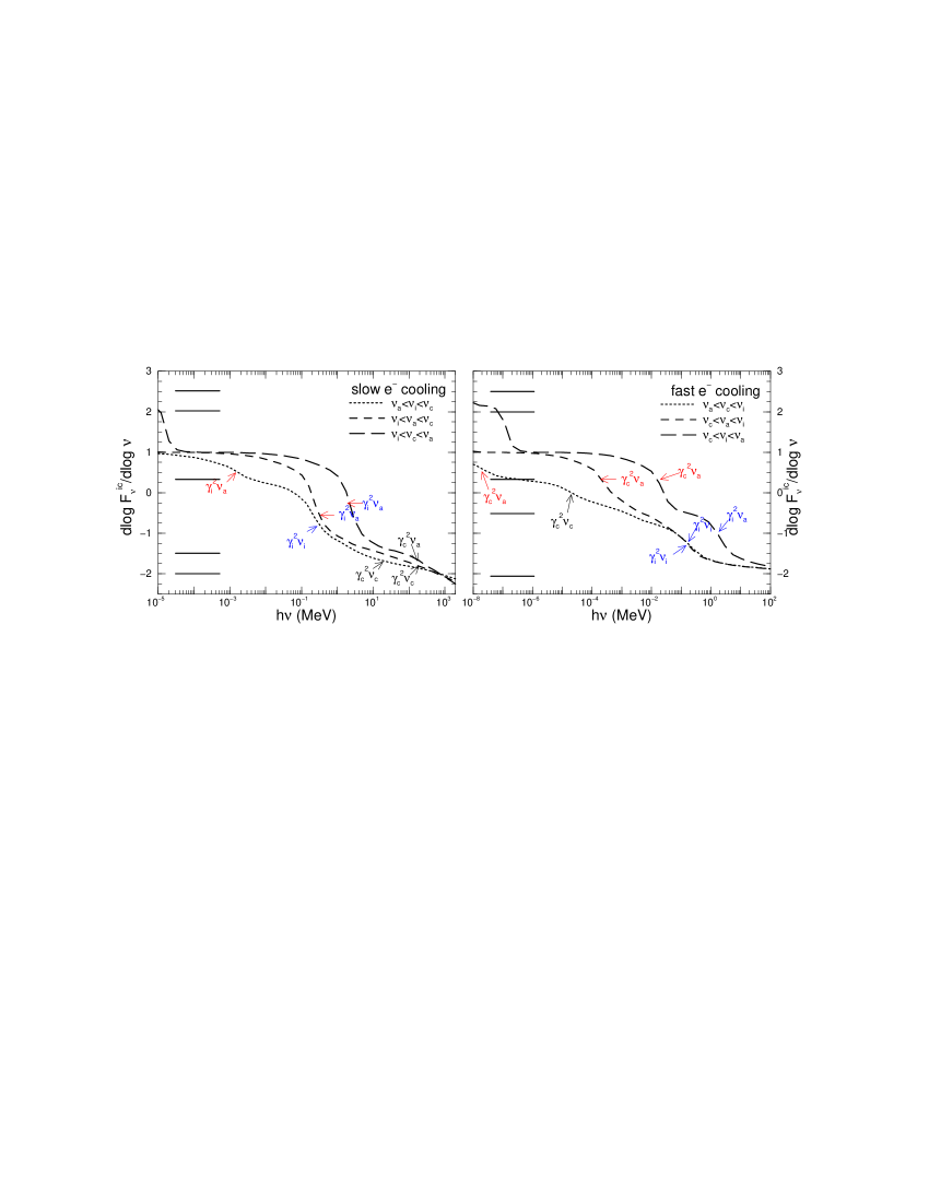
  Fig. 1.—: Slopes of IC spectra resulting from up-scattering of a broken power-law (four segments) synchrotron spectrum by a broken power-law distribution of electrons, for various possible combinations of synchrotron breaks: $\nu_{a}$ (absorption), $\nu_{i}$ (injection), and $\nu_{c}$ (cooling). Horizontal lines indicate the slopes of the synchrotron spectrum, which may be asymptotic values for the IC spectrum slope. Note that the IC emission below the lowest energy break indicated for each spectrum (red arrows), which results from up-scattering of self-absorbed synchrotron emission, is $F_{\nu}^{(ic)}\propto\nu$. Blue arrows/characters indicate the IC break frequency closest to the peak of the $\nu F_{\nu}^{(ic)}$ emission. Black arrows indicate less conspicuous breaks or IC frequencies that separate two asymptotic values of the IC spectral slope. A steep injected electron distribution with $p=4$ was used so that the IC breaks are easier to identify. IC spectra were calculated in the co-moving frame and blue-shifted by a factor 100.

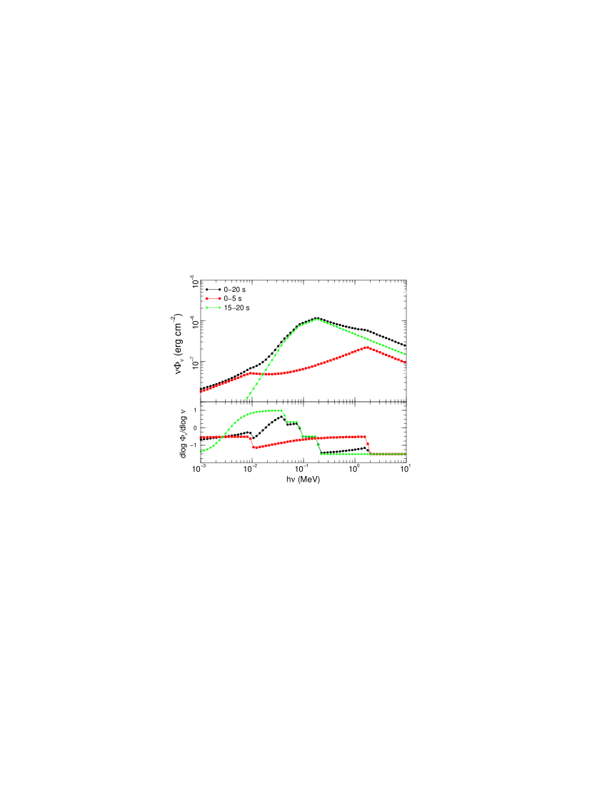
  Fig. 2.—: Time-integrated spectrum for a simulated burst produced by a wind consisting initially of 13 shells, whose ejection Lorentz factors has a log-normal distribution with $\Gamma_{0}=320$ and $A=1$ (see §2.1). Other wind parameters are: $t_{w}=10$ s, $L=3\times 10^{52}\;{\rm erg\,s^{-1}}$, $\varepsilon=0.15$, $\xi=10^{-5}$, $p=3$, redshift $z=1$ (see §2.2). The upper panel shows separately the spectra of the two structures exhibited by the light-curve, identified by the time ranges when they are seen, as well as the overall burst spectrum. Note the steepness of the $15-20\,{\rm s}$ spectrum below 40 keV peak (lower panel), due to up-scattering of self-absorbed synchrotron emission. The average dissipation efficiency per collision is $\theta=13\%$. Approximately 29% of the wind energy is eventually dissipated, out of which $\sim$ 4% is stored in electrons. About 50% of the electron energy is lost adiabatically, therefore the bolometric radiative efficiency of the burst is only 2.0%. The efficiency at which the wind converts its kinetic energy into 20 keV–1 MeV photons is 1.2%, due to that only 60% of the total emission falls in this energy range.

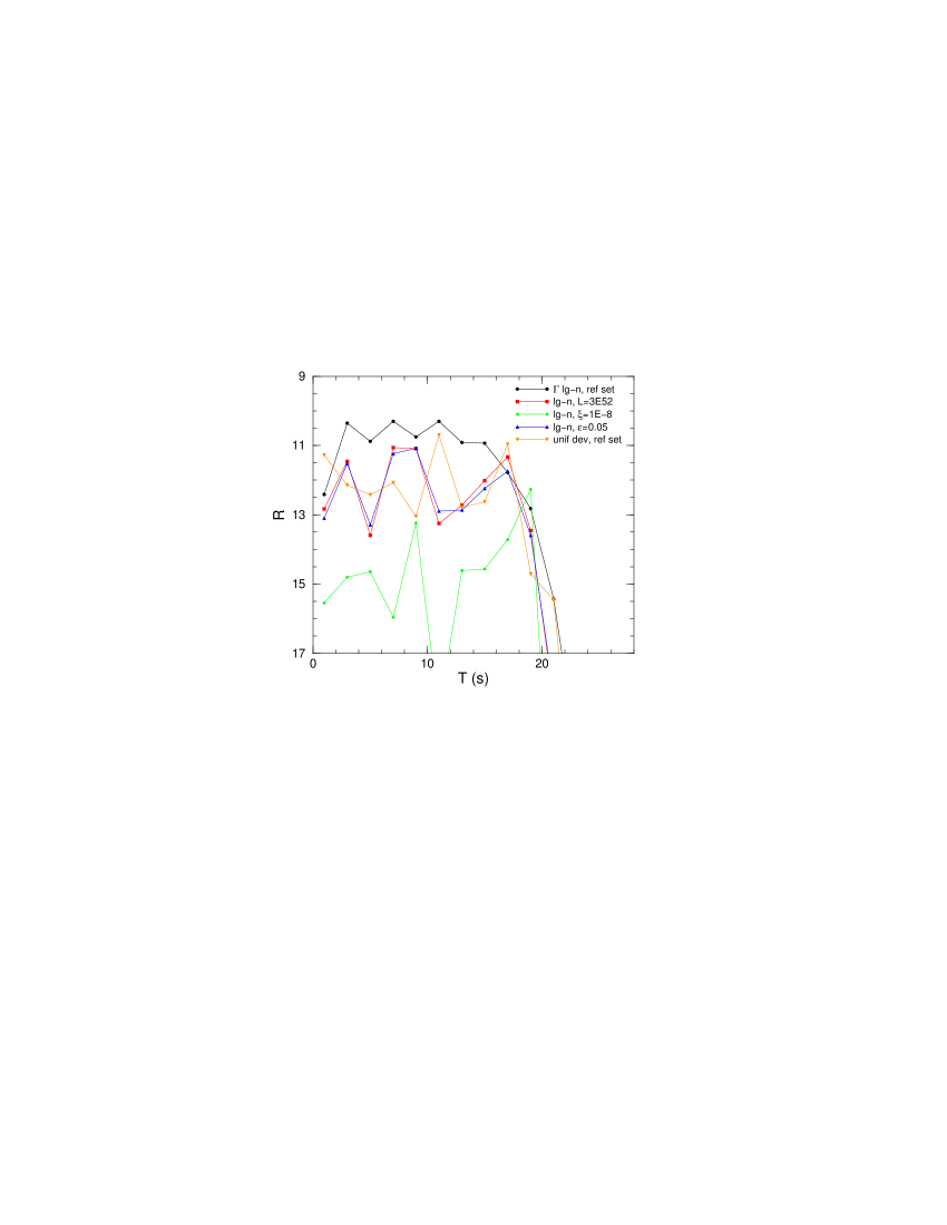
  Fig. 3.—: $R$-band magnitude of burst optical counterparts for few model parameters, bined in $2\,{\rm s}$ time intervals. The reference set is $t_{w}=10$ s, $L=10^{53}\;{\rm erg\,s^{-1}}$, $\varepsilon=0.15$, $\xi=10^{-5}$, $p=3$, redshift $z=1$ and 100 ejected shells. $\Gamma_{0}=320$ and $A=1$ for $\Gamma$ log-normal distributed, while for the uniform deviate $\Gamma$ is randomly distributed between 50 and $10^{3}$. The bursts last for about $(1+z)t_{w}=20$ s, exhibit 20–35 peaks, have spectral features (low and high energy spectral slope, break frequency) consistent to those found by Preece et al. 2000 in real bursts, 20 keV–1 MeV fluences in the range $(2-8)\times 10^{-6}\;{\rm erg\,cm^{-2}}$, and efficiencies of radiating the wind total energy in the BATSE range between 0.3% and 1%.