Is it Round? Spectropolarimetry of the Type II-P Supernova 1999em

Abstract

We present the first multi-epoch spectropolarimetry of a type II plateau supernova (SN II-P), with optical observations of SN 1999em on days 7, 40, 49, 159, and 163 after discovery. These data are used to probe the geometry of the electron-scattering atmosphere before, during, and after the plateau phase, which ended roughly 90 days after discovery. Weak continuum polarization with an unchanging polarization angle ($\theta\approx 160^{\circ}$) is detected at all epochs, with $p\approx 0.2\%$ on day 7, $p\approx 0.3\%$ on days 40 and 49, and $p\approx 0.5\%$ in the final observations. Distinct polarization modulations across strong line features are present on days 40, 49, 159, and 163. Uncorrected for interstellar polarization (which is believed to be quite small), polarization peaks are associated with strong P-Cygni absorption troughs and nearly complete depolarization is seen across the H$\alpha$ emission profile. The temporal evolution of the continuum polarization and sharp changes across lines indicate polarization intrinsic to SN 1999em. When modeled in terms of the oblate, electron-scattering atmospheres of Höflich, the observed polarization suggests an asphericity of at least $7\%$ during the period studied. The temporal polarization increase may indicate greater asphericity deeper into the ejecta. We discuss the implications of asphericity on the use of type II-P supernovae as primary extragalactic distance indicators through the Expanding Photosphere Method (EPM). If asphericity produces directionally dependant flux and peculiar galaxy motions are characterized by $\sigma_{v_{rec}}=300$ km s^-1, it is shown that the agreement between previous EPM measurements of SNe II and distances to the host galaxies predicted by a linear Hubble law restrict mean SN II asphericity to values less than $30\%$ ($3\sigma$) during the photospheric phase.

1 INTRODUCTION

The assumption of spherical symmetry in core-collapse supernova (SN) explosions is under assault. On the observational front, high-velocity “bullets” of matter in SN remnants (e.g., Taylor, Manchester, & Lyne 1993), the Galactic distribution (Lyne 1998) and high velocities of pulsars (Strom et al. 1995; Cordes & Chernoff 1998), the aspherical morphology of many young SN remnants (Manchester 1987; see, however, Gaensler 1998), and the asymmetric distribution of material inferred from direct speckle imaging of young supernovae (SNe; e.g., SN 1987A, Papaliolios et al. 1989; see, however, Höflich 1990) collectively argue for asymmetry in the explosion mechanism and/or distribution of SN ejecta. Moreover, recent advances in the understanding of the hydrodynamics and distribution of material in the preexplosion core (Bazan & Arnett 1994; Lai & Goldreich 2000) coupled with results obtained through multidimensional numerical explosion models (Burrows, Hayes, & Fryxell 1995) imply that asphericity may be a generic feature of the explosion process (Burrows 2000). It has even recently been proposed that some core-collapse SNe produce gamma-ray bursts (e.g., Bloom et al. 1999) through the action of a jet of material aimed fortuitously at the observer, the result of a “bipolar”, jet-induced, SN explosion (Khokhlov et al. 1999; MacFadyan & Woosley 1999; Wheeler et al. 2000). Such ideas shake the theoretical foundation of the conventional spherical neutrino-driven SN explosion (Colgate & White 1966), and beg for a direct observational probe of early-time SN geometry.

Shapiro & Sutherland (1982) first proposed that polarimetry could provide a powerful tool with which to study of young SN geometry. The most basic question is whether the SN is round. Because electron scattering dominates the opacity of SNe during the photospheric phase (Branch 1980), any continuum radiation that emerges at an angle to the surface normal is linearly polarized. For a spherical source that is unresolved (true for all young, recent SNe) the electric vectors cancel exactly, resulting in zero net polarization. Aspherical sources, however, will yield residual polarization due to incomplete cancellation; see Figure 1 of Leonard, Filippenko, & Matheson (2000b). In general, linear polarizations of $\sim 1\%$ are expected for moderate ($\sim 20\%$) SN asphericity. The exact polarization amount varies with the degree of asphericity, as well as with the viewing angle and the extension and density profile of the electron-scattering atmosphere (Höflich 1991a [H91]; Höflich 1995).

SNe come in many varieties, with the main classification based on the presence (type II) or absence (type I) of hydrogen in the spectrum near maximum light (see Filippenko 1997 for a recent review). Except for SNe Ia, whose progenitors are carbon-oxygen white dwarfs that accrete matter from a companion and undergo thermonuclear runaway, all other SN types (II-P, II-L, IIn, IIb, Ib, Ic) are believed to result from the explosion of evolved, massive stars (initial mass $\gtrsim 8-10\ M_{\odot}$) that have reached the ends of their nuclear-burning lives. These core-collapse events present a smorgasbord of spectral and photometric properties, leading to a proliferation of subclassifications. A consensus is emerging, however, that much of this diversity is due to the state of the progenitor’s hydrogen envelope (helium as well in some cases) and immediate circumstellar environment (CSE) at the time of the explosion.

“Normal” core-collapse events are thought to result from isolated stars with thick hydrogen envelopes (generally of several solar masses) intact at the time of the explosion. Their light curves show a distinct plateau (hence the moniker “SN II-P”), resulting from an enduring period (sometimes as long as 150 days) of nearly constant luminosity as the hydrogen recombination wave recedes through the envelope and slowly releases the trapped, shock-deposited energy. The spectral and photometric evolution of SNe II-P has been successfully reproduced by computer simulations of exploding red supergiant stars (e.g., Eastman, Schmidt, & Kirshner 1996; Weaver & Woosley 1993; Imshennik & Nadyozhin 1974; Eastman et al. 1994; Popov 1993). The basic model includes a source of thermal photons that electron-scatter their way out of the envelope (Branch 1980), with line features imprinted onto the continuum by resonance scattering in the envelope (see, e.g., Branch et al. 2000). The line features in photospheric-phase SNe are characterized by “P-Cygni” profiles, with blueshifted absorption troughs with emission centered near the rest wavelength. These characteristics are common for lines formed in expanding atmospheres. The general situation is illustrated by Figure 1. The absorption component results from continuum photons being scattered out of the line-of-sight (l-o-s) by gas approaching the observer in region 1. Photons scattered into the l-o-s by gas in regions 2 and 3 produce the emission component centered near the line’s rest wavelength, $\lambda_{\circ}$.

Figure 1: Schematic representation of an expanding SN atmosphere during the photospheric phase. Specific regions referred to in the text are indicated.

The observed properties of SNe II-P are consistent with those expected for a massive star exploding into the near-vacuum of the ambient interstellar medium. Some massive stars, however, cast off much of their hydrogen envelope prior to exploding, perhaps through stellar winds or due to the influence of a companion. It is the explosions of these stars that are believed to produce SNe II-L (“L” for their linearly declining light curves, lacking a plateau) or SNe IIn (“n” for the presence of relatively narrow emission lines lacking the customary P-Cygni absorption components [Schlegel 1990]). Much of the spectral peculiarity of these events likely results from the interaction between the SN and the dense CSE (Chugai 1997; Branch et al. 2000) in which the star explodes. Progenitors that have lost their entire hydrogen envelope well before the explosion produce SNe Ib (Type I due to the absence of hydrogen in their spectra), and those that have been stripped of both hydrogen and helium produce SNe Ic. Stars that explode with just a low-mass outer layer of hydrogen remaining are placed into the transitional category “SN IIb” since the spectrum shows hydrogen at early times but then becomes helium-dominated later on (e.g., SN 1993J; Matheson et al. 2000). It is possible, then, to roughly rank core-collapse events in order of increasing hydrogen envelope mass at the time of explosion: Ic, Ib, IIb, IIn, II-L and, finally, II-P. The exact sequence, especially the relative positions of IIb, IIn, and II-L, is still quite uncertain.

The geometry of SNe II-P are of particular interest due to their cosmological utility as extragalactic distance indicators through the Expanding Photosphere Method (EPM; Kirshner & Kwan 1974; Schmidt et al. 1994a [S94]), a variant of the Baade method used to measure distances to variable stars (Baade 1926). This technique is especially attractive since it is a primary distance indicator, unlike the “standard candle” method used to determine distances to SNe Ia. It is therefore not subject to all the uncertainties that plague the various rungs of the extragalactic distance ladder. Thus far, EPM has been applied to 18 SNe II spanning distances from 0.049 Mpc (SN 1987A) to 180 Mpc (SN 1992am; Schmidt et al. 1994b). Using SNe II alone, a Cepheid-independent value of $H_{0}=73\pm 7{\rm\ km\ s^{-1}\ Mpc^{-1}}$ has been derived (S94). However, unlike the empirically-based method used to measure distances to SNe Ia, distances derived to SNe II-P rely on the assumption of a spherically symmetric flux distribution during the early stages of development (i.e., the plateau). In this way, spectropolarimetry of SNe II-P provides a critical test of the cosmological utility of these core-collapse events.

Due largely to the difficulty of obtaining the required signal-to-noise (S/N) ratio, detailed spectropolarimetric studies exist for only three events, SN 1987A (Jeffery 1991a and references therein), SN 1993J (Trammell, Hines, & Wheeler 1993; Höflich et al. 1996; Tran et al. 1997), and SN 1998S (Leonard et al. 2000a; Wang et al. 2000), none of which were of the classic II-P variety. SN 1987A resulted from the explosion of a blue supergiant, and had a peak intrinsic polarization of $p\approx 0.7\%$ during the first 100 days. SN 1993J, a Type IIb event, was polarized at $p\approx 1.5\%$ at early times. SN 1998S, a peculiar Type IIn event, was polarized up to $3\%$ at early times. The polarization seen in these three objects suggests that core-collapse events, at least those of the unusual varieties represented by them, may indeed be aspherical at early times. It is also curious that SN 1993J and SN 1998S, which had both lost much of their hydrogen envelopes prior to exploding, were significantly more polarized than SN 1987A, which likely had retained most of its envelope. This trend is also seen in the sample of broadband polarimetric studies (or low S/N ratio spectropolarimetry) that have been carried out on SNe (Wang et al. 1996; see Wheeler [2000] for a comprehensive list of polarimetric observations of SNe), and tentatively suggests that the degree of polarization increases with decreasing envelope mass (Wheeler 2000). In fact, a polarization of nearly $7\%$ has recently been inferred for a SN Ic (Wang et al. 2000a).

It seems that the deeper we peer into the SN atmosphere, the more evidence there is for asphericity. This leads naturally to the conclusion that it is the collapse or explosion mechanism itself that is strongly asymmetric, and that evidence for this asymmetry is damped by the addition of outer envelope material (e.g., Chevalier & Soker 1989). Since a SN II-P gradually reveals its inner layers as the recombination front recedes through the hydrogen envelope during the plateau phase, a single object observed at multiple epochs during (and after) the plateau era provides an important test of this hypothesis: explosion asymmetry should result in increasing evidence for asphericity with time. With the larger aperture telescopes capable of generating high S/N ratio spectropolarimetry in reasonable observing times now available (e.g., Keck, VLT), the time is ripe for a detailed investigation into early-time SN II-P geometry.

Supernova (SN) 1999em was discovered on 1999 October 29 UT by Li (1999) at an unfiltered magnitude of $m\approx 13.5$ mag in the nearly face-on ($i\approx 31^{\circ}$, from LEDA) SBc galaxy NGC 1637 (Fig. 2). It was quickly identified as a Type II event, with prominent P-Cygni features of hydrogen Balmer and He I $\lambda$5876 and a blue continuum (Jha et al. 1999). Immediately after discovery a spectral, spectropolarimetric, and photometric campaign was initiated at Lick Observatory. Nearly daily optical photometry and spectroscopy of the young SN were obtained with the Katzman Automatic Imaging Telescope (KAIT) and the Lick 1-m Nickel reflector, respectively, providing unprecedented temporal coverage of this Type II event during the photospheric phase. Spectropolarimetry was obtained using the Lick 3-m and Keck-I 10-m telescopes.

We focus here on the spectropolarimetric observations of SN 1999em, and defer a more detailed discussion of the photometric and spectral data to a separate paper (Leonard et al. 2001), in which the EPM distance to SN 1999em ($d\approx 6$ Mpc) is derived. For our present purposes, we note that both its light-curve shape and spectral properties firmly establish SN 1999em as a Type II-P event, with a plateau lasting roughly 90 days from discovery. In addition, the EPM analysis determines the time of explosion to be $t_{\circ}\approx 5$ days before discovery, consistent with the absence of the SN in a CCD image of NGC 1637 taken 9 days before discovery (limiting magnitude about 19; Li 1999). We note that at an estimated distance of $\sim 6$ Mpc, SN 1999em reached an extinction-corrected ($E[B-V]=0.05$ mag [Baron et al. 2000]) peak $B$-band magnitude of $M_{B}=-15.3\pm 0.2$ mag, which is somewhat fainter than average for SNe II-P (Patat et al. 1994). Its color evolution may also have been somewhat unusual (Leonard et al. 2001). SNe II-P are known to be a heterogeneous class of objects, and these differences set a cautionary note on generalizing about the Type II-P class as a whole based on our findings for this one object.

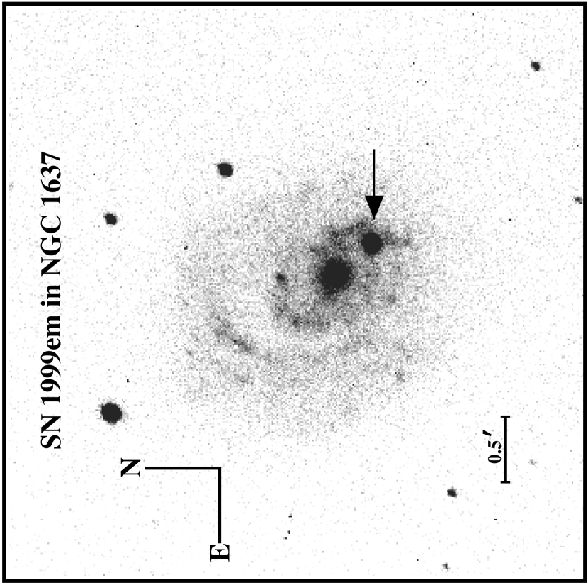
Figure 2: $B$-band image of NGC 1637 taken on 1999 October 31 with the Katzman Automatic Imaging Telescope (Treffers et al. 1997; A. V. Filippenko et al., in preparation). SN 1999em (arrow) is measured to be $15.\arcsec 1$ west and $17.\arcsec 2$ south of the galaxy nucleus (cf., Jha et al. 1999).

We obtained spectropolarimetry of SN 1999em on five occasions, with observations on days 7, 40, 49, 159, and 163 after discovery. We outline the observations and basic reduction techniques in § 2 and present the data in § 3. Section 4 discusses the spectropolarimetry, the total flux spectra, and the implications of asphericity on the use of SNe II-P as extragalactic distance indicators through EPM. Conclusions are summarized in § 5. Details of the data reduction process and a discussion of the interpretation of low-polarization spectropolarimetry similar to what is found for SN 1999em are given in Appendix A. Some preliminary results of this study were announced by Leonard, Filippenko, & Chornock (1999) and summarized by Leonard, Filippenko, & Matheson (2000b).

2 Observations and Reductions

We obtained spectropolarimetry of SN 1999em in 1999 on November 5, December 8, and December 17 (7, 40, and 49 days after discovery, respectively) with the Kast double spectrograph (Miller & Stone 1993) with polarimeter at the Cassegrain focus of the Shane 3-m telescope at Lick Observatory. Similarly, on 2000 April 5 and 9 (159 and 163 days after discovery, respectively), we used the Low-Resolution Imaging Spectrometer (Oke et al. 1995) in polarimetry mode (Cohen 1996) at the Cassegrain focus of the Keck-I 10-m telescope. The slit position angle (P.A.) was generally set near the parallactic angle (Filippenko 1982) for the midpoint of each set of observations in order to minimize differential light loss. A journal of observations is given in Table 1.

One-dimensional sky-subtracted spectra were extracted optimally (Horne 1986), with a width of from 3 to 5 times the full width at half maximum (FWHM) of the object’s spatial profile (i.e., the “seeing,” although guiding errors and dome turbulence can also contribute). This extraction width was found to represent a good compromise between the increased signal-to-noise (S/N) ratio obtained with wide extractions and the reduction of galaxy light contamination achieved using a narrow aperture. We subtracted a linear interpolation of the median values of background windows on either side of the object from the object’s spectrum; since the polarimetry optics restrict the useful (unvignetted) slit length to only $40^{\prime\prime}$ at Lick and $20^{\prime\prime}$ at Keck, background regions were necessarily quite narrow and close to the object. Each spectrum was then wavelength and flux calibrated, corrected for continuum atmospheric extinction and telluric absorption bands (Wade & Horne 1988), and rebinned to a 2 Å bin^-1 linear scale. Details of the extractions are given in Table 2.

We performed polarimetric analysis according to the methods outlined by Miller, Robinson, & Goodrich (1988) and Cohen et al. (1997). The P.A. offset between the half-wave plate and the sky coordinate system was determined for each observing run using polarized standard stars from the lists of Hiltner (1956), Mathewson & Ford (1970), Hsu & Breger (1982), and Schmidt, Elston, & Lupie (1992b). The absolute P.A. adopted for the standards is given in Table 3, along with the polarization angle measured for other polarized standards observed, but not used to determine the offset. When multiple polarization standards were observed on the same night, they always agreed to within $\pm 0.5^{\circ}$.

There were a few peculiarities encountered in the reductions. Briefly, on day 7, we used a dichroic filter that split the spectrum at about 5500 Å and sent the light to separate gratings that dispersed the spectra in the blue and red arms of the spectrograph. This yielded spectral coverage from 3400 Å to 7700 Å, but the region around the dichroic cutoff ($5100-6000$ Å) suffered from irregularities at the $1\%$ level that did not calibrate out of the polarimetry; thus, we discarded the range $5100-6000$ Å in the polarimetric analysis. In addition, instrumental polarization ranging up to $\sim 0.4\%$ was detected at blue wavelengths ($\lambda\lesssim 5000$ Å) in this setup and had to be removed using the observation of the null standard on this night. On days 40 and 49 we observed without the dichroic and obtained continuous coverage over $4300-7000$ Å using only the red arm of the spectrograph. Observations of the null standards HR 7783 and HR 8086 on day 49 showed a flat, well-behaved polarization response. A small polarization ($<0.2\%$) was measured to both nulls. However, observations of these “nulls” on nights when additional null standards were observed suggest that much of this polarization is likely intrinsic to the stars themselves (i.e., the interstellar medium along the line-of-sight [l-o-s]) and not of instrumental origin. Therefore, we did not apply any instrumental correction to the data from these nights. Observations of null standards at Keck were always found to be null to within 0.1%, suggesting negligible instrumental polarization in the day 159 and 163 data. On day 159, a CCD readout failure occurred during the observation of the final waveplate position ($67.5^{\circ}$), leaving us with only 3 of the desired 4 observations in the set. While it was still possible to derive the Stokes parameters, the data had potential systematic errors. Fortunately, SN 1999em was observed again just four days later at Keck, largely confirming the results of the earlier observation. A complete discussion of these issues, along with an investigation into sources of systematic uncertainty in measurements of SN polarization, is given in Appendix A.

The displayed polarization $p$ is the “rotated Stokes parameter” (RSP), calculated by rotating the normalized Stokes parameters $q$ and $u$ by a fit to the continuum P.A. curve so that all of the continuum polarization falls in a single Stokes parameter (here, rotated $q$). This is preferable to calculating either the “traditional” $p$ ($p_{trad}\equiv\sqrt{q^{2}+u^{2}}$), or a “debiased” $p$ ($p_{deb}\equiv\pm\sqrt{\mid q^{2}+u^{2}-(\sigma^{2}_{q}+\sigma^{2}_{u})\mid}$, where $p_{deb}$ assumes the sign of [$q^{2}+u^{2}-\sigma^{2}_{q}-\sigma^{2}_{u}$]; see Stockman & Angel 1978), since the former is biased high and is positive-definite while the latter gives poor results for data with low $p/\sigma_{p}$ (e.g., Miller et al. 1988). RSP provides a good measure of $p$ when the P.A. is a slowly varying function of wavelength. However, when there are sharp P.A. rotations across line features, RSP always underestimates the true polarization, and it is necessary to examine both RSP and URSP (rotated $u$) to determine the line’s polarization. To measure absorption-line and emission-line polarizations, we first binned the flux data into 10 Å (rest) bins (about 1.5 resolution elements wide for the standard Lick and Keck setups), and then derived $q$ and $u$ from the binned data. Although binning always reduces peak polarization, it is more reliable because of the reduced noise, which is especially problematic here since polarization peaks are often associated with line troughs. However, since features may be quite sharp, it often happens that the polarization change is detectable in only a few (rebinned) pixels. In such cases, we carefully examine the polarization properties of the original spectrum (always binned 2 Å bin^-1) to see if the polarization feature is seen consistently across many pixels or is due to a single deviant pixel, before concluding that a true polarization change exists. We determined observed $B$-band and $V$-band polarization by calculating the “debiased”, flux-weighted averages of $q$ and $u$ over the intervals $3950-4900$ Å and $5050-5950$ Å, respectively, converting to $p$ and $\theta$ only at the final step for quoting results. A more extensive description of the adopted analysis techniques is given in Appendix A.

3 Results

Figures 3, 4, 5, and 6 show the observed polarization data for SN 1999em on days 7, 40, 49, and 161 (a combination of the observations on day 159 and 163) after discovery. The data from days 7, 40, and 49 are the weighted averages of two successive observations taken on those nights, and the “day 161” data are the weighted average of data obtained on days 159 and 163; see Appendix A for details. A montage of all the epochs studied is shown in Figure 7. Measured values for the observed $V$-band polarization are given in Table 4, along with line trough polarization for Fe II $\lambda 5169$ and Na I D $\lambda\lambda 5890,5896$, and the approximate polarization change measured across the H$\alpha$ profile.

The day 7 flux spectrum shows features that are typical for a very young SN II-P: a blue continuum with P-Cygni lines of hydrogen Balmer and He I $\lambda 5876$. The blue edges of absorption troughs indicate velocities in excess of $10,000{\rm\ km\ s}^{-1}$ for the fastest moving gas. The spectra from days 40 and 49 are typical for a SN II-P during the plateau phase, characterized by a thermal continuum with P-Cygni hydrogen Balmer, Fe II $\lambda\lambda 4924,5018,5169$, Sc II $\lambda\lambda 5526,5657,6245$, and Na I D $\lambda\lambda 5890,5896$. The plateau phase for SN 1999em lasted until about 90 days after discovery, suggesting that a massive hydrogen envelope remained at the time of explosion (Leonard et al. 2001). The day 161 spectrum is emission-line dominated, with prominent H$\alpha$ and [Ca II] $\lambda\lambda 7291,7324$, implying that the transition to the nebular phase was underway; P-Cygni absorptions still indicate significant continuum light, however, and the fully nebular phase is not expected until after about day 300 (e.g., Jeffery 1991a).

Figure 3: Polarization data for SN 1999em, obtained 1999 November 5, only 7 days after discovery. In this, and all subsequent figures, the NED recession velocity of 717 km s^-1 has been removed. Instrumental polarization at blue wavelengths has been removed from the data on this night only (see Appendix A). (a) Total flux, in units of $10^{-15}$ ergs s^-1 cm^-2 Å^-1. (b) Observed degree of polarization. (c) Polarization angle in the plane of the sky. (d, e) The normalized $q$ and $u$ Stokes parameters. (f) Average of the (nearly identical) $1\sigma$ statistical uncertainties in the Stokes $q$ and $u$ parameters for the displayed binning of 2 Å bin^-1. The polarization shown in this and all plots is actually the “rotated Stokes parameter” (RSP; see Appendix B). To facilitate comparison, the ordinate ranges of panels (b), (c), (d), (e), and (f) are the same in Figures 3, 4, and  5.

Figure 4: As in Figure 3, but for data obtained on 1999 December 8.

Figure 5: As in Figure 3, but for data obtained on 1999 December 17.

Figure 6: As in Figure 3, but for the weighted average of polarization data obtained on 2000 April 5 and 9, 159 and 163 days after discovery, respectively.

Figure 7: Montage of the observed optical polarization of SN 1999em, with arbitrarily scaled total flux spectra (thick lines) overplotted for comparison of features. The polarization spectra are binned 5 Å bin^-1 to improve the S/N ratio.

4 Analysis and Discussion

4.1 Spectropolarimetry

4.1.1 Introduction

We interpret the spectropolarimetry of SN 1999em in terms of the physical picture shown (for a spherical atmosphere) in Figure 1, and described in § 1. Early theoretical work on SN spectropolarimetry was stimulated by observations of SN 1987A. Investigators initially proposed that the observed polarization (up to $p_{V}\approx 0.7\%$ during the first 100 days after explosion) was due to the polarizing effect of line scattering (Jeffery 1989). It was soon realized, however, that scattering by free electrons extending out into the line-forming regions of the envelope dominates the overall polarization level of photospheric SNe (H91), and that weak collisions in the line-forming region of the SN atmosphere tend to destroy the intrinsic line polarizing effect, except perhaps in the outer regions of the atmosphere at late times (Jeffery 1991b). The loss of geometric information caused by the collisions generally produces unpolarized emission components for the P-Cygni line profiles, an assumption often used to constrain the interstellar polarization (ISP; see, e.g., Leonard et al. 2000a). Detailed models specific to SN 1987A suggest that the net polarization seen was likely produced by a modest asphericity of about $10\%-20\%$ (Jeffery 1991b; H91; see also Wang & Wheeler 1996).

Translating observed SN continuum polarization into an estimate of the asphericity of the electron-scattering atmosphere is quite model-dependent. The original problem of the polarization of light emerging from a semi-infinite, plane-parallel, pure electron scattering atmosphere with constant net flux was solved by Chandrasekhar (1946). The first attempt to apply the formalism to SNe was by Shapiro & Sutherland (1982), who solved it for a plane-parallel, optically-thick, electron-scattering atmosphere wrapped around an ellipsoid. The plane-parallel model, however, requires extreme asymmetry to produce even modest polarization: to get $p=1\%$ demands an asphericity of at least 60% (the percent asphericity is defined here as $(1-[a/b])\times 100$, where $a$ and $b$ are the semiminor and semimajor axis lengths, respectively) for the oblate case; prolate spheroids are unable to produce polarization of more than 0.77% for any axis ratio or viewing angle. Realistic models of the extended atmospheres of SNe, however, have recently been shown to be more polarizing than the plane-parallel approximation predicts.

There are many factors that can influence the degree of SN continuum polarization. The most recent, general study of the polarization expected from an aspherical SN atmosphere is H91, in which the continuum polarization resulting from an axially symmetric (either oblate or prolate), electron-scattering dominated photosphere is calculated as a function of the photosphere’s geometry and size relative to the envelope, the scattering atmosphere’s optical depth and density profile, and the axial ratio of the envelope. Particularly useful is the lower bound placed on the asphericity implied by polarization measurements: by fixing all other parameters to maximize the resulting polarization (i.e., scattering optical depth = 1, continuum region physically small compared with envelope, object viewed equator-on), the maximum polarization as a function of axis ratio is produced (Figure 4 of H91). Determination of intrinsic SN continuum polarization can thus lead to a lower limit on the implied asphericity of the scattering atmosphere from this model.

In addition to the information gleaned from the continuum polarization level, sharp polarization changes across strong line features can also contain a wealth of information about the geometry of the scattering environment. The influence of asphericity on the polarization properties of P-Cygni lines was first addressed in detail by McCall (1984), who predicted that polarization should increase in the absorption troughs. His basic idea is that P-Cygni absorption by gas in region 1 (Fig. 1) selectively blocks photons coming from the central, more forward-scattered (hence less polarized) regions, thereby enhancing the relative contribution of the more highly polarized photons from the limb (i.e., from regions 2 and 3 in Fig. 1; see also Fig. 1 of Leonard et al. 2000b). Jeffery (1991b) extended the argument by predicting drops in polarization at the location of emission peaks due to the dilution of the polarized continuum light by unpolarized emission-line photons.

The basic prediction, then, is that a “reverse” P-Cygni polarization profile should characterize strong P-Cygni line features formed above or within an aspherical electron-scattering atmosphere. (We note that polarization increases in P-Cygni absorption troughs are often seen in spectropolarimetric studies of broad absorption line QSOs, and are generally given a similar physical interpretation [e.g., Brotherton et al. 1997; Ogle et al. 1999]). Taking the limiting case of blockage of only unpolarized light (or light with electric vectors that exactly cancel) in a line trough and addition of completely unpolarized light in a line peak, the polarization change expected across a P-Cygni feature from this admittedly simple model is

$$p_{trough}\leq p_{max}=p_{cont}\times\frac{I_{cont}}{I_{trough}},$$ (1)

$$p_{peak}\geq p_{min}=p_{cont}\times\frac{I_{cont}}{I_{peak}},$$ (2)

where $p_{cont}$ is the continuum polarization and $I_{cont},I_{peak},{\rm\ and\ }I_{trough}$ represent the flux intensity in the continuum, line peak, and line trough, respectively. The continuum polarization and the continuum flux intensity are both interpolated from the continuum regions surrounding the line.

In general, the polarization observed across a P-Cygni profile will differ from that predicted by equations (1) and (2). The most important factor neglected by the simple geometric argument is the influence that resonance scattering of continuum photons has on the polarization properties of the line profile. In a SN atmosphere, continuum photons that are resonantly scattered by a line are unpolarized (Jeffery 1991b; Höflich et al. 1996), and will diminish the polarization level throughout the entire P-Cygni profile. This depolarizing effect will be especially pronounced in lines that are optically thick throughout the envelope, such as H$\alpha$. In addition, the strong emission component of H$\alpha$ will tend to fill in the absorption trough, increasing $I_{trough}$. Countering this is the polarization that line photons themselves may acquire upon being scattered by free electrons, which likely exist in the line-formation region itself (Höflich et al. 1996 ). A final reason that the polarization measured will differ from that predicted is purely observational: since the P-Cygni absorption features in SNe II-P are quite sharp (the FWHM of the absorptions in SN 1999em due to prominent metal lines on day 49, for example, are all in the range $35-45$ Å), the typical grating-CCD resolution of $5-10$ Å coupled with the coarse binning needed to improve the statistics inevitably reduces measured peak polarization values. Indeed, in the limit of infinite bin size, $p_{trough}\rightarrow p_{cont}$.

There are thus several mechanisms in addition to the simple geometric model that may contribute to the polarization measured across a P-Cygni line feature and it is not obvious which should dominate. In this regard, it is instructive to study the characteristics of the line polarization presented by the detailed spectropolarimetric studies of SN 1987A (Jeffery 1991a, 1991b), SN 1993J (Trammell et al. 1993; Höflich et al. 1996 ; Tran et al. 1997), and SN 1998S (Leonard et al. 2000a).

For SN 1987A, many epochs of the ISP-subtracted data show large polarization increases at the locations of P-Cygni absorptions due to H$\gamma$, H$\beta$, Fe II $\lambda 5169$, Na I D $\lambda\lambda 5890,5896$, Ca II $\lambda\lambda 8498,8542,8662$, and possibly Fe II $\lambda 5018$ and H$\alpha$ as well (see Jeffery 1991a and references therein). Polarization decreases occur across the emission peaks of H$\alpha$ and Ca II $\lambda\lambda 8498,8542,8662$. Since error bars are not given and the polarization data were evidently not corrected for statistical biases, it is somewhat difficult to quantitatively assess the polarization changes (especially the trough increases) seen across the lines. Taken at face value, though, none of the trough increases appears to exceed the limit given by equation (1). Polarization decreases across H$\alpha$, however, do occasionally go below the limit set by equation (2).

The three ISP-subtracted spectropolarimetric epochs of SN 1993J (Type IIb) presented by Tran et al. (1997) also show distinct polarization increases in the absorption troughs of H$\beta$, Fe II $\lambda 5169$, and He I $\lambda 5876$ (probably blended with Na I D $\lambda\lambda 5890,5896$), and polarization decreases across the He I $\lambda 5876$ and blended H$\alpha$/He I $\lambda 6678$ emission lines (the reverse P-Cygni profile across the He I $\lambda 5876$ is particularly pronounced). Detailed modeling of a single early-time spectropolarimetric epoch of SN 1993J presented by Höflich et al. 1996 successfully reproduces the depolarization across the entire H$\alpha$ profile, but does somewhat less well at fitting the He I/Na I D feature: whereas the model predicts a polarization decrease at the line’s absorption trough, the data indicate a small polarization rise. It is possible that the increased importance selective blocking of forward-scattered light has in lines of low optical depth contributes to the different polarization behavior seen here between H$\alpha$ and He I/Na I D.

Perhaps the clearest demonstration of the influence that unpolarized emission lines have on SN spectropolarimetry, however, is the single spectropolarimetric epoch of SN 1998S discussed by Leonard et al. (2000a). At the very early epoch studied (just 5 days after discovery), this peculiar Type IIn event displayed a smooth, blue continuum with superposed broad, symmetric emission lines lacking any absorption components. The spectropolarimetry was characterized by a flat, highly polarized ($p\approx 3\%$ after ISP removal) continuum with pronounced polarization decreases across all the emission features.

Aspects of the predicted reverse P-Cygni polarization profile are thus found in the spectropolarimetry of all previously studied SNe II. However, SN 1987A, SN 1993J, and SN 1998S were all quite unusual core-collapse events. SN 1993J and SN 1998S both showed strong spectroscopic evidence for interaction with circumstellar material. In addition to being a blue supergiant, the progenitor of SN 1987A may also have been spun up by a merger with a companion star prior to explosion (Collins et al. 1999). Such circumstances add complexity to the interpretation of spectropolarimetry. Since SN 1999em appears to be a relatively normal SN II-P, it presents a great opportunity to study the impact of asphericity on line polarization without any added complication by “external” influences.

4.1.2 Interstellar Polarization

A major source of uncertainty in SN spectropolarimetry is the degree to which interstellar dust along the l-o-s polarizes the SN light. An assumption often invoked to determine the ISP to SNe is that broad, resonance-scattered and recombination line photons (e.g., H$\alpha$) at early phases are intrinsically unpolarized; see § 4.1.1 for the theoretical underpinnings behind this assumption, and Appendix B for details of the application of this technique (see also Jeffery 1991b; Trammell et al. 1993; Höflich et al. 1996 ; Wang et al. 1996; Tran et al. 1997). With this assumption, the observed polarization of the emission-line photons is then entirely due to the ISP. Our earliest epoch, day 7, has very low continuum polarization and no obvious line features (see Fig. 12 for detail of the H$\alpha$ region). For H$\alpha$ emission from $6404$ to $6622$ Å ($\pm\ 5000{\rm\ km\ s}^{-1}$ from the deredshifted line peak at 6512 Å) and background regions $6000-6250$ Å and $6900-7500$ Å, we find $p({H\alpha})=0.08\pm 0.06\%{\rm\ at\ }\theta=171^{\circ}\pm 15^{\circ}$. This value is consistent with the continuum measured in the range $6900-7500$ Å ($p=0.12\pm 0.02\%{\rm\ at\ }\theta=153\pm 5^{\circ}$), and therefore allows for the possibility that all of the polarization seen is interstellar in origin. On the other hand, the polarization found is also marginally consistent with zero polarization, which would allow all of the observed polarization to be intrinsic to the SN. Our data therefore do not distinguish well between an ISP of 0.12% and an ISP of zero with this test. In any event, though, if H$\alpha$ emission-line photons are really intrinsically unpolarized at this early epoch, it does suggest very low ISP from dust in either the host galaxy or Milky Way (MW), with a formal $3\sigma$ upper limit of ${\rm ISP}<0.26\%$.

There are additional indications of low ISP contamination along the l-o-s to SN 1999em. First, since the same dust that polarizes also reddens SN light, with the maximum polarization always found to be less than $9E(B-V)$ for the MW (Serkowski, Mathewson, & Ford 1975), a small ISP for SN 1999em is consistent with its low Galactic reddening of $E(B-V)_{MW}=0.04$ mag (Schlegel, Finkbeiner, & Davis 1998), as well as with the total reddening of $E(B-V)_{tot}\approx 0.05$ mag estimated by Baron et al. (2000; see also Leonard et al. 2001) from theoretical fits to the early-time continuum shape. This reddening restricts the ISP to values less than $0.45\%$; we note, however, that the upper limit of $E({B}{\rm-}{V})=0.15$ mag given by Baron et al. (2000) is consistent with an ISP of up to $1.35\%$. Second, of the 11 stars with measured polarizations within $5^{\circ}$ of SN 1999em (Heiles 2000), six have zero polarization within their quoted uncertainties, and all have $p_{V}<0.2\%$, although only two (HD 29248 and HD 30112) lie sufficiently far away ($d>300{\rm\ pc\ }$) to fully sample the ISP through the Galactic plane. Third, even though $p$ increases through the 4 epochs, the polarization angle of SN 1999em remains nearly constant at $\theta\approx 160^{\circ}$. If the day 7 polarization was completely due to ISP it would suggest that $\theta_{ISP}=\theta_{SN}$, an unlikely chance occurrence. Furthermore, optical imaging polarimetry of face-on spirals (Scarrott, Rolph, & Semple 1990; Scarrott et al. 1991) generally shows polarization vectors aligned parallel to the spiral arms (i.e., perpendicular to the line connecting a point with the galaxy’s center), which would predict $\theta_{ISP}\approx 130^{\circ}$ given the location of SN 1999em in NGC 1637, somewhat far from the observed $\theta\approx 171^{\circ}$. Finally, the nearly complete depolarization across the H$\alpha$ line to $q\approx 0\%,u\approx 0\%$ on days 40, 49, and 161 (see Figs. 13, 14, 15) is consistent with a near-zero ISP from physical considerations discussed in the next section.

Therefore, while none of the preceding arguments is individually conclusive, taken together they suggest that polarimetry of SN 1999em is contaminated by a relatively small degree of ISP. Although impossible to know for sure, we suspect that the ISP is less than $0.3\%$, and cautiously proceed to analyze our data with no correction for its effects. We note that since ISP is a smoothly varying function of wavelength and is constant with time, uncertainty in its value affects neither temporal polarization changes nor modulations across specific line features. We caution, however, that any interpretation of polarization increases, decreases, or directional changes in line features is affected by the choice of ISP (see, e.g., Fig. 10 of Leonard et al. 2000a). Other sources of systematic uncertainty may add an additional $0.1\%$ uncertainty to the accuracy of the measured polarizations (see Appendix A).

4.1.3 SN 1999em

The broadband polarization of SN 1999em (generally, observed $V$) rises from $p~{}=~{}0.18\pm 0.01\%$ on day 7 to $p=0.53\pm 0.03\%$ on day 161 (Table 4 and Fig. 8a; quoted uncertainties are $1\sigma$ statistical only, and do not reflect systematic effects), suggesting a modest amount of intrinsic SN continuum polarization. The lack of any obvious wavelength dependence of the continuum polarization (e.g., Fig. 7) is consistent with an electron-scattering origin. A remarkable feature is that although the polarization level changes, it maintains a nearly constant polarization angle in the plane of the sky (Fig. 8b), similar to what was seen in SN 1987A (Jeffery 1991a). This strongly suggests that a preferred symmetry axis persists as the photosphere recedes and exposes ever deeper regions of the envelope. The change in polarization by $\sim 0.3\%$ from day 7 to day 161 cannot be produced by ISP, and is likely intrinsic to the SN itself. We note that the overall polarization level and characteristics of the line features are consistent with those reported by Wang et al. (2000b) for spectropolarimetry of SN 1999em obtained on day 72. The continuum polarization level implies a minimum asphericity of $\sim 7\%$ during the plateau era and $\sim 10\%$ on day 161 from the oblate, electron-scattering models of H91.

Figure 8: (a) Observed broadband polarization and (b) polarization position angle in the plane of the sky of SN 1999em as a function of time. Error bars are $1\sigma$ statistical for the observed $V$ band ($5050-5950$ Å) except for day 7, which is for observed $6050-6950$ Å. Note that although the polarization more than doubles during the first 161 days, the polarization angle remains fixed.

The temporal polarization increase may indicate increasing asphericity deeper into the SN ejecta. However, it is not clear that the models investigated by H91 are directly applicable for either very early or very late SN epochs. At early times (i.e., prior to the appearance of line features due to heavy metals; for SN 1999em this occurred on about day 9 (Leonard et al. 2001), the electron density profile above a SN II photosphere is believed to be very steep (see, e.g., Jeffery 1991b; Eastman et al. 1996; Matzner & McKee 1999). This type of atmosphere has much less polarizing power than one with the shallower electron density gradients typical of SN atmospheres during the recombination phase studied by H91. In fact, Jeffery (1991b) suggests that the shift from a steep to a shallow electron density gradient may explain the polarization rise seen in SN 1987A early on (from $p_{V}\approx 0.2\%{\rm\ to\ }p_{V}\approx 0.7\%$ over the first 30 days) without the need for any increase in asphericity. Höflich et al. 1996 cautiously propose the same mechanism to explain the early-time polarimetric behavior of SN 1993J as well. It is possible that a similar effect is at work in SN 1999em. The characteristics of the electron-scattering atmosphere during the transition to the nebular phase (i.e., day 161) also differ significantly from those modeled by H91. As SN 1999em ages the optical depth to electron scattering decreases; at some point in the nebular phase, in fact, it will drop well below 1, rendering spectropolarimetry ineffective as a geometric probe. It is possible that a reduced electron-scattering optical depth is responsible for the relatively low polarization measured at this late epoch.

While interpretation of the overall polarization level is hampered somewhat by possible ISP contamination and other sources of systematic uncertainty (Appendix A), the distinct polarization modulations across strong P-Cygni features are not. As anticipated (§ 4.1.1), sharp polarization peaks are associated in the later epochs with deep P-Cygni line troughs, most conspicuously Fe II $\lambda 5169$ and Na I D $\lambda\lambda 5890,5896$ (probably blended with Ba II $\lambda 5853$ and He I $\lambda 5876$ on day 161). We measure trough polarization in 10 Å bins to help improve the statistics in these low S/N ratio regions, and display the results in Figures 9, 10, 11 and in Table 4. The most dramatic increase is seen in the blended Na I D line on day 161, in which the measured RSP is $p=3.4\%\pm 1.4\%$, and the true polarization is likely even higher given the evidence for P.A. rotation found in its URSP (see Appendix B). The measured polarization increases in all troughs are in accord with the limit set by equation (1).

Figure 9: Detail of the region around the absorption trough of Fe II $\lambda 5169$ on 1999 December 17. (a) Normalized flux, displayed at 2 Å bin^-1. (b) Observed degree of polarization, measured as the rotated $q$ parameter. (c) Observed degree of polarization in the rotated $u$ parameter. Error bars in ($b$) and ($c$) are $1\sigma$ statistical for 10 Å bin^-1. In the absence of rapid P.A. change with wavelength, the URSP should scatter about zero; see Appendix B for details.

Figure 10: As in Figure 9, but for the weighted average of data obtained on 2000 April 5 and 9. The sharp spike in URSP at the bottom of the line trough may indicate that RSP underestimates the true trough polarization.

Figure 11: As in Figure 9, but for the weighted average of data obtained on 2000 April 5 and 9 near the absorption trough of Na I D $\lambda\lambda 5890,5896$ (Ba II $\lambda 5853$ and He I $\lambda 5876$ probably also contribute). Note that ${\rm URSP}\approx-1.7\%$ in many consecutive pixels near the absorption minimum, indicating that RSP may underestimate $p$ by as much as $0.4\%$.

The strong depolarization across the H$\alpha$ profile also implies intrinsic SN polarization (Figs. 12 through 15), with the change in polarization across the line increasing by $\sim 0.6\%$ during the first 161 days (Table 4). On days 40, 49, and 161, nearly complete depolarization exists from slightly redward of the flux absorption minimum to the line peak near $v\approx 0{\rm\ km\ s^{-1}}$. The fact that the depolarization goes well below the value expected from the simple model of dilution of polarized continuum light with unpolarized H$\alpha$ photons (eq. [2]) and the lack of a polarization increase associated with the H$\alpha$ trough may be due to a depressed underlying continuum polarization resulting from resonance scattering of continuum photons by H$\alpha$ (§ 4.1.1). In effect, since H$\alpha$ is optically thick throughout the atmosphere, it presents an absorbing screen that “covers” both the limb and the central regions (Fig. 1), unlike the optically thin metal lines (i.e., Fe II or Na I D) that predominantly block unpolarized (i.e., forward-scattered) light (§ 4.1.1). A similar H$\alpha$ depolarization was observed and theoretically modeled in SN 1993J (Höflich et al. 1996 ), and was seen in SN 1987A as well (Jeffery 1991a; see also § 4.1.1).

Figure 12: Region around H$\alpha$ on 1999 November 5. Error bars are $1\sigma$ statistical for 10 Å bin^-1. (a) Total flux, normalized by a spline fit to the continuum, displayed at 2 Å bin^-1 for better resolution. (b) Observed degree of polarization, determined by the rotated Stokes parameter (rotated $q$). (c) Observed degree of polarization in the rotated $u$ parameter. (d, e) Normalized $q$ and $u$ Stokes parameters. To facilitate comparison, the same ordinate ranges are used in Figures 12, 13, and 14.

Figure 13: As in Figure 12, but for data obtained on 1999 December 8. Note the depolarization evident across the emission profile.

Figure 14: As in Figure 12, but for data obtained on 1999 December 17. The depolarization seen across H$\alpha$ on day 40 (Figure 13) is evident here as well.

Figure 15: As in Figure 12, but for the weighted average of data obtained on 2000 April 5 and 9, and shown with an extended velocity range. The normalized polarized flux (RSP $\times f_{\lambda}$) is overplotted (thin line) in (a). Note the increased polarization in the red wing of the line.

On day 161 the polarization increases steadily through the red wing of the H$\alpha$ profile, reaching $p\approx 1.5\%$ at $v=5,000{\rm\ km\ s^{-1}}$, and then drops back to the continuum value at $v\gtrsim 12,000{\rm\ km\ s^{-1}}$. The polarized flux (shown overplotted in Fig. 15a) also peaks about 3200 km s^-1 to the red of the nominal line center. One agent that may contribute is the redshift that line photons acquire upon being scattered by electrons moving away from the point of origin (i.e., the expanding universe paradigm; see, e.g., Bailey 1988; Witteborn et al. 1989). Another possibility is that at this late epoch the density and temperature conditions in the outer atmosphere are such that the depolarizing effect of weak collisions is reduced, allowing the intrinsic line polarizing effect due to resonance scattering to contribute (see Jeffery 1989, 1990 for a thorough analysis of polarized line radiative transfer in an expanding atmosphere). A final, intriguing possibility is that H$\alpha$ photons on the “far” side of the expanding SN (region 4 in Fig. 1), are scattered into the l-o-s by electrons in region 3. Although at this late epoch the physical size of region 4 is quite small and would contribute little flux, the photons would be highly polarized due to the near $90^{\circ}$ scatter they suffer, perhaps allowing them to significantly affect the polarization of the line’s red wing.

The existence of a broad, strong, polarized emission line allows us to investigate a key question about the line-scattering region’s geometry: is it axisymmetric? That is, does the line profile present a uniform polarization angle in the plane of the sky? The best way to test this is to follow the path traced by the data in the $q$-$u$ plane, since a common axis of symmetry for the different scattering regions will result in a linear path. This method is preferred over simply looking to see if the polarization angle changes across the line (i.e., $\theta$ in Fig. 6), since ISP can produce apparent P.A. rotations, but will not alter the shape of the path in $q$-$u$. Figure 16 shows the results for H$\alpha$ on day 161, extending from $0$ to $5000{\rm\ km\ s^{-1}}$. The path traced by the red side of the profile is quite linear, and the polarization angle is consistent with that measured for the continuum: for line photons in the range $v=0-5000{\rm\ km\ s^{-1}}$, we measure $p=0.48\%{\rm\ at\ }\theta=161^{\circ}$. This measurement is complicated by the lack of a clear continuum, however, which required us to estimate the continuum level by hand in the Stokes parameter fluxes (see Appendix B). This implies that the scattering region responsible for the polarization exhibited by the red wing of H$\alpha$ is axisymmetric and has the same geometry as the continuum scattering region, consistent with the idea that both the line and the continuum are scattered by the same electrons in the line-forming region of the SN envelope. Unfortunately, the low S/N ratio for $v>5000{\rm\ km\ s^{-1}}$ prohibits an investigation out to the highest velocities; similarly low S/N ratio in other emission lines (and H$\alpha$ at other epochs) prohibits detailed analysis in them as well. On the blue side of the line profile, it is possible that the line prefers a path different from that seen on the red side, but the limited number of points preclude a definitive conclusion about the breaking of axisymmetry there. In all, though, the near-zero polarization of the H$\alpha$ emission profile seen in Figure 16 near $v=0$ km s^-1 bolsters the belief that the ISP may, in fact, be quite small.

Figure 16: Polarization of the H$\alpha$ line profile in the $q$-$u$ plane from $v=-1000$ to $v=5000$ km s^-1. Symbol size increases with velocity. Error bars are $1\sigma$ statistical for $10$ Å bin^-1. The linear path traced from $v=0$ to $v=5000$ km s^-1 suggests an axisymmetric scattering environment for those line photons; the different $q$-$u$ location favored by the photons blueward of $v=0$ km s^-1 may indicate a breakdown of axisymmetry across the line profile, but the small number of points makes this difficult to confirm.

4.1.4 The Effect of Asphericity on the Expanding Photosphere Method

If the geometry of a SN II-P photosphere resembles the geometry of its electron-scattering region, then asphericity will affect the distance derived by any method that assumes a spherical flux source, such as EPM. Wagoner (1991 [W91]) derives the error in EPM distances resulting from an oblate SN photosphere with constant flux over its surface for all viewing orientations and degrees of asphericity. For instance, a 10% asphericity is shown to produce an EPM distance that overestimates the actual distance by $\sim 5\%$ for an edge-on view and underestimates it by $\sim 10\%$ for a face-on l-o-s. The error naturally rises with increasing asphericity, reaching over 50% for axis ratios of 2:1 viewed face-on. While individual distances may thus be quite inaccurate for aspherical flux distributions, an encouraging result is that the average distance derived to SNe II-P with random viewing orientations is quite robust, with $\overline{d}_{EPM}=\overline{d}_{actual}$ to within 2% (in the sense $\overline{d}_{EPM}<\overline{d}_{actual}$) for mean axis ratios of up to 2:1. The main effect of asphericity on the determination of $H_{0}$ from SNe II is to increase the scatter of EPM distances about the true values, but not to substantially bias the overall measurement of $H_{0}$. The amount of increased scatter expected for a given mean SN II asphericity is shown in Figure 4 of W91.

A useful characteristic of EPM is that each observational epoch provides an independent estimate of the SN’s distance once the time of explosion is derived (see, e.g., Schmidt, Kirshner, & Eastman 1992a). If the asphericity of SN 1999em really does increase with time while maintaining a constant viewing orientation (as possibly suggested by its increasing polarization at a constant P.A.), then the EPM-derived distance should deviate more and more from the correct value as time goes on. The EPM technique itself can thus be used to answer some questions concerning the nature of a particular SN’s asphericity: EPM-derived distances that increase with time would indicate a more edge-on viewing orientation, while those that decrease with time would indicate a more face-on viewing orientation, with the transition from “more edge-on” to “more face-on” occurring at $\sim 38^{\circ}$ for the simple model of W91. (EPM will produce a non-varying distance to either a $38^{\circ}$ viewing orientation or a constant degree of asphericity; subtle combinations of temporally varying viewing orientation and asphericity could also conspire to produce this result.)

In this regard, it is useful to reexamine EPM distances previously derived for the 16 SNe II tabulated by S94, which include 10 SNe II-P and 6 SNe II-L. None of the SNe II studied shows any obvious temporal trends in its derived distance (e.g., Fig. 8 of Schmidt et al. 1992a; Fig. 6 of Schmidt et al. 1994b), with several having data points that extend to more than 60 days after shock breakout. In the EPM analysis of SN 1999em (Leonard et al. 2001) the derived distance to SN 1999em also remains quite stable with time. Barring a conspiracy of offsetting errors, the temporal constancy of EPM distances implies that any asphericity that exists must not change appreciably as a particular SN evolves during the photospheric phase.

If SNe II are aspherical but present a fixed degree of asphericity during the photospheric phase, a systematic increase in the scatter in a Hubble diagram beyond that which can be explained by statistical uncertainties alone will result. Figure 4 of W91 shows the anticipated degree of this systematic scatter (given as $\Delta Q_{RMS}$, where $Q\equiv d_{A}/d_{E}$ and $d_{A}$ is the “Hubble distance” [defined below], $d_{E}$ is the EPM-derived SN distance, and $\Delta Q\equiv Q-1.0$) as a function of mean SN asphericity. We may therefore gain some insight into mean SN II asphericity during the photospheric phase by examining the scatter of $Q$ for the 16 SNe II reported by S94. To do this, we form a $\chi^{2}$ statistic, where

$$\chi^{2} = \sum_{1}\frac{(Q_{i}-1.0)^{2}}{\sigma_{Q_{sys,i}}^{2}+\sigma_{Q_{stat,i}}^{2}}$$ (3)

$$= \sum_{1}\frac{(Q-1.0)^{2}}{\sigma_{Q_{sys,i}}^{2}+\left(\frac{\sigma_{d_{A},i}}{d_{E,i}}\right)^{2}+\left(\frac{d_{A,i}\sigma_{d_{E},i}}{d_{E,i}^{2}}\right)^{2}}$$

where $\sigma_{Q_{sys}}$ is the systematic uncertainty in $Q$ (presumably due to asphericity), $\sigma_{Q_{stat}}$ is the statistical uncertainty in $Q$, $d_{E}$ and $\sigma_{d_{E}}$ are the “EPM distance” and statistical uncertainty, respectively, taken from column 6 of Table 6 by S94, $d_{A}$ is the “Hubble distance” ($d_{A}\equiv v_{rec}/H_{0}$, where $v_{rec}$ is the recession velocity of the host galaxy, taken from column 3 of Table 6 by S94 and $H_{0}$ is chosen so that the weighted mean of $Q$ is 1.0), and $\sigma_{d_{A}}$ is the uncertainty in the Hubble distance due to peculiar velocities of the host galaxies. Peculiar galaxy velocities are generally thought to be in the range $100<\sigma_{v_{rec}}<400$ km s^-1 (Lin et al. 1996; Marzke et al. 1995). We stress that the point of our investigation here is not to derive $H_{0}$, but rather to set a uniform fiducial scale from which to quantify the scatter of EPM-derived distances about their “actual” distances. The particular value of $H_{0}$ required to make $Q=1.0$ is sensitive to both $d_{E}$ and $d_{A}$ of the SN sample, as well as the errors assigned to $d_{E}$, $d_{A}$, and $Q_{sys}$. The main assumption made by setting $d_{A}=v_{rec}/H_{0}$ is that the Hubble law is linear out to 180 Mpc, the farthest EPM distance yet reported (S94; Schmidt et al. 1994b).

The resulting scatter of $Q$ about unity is shown in Figure 17 for all 16 SNe II. The $1\sigma$ errors on $Q$ and $\sigma_{Q}$ incorporate only the statistical uncertainty reported for $d_{E}$ by S94. For the full set of 16 SNe II we derive a reduced $\chi^{2}$ of 1.20, implying that the uncertainty resulting from $\sigma_{d_{E}}$ alone will produce at least this amount of scatter 26% of the time. Including a small contribution to the uncertainty in $Q$ from peculiar velocities of $\sigma_{v_{rec}}=100$ km s^-1 increases this likelihood to $70\%$. In other words, assuming that the only sources of uncertainty in $Q$ are the reported errors on $d_{E}$ and a small contribution from peculiar velocities leads to the conclusion that the observed scatter is consistent with no directional dependency of the SN flux at the $1\sigma$ level. If we follow S94 and assign a $300$ km s^-1 uncertainty to $v_{rec}$ due to peculiar velocities, then the likelihood that the observed degree of scatter can be explained with no additional sources of uncertainty rises to $99\%$, and the formal $3\sigma$ upper limit on $\Delta Q_{RMS}$ due to directionally dependent flux is found to be $\Delta Q_{RMS}<0.16$. Using Figure 4 of W91, this translates into a $3\sigma$ upper limit on mean SN asphericity during the photospheric phase of about $30\%$.

Figure 17: Ratio ($Q$) of the distance determined by assuming a linear Hubble law ($d_{A}\equiv v_{rec}/H_{0}$, where $v_{rec}$ is the host galaxy’s recession velocity) to the distance determined by EPM ($d_{E}$) for 16 SNe II, vs. $d_{A}$. The displayed $1\sigma$ uncertainties in $Q$ are derived entirely from the statistical uncertainty reported for $d_{E}$. To determine $Q$, we chose $H_{0}$ so that the weighted mean of $Q$ is equal to 1; for these 16 SNe II with the displayed $1\sigma$ uncertainties this required setting $H_{0}=64$ km s^-1 Mpc^-1.

Therefore, unless the uncertainties reported by S94 do not accurately reflect (i.e., they overestimate) the true statistical error on $d_{E}$ or a conspiracy of offsetting errors exists, significant directional dependence of SN II luminosity is inconsistent with the existing EPM data; the subsets of SNe II-P and SNe II-L alone support a similar conclusion for each sample individually, although the reduced sample sizes produce somewhat less robust constraints. Although additional spectropolarimetric data are needed to create a sample large enough to directly estimate average SN II asphericity, the apparent success of EPM thus already significantly limits its value. The good agreement among EPM, Tully-Fisher, and Cepheid distances (S94; Eastman et al. 1996) also argues for low SN II asphericity during the photospheric phase.

4.2 Flux Spectra

A nice byproduct of the long exposure time required for spectropolarimetry (typically about 4 hours to achieve $\sigma_{q,u}\approx 0.3\%$ with 2 Å bin^-1 using the Lick 3-m reflector while SN 1999em was on the plateau with $m_{V}\lesssim 14$ mag) is the very high S/N ratio total flux spectrum that results. Although the spectral evolution of SN 1999em will be discussed in more detail elsewhere (Leonard et al. 2001), we comment briefly on two of the more interesting features seen in the flux spectra presented here.

Figure 18: P-Cygni profiles observed on 1999 November 5. A dip near $v\approx-12,600{\rm\ km\ s^{-1}}$ is seen in the higher-order Balmer lines and possibly He I $\lambda 5876$ as well. Due to telluric absorption near 6290 Å (see, e.g., Matheson et al. 2000), its presence could not be verified in H$\alpha$.

Figure 18 shows the absorption troughs for the He I $\lambda 5876$ and hydrogen Balmer lines. A curious “dip” exists at $v\approx-12,600{\rm\ km\ s^{-1}}$ in the higher-order Balmer lines, and possibly He I as well. One possibility is that these dips are produced by Chugai’s (1991) proposed mechanism for the anomalous blueshifted “absorption” seen in SN 1987A (i.e., the “Bochum event”). Under this model, the features are actually produced by a lack of absorption by gas at velocities surrounding the “dip,” caused by ineffective screening of continuum photons due to excitation stratification in the envelope. On the other hand, the features may be related to the “complicated” P-Cygni profiles reported by Baron et al. (2000) from analysis of a spectrum of SN 1999em taken within a day of discovery. From detailed spectral modeling, Baron et al. (2000) conclude that broad absorption shelves seen in the H$\beta$ and He I $\lambda 5876$ profiles at $v\approx 20,000{\rm\ km\ s^{-1}}\$ are due to the combination of a shallow density gradient and high photospheric temperature at this early epoch. Similar features are seen in very early spectra of SN 1990E and were identified with N II $\lambda\lambda 4623,5679$ (Schmidt et al. 1993), but Baron et al. (2000) favor the “complicated” P-Cygni explanation from their model fits. The consistent velocity of the dips in our spectrum and its presence in H$\gamma$ also argue against the N II identification for these features. Whether the dips are in fact related to the earlier features seen by Baron et al. (2000) will have to await further modeling.

Figure 19: Emission-line profiles at late times for SN 1999em, taken from spectra obtained on days 159 (H$\alpha$ and H$\beta$) and 163 ([Ca II] $\lambda\lambda 7291,7324$; $\lambda_{\circ}=7291$). The “notch” near zero velocity first appeared between days 95 and 124 and persists through the most recent spectrum obtained on day 333 as well.

Another interesting aspect is the development of a distinct “notch” centered near the rest wavelengths of prominent emission lines on day 161 (Fig. 19), creating a subtle “double peak” to the emission profiles of H$\alpha$, H$\beta$, and [Ca II] $\lambda\lambda 7291,7324$. Inspection of earlier spectra indicates that this feature developed sometime between days 95 and 124, coinciding with the time SN 1999em fell off the plateau. It exists in a spectrum obtained 333 days after discovery as well. A mechanism traditionally invoked to explain double-peaked profiles in SNe is interaction of the ejecta with a circumstellar disk of material, perhaps ejected by the progenitor prior to explosion (e.g., SN 1998S; see Leonard et al. 2000a). Since there are few other indications of circumstellar interaction, however, we are quite skeptical of this explanation. It is also possible that slowly moving circumstellar material exterior to the expanding ejecta would produce an “absorption” feature near $\lambda_{\circ}$. Alternatively, the appearance of the features at the same moment the hydrogen envelope fully recombined (i.e., the end of the plateau) coupled with their persistence through at least the first part of the nebular stage might suggest an origin within the expanding ejecta itself, perhaps due to an asymmetry in the line-emitting region.

5 Conclusions

We present spectropolarimetry of SN 1999em on days 7, 40, 49, 159, and 163 days after discovery, with the last two epochs combined to form a single “day 161” epoch. Our main results are as follows.

1. The observed broadband polarization rises from $p\approx 0.2\%$ on day 7 to $p\approx 0.5\%$ on day 161.

2. The continuum polarization does not exhibit any noticeable variation with wavelength.

3. The polarization angle is $\theta\approx 160^{\circ}$ throughout the first 161 days.

4. From several lines of evidence, the ISP along the l-o-s to SN 1999em is thought to be quite small, although values as high as $0.3\%$ can not be ruled out.

5. Increases in polarization of up to $0.54\pm 0.2\%$ during the plateau and $2.9\pm 1.5\%$ after the plateau are associated with P-Cygni absorption troughs of metal lines.

6. Nearly complete depolarization across the H$\alpha$ profile is seen on days 40, 49, and 161; the depolarization is neither confirmed nor rejected in the data from day 7.

7. On day 161, the red wing of the H$\alpha$ profile is polarized up to $0.7\%$ higher than the surrounding continuum. The scattering medium responsible for the polarization of the red wing of the H$\alpha$ profile traces a linear path in the $q$-$u$ plane, with a polarization angle consistent with that of the continuum.

8. Analysis of EPM-derived distances to 16 SNe II reveals little evidence for directional dependency of SN flux. Making reasonable assumptions about the extent of other sources of uncertainty in EPM distances, we derive a $3\sigma$ upper limit of $30\%$ on mean SNe II asphericity during the photospheric phase.

9. In the total flux spectra, a “dip” exists in the absorption profiles of H$\beta$ and H$\gamma$ at $v\approx-12,600{\rm\ km\ s^{-1}}$ on day 7. A “double peaked” emission profile for H$\alpha$, H$\beta$, and [Ca II] $\lambda\lambda$7291, 7324 on day 161 is observed, which first appeared between days 95 and 124 and persists through at least day 333, the latest epoch obtained thus far.

There are several mechanisms that can produce SN polarization in addition to asphericity of the electron-scattering atmosphere, including scattering by dust (e.g., Wang & Wheeler 1996), asymmetrically distributed radioactive material within the SN envelope (e.g., Höflich 1995), and aspherical ionization produced by hard X-rays from the interaction between the SN shock front and a nonspherical progenitor wind (Wheeler & Filippenko 1996). While subtle combinations or fine tuning of models using these production mechanisms cannot be ruled out, the primary polarization characteristics seen in SN 1999em are exactly what one expects from an aspherical, electron-scattering, expanding atmosphere: a wavelength-independent continuum polarization with polarization peaks at the locations of P-Cygni troughs and depolarization across strong emission features. From the models of H91, we infer that SN 1999em thus had a global asphericity of $\gtrsim 7\%$ and a symmetry axis that remained fixed throughout the first 161 days of its photospheric development. The observed temporal increase in continuum polarization for SN 1999em may indicate greater asphericity closer to the explosion center. However, the temporal constancy of its EPM-derived distance argues against significant geometric change and suggests that the observed polarization increase may be due to the changing density structure of the electron-scattering region.

The low polarization found for SN 1999em and the lack of significant systematic scatter in the Hubble diagram for previous SNe II EPM distances suggest that significant asphericity at early times is not prevalent among this SN class. This conclusion is encouraging for cosmological applications of SNe II, and is in accord with the observed trend that SN asphericity decreases with increasing envelope mass (Wheeler 2000). The anticipated increase in polarization as the photosphere recedes through the hydrogen envelope is indeed observed, although the increase is quite modest and the interpretation is hampered somewhat by the changing density structure of the SN photosphere and envelope. However, imprinting even a small degree of asphericity on the outer regions of the thick hydrogen envelope of a SN II-P requires a very large explosion asymmetry, since asymmetric explosions tend to turn spherical as they expand (Chevalier & Soker 1989; Höflich, Wheeler, & Wang 1999). Whether the inferred asymmetry necessitates explosion asymmetry as extreme as the “bipolar,” jet-induced mechanism proposed by Khokhlov et al. (1999) will have to await detailed modeling and acquisition of more spectropolarimetry of core-collapse events.

This study brings the total number of SNe studied in detail with spectropolarimetry to four. Clearly, additional spectropolarimetry of core-collapse SNe, and SNe II-P in particular, are needed to fully assess the nature and ultimate cause of SN asphericity at early times. Nevertheless, it is not unreasonable to speculate that explosion asymmetry, or asymmetry in the collapsing Chandrasekhar core, plays a dominant role in the explanation of pulsar velocities (e.g., Burrows & Hayes 1996), the mixing of radioactive material seen far out into the ejecta of young SNe (e.g., SN 1987A; Sunyaev et al. 1987; Lucy 1988; Tueller et al. 1991), and even gamma-ray bursts (MacFadyan & Woosley 1999; Wheeler 2000; Wheeler et al. 2000). With many large telescopes with polarimeters currently (or soon to be) on line (e.g., Keck, VLT, Gemini), prospects for testing these connections are bright.

6 Acknowledgments

It is a pleasure to thank Bob Becker, Alison Coil, Aaron Barth, and Richard White for assistance with the observations, and Tom Matheson and Weidong Li for useful discussions. Elinor Gates and Ryan Chornock are particularly thanked for their assistance with this project. We thank Peter Höflich for many useful suggestions that improved the manuscript. Some of the data presented herein were obtained at the W.M. Keck Observatory, which is operated as a scientific partnership among the California Institute of Technology, the University of California, and the National Aeronautics and Space Administration. The Observatory was made possible by the generous financial support of the W.M. Keck Foundation. This research has made use of the NASA/IPAC Extragalactic Database (NED), which is operated by the Jet Propulsion Laboratory, California Institute of Technology, under contract with NASA. We have made use of the LEDA database. Our work was funded by NASA grants GO-7821, GO-8243, and GO-8648 from the Space Telescope Science Institute, which is operated by AURA, Inc., under NASA contract NAS 5-26555; additional funding was provided by NASA/Chandra grant GO-0-1009C; by NSF grants AST-9417213 and AST-9987438; and by the Sylvia and Jim Katzman Foundation.

Appendix A APPENDIX

A.1 DETAILS OF THE REDUCTIONS

Miller et al. (1988) discuss the reduction of data obtained using the Lick spectropolarimeter, and similar procedures are followed for data acquired with the Keck spectropolarimeter. Here we focus on three issues specific to the data acquired for SN 1999em: determining the Stokes parameters with only 3 of the usual 4 waveplate position observations, instrumental polarization, and sources of systematic uncertainty in SN spectropolarimetry.

For a given observation, both the Lick and Keck spectropolarimeters place two parallel, perpendicularly polarized beams ($B$ and $T$ for “bottom” and “top”) onto the CCD chip, with the polarization angle selected by means of a rotatable, achromatic half-wave plate. Rotating the wave plate by an angle $\theta$ rotates the plane of polarization by 2$\theta$. Thus, a $45^{\circ}$ rotation exchanges the positions of the two parallel beams on the chip. Generally, four observations are required (“1,” “2,” “3,” “4”), corresponding to the four waveplate positions (typically observed in this order) $0^{\circ},45^{\circ},22.5^{\circ},{\rm and\ }67.5^{\circ}$ (polarization angles $0^{\circ},90^{\circ},45^{\circ},{\rm and\ }135^{\circ}$ in the plane of the sky), in order to measure $q$ and $u$ with sufficient redundancy in the data that changes in seeing, transparency, or instrumental response will not affect the results. The main purpose of swapping the location on the CCD of the two beams in successive exposures is to remove differences in the instrumental response between the $B$ and $T$ beams from the calculation of the Stokes parameters. It is possible to compute a gain ratio, $g_{1}$, which describes the relative response of the $B$ and $T$ beams for the first two waveplate positions:

$$g_{1}=\sqrt{\frac{B_{1}B_{2}}{T_{1}T_{2}}}.$$ (A1)

A gain ratio $g_{2}$ for the second pair of observations can be similarly calculated. In general, we have found $g_{1}\approx g_{2}$. In order to calculate $q$ and $u$ with the day 159 data for SN 1999em that lacked the fourth exposure (waveplate position $67.5^{\circ}$), we had to assume that $g_{1}$ = $g_{2}$, and use $g_{1}$ to remove instrumental response differences between the top and bottom beams in the third exposure. While we were thus able to form the complete set of Stokes parameters from this limited data set, increased potential for systematic errors obviously existed. Fortunately, we obtained an additional (complete) set of observations just four days later at Keck, which largely confirmed the earlier results (Fig. 20). (Unfortunately, since the zero point of the spectrograph shifted by $\sim 4^{\circ}$ between the two observations, we could not directly use the fourth waveplate position from day 163 to reduce the day 159 data without mixing the Stokes parameters; the gratings employed also had very different resolutions.) For the analysis of late-time SN 1999em polarimetry presented in § 4.1.3, we thus took the weighted average of these two data sets after first forming the Stokes parameters for each separately.

Figure 20: Comparison of the polarization across the H$\alpha$ profile measured on days 159 and 163. For clarity, the $1\sigma$ statistical error bars are only shown for the day 163 data. The generally good agreement, particularly obvious in regions of high signal-to-noise ratio, suggests no large systematic error associated with the problematic reduction of the day 159 data.

Figure 21: Observed polarization measured on 1999 November 5 for SN 1999em and the null standard, HD 12021, shown (a) before and (b) after removal of instrumental polarization.

In general, observations of null polarization standards were null to within $0.1\%$, and the measured polarization of polarized standards agreed well with cataloged values, implying little instrumental polarization over the optical passband at both Keck and Lick. On day 7, however, there was clear evidence for systematic problems with all of the data collected by the blue arm of the spectrograph: both our object and null standards showed a rise of up to $\sim 0.4\%$ at blue wavelengths (Fig. 21a), and polarization standards showed changes in polarization angle at blue wavelengths that disagreed with published values. Martel (1996) found similar effects with the Lick spectropolarimeter, and concluded that the most likely source was instrumental polarization caused by defects in the aluminum and/or overcoat layers of the primary and secondary mirrors. A similar situation has been reported at the Palomar 5-m Hale telescope (Ogle et al. 1999). The only null standard observed on day 7 was HD 12021, a star flagged by Schmidt et al. (1992b) as possessing some intrinsic polarization, and we did not observe any other null standards with this setup until after the primary was realuminized on 2000 February 14. Unfortunately, realuminization alters the polarization characteristics of the mirrors (previous dates for realuminization of the Lick 3-m primary are 1996 February 6, 1992 December 8, 1990 February 5, and 1987 March 16; D. Severinsen 2000, private communication). Thus, we had to rely on HD 12021 to correct the data from this night.

As in previous studies, we assume that the telescope’s intrinsic polarization is produced by the mirrors, although polarization due to the dichroic is also possible (see Martel 1996 for a discussion favoring the mirrors as the likely cause). To remove instrumental polarization, it is important to subtract it as the first step in the polarimetric reduction, before any other corrections are made. Since the Lick 3-m is an equatorially mounted telescope with its primary and secondary always maintaining the same orientation with respect to absolute direction in the sky, it is necessary to carry out the instrumental polarization subtraction with both the instrumental and object polarization determined for the same position angle (P.A.) of the spectrograph. That is, for an object with observed (i.e., unrotated, “raw”) Stokes parameters ($q_{\rm obs},u_{\rm obs}$), the corrected Stokes parameters ($q_{\rm cor},u_{\rm cor}$) are given by

$$q_{\rm cor}=q_{\rm obs}-q_{\rm inst},\\$$ (A2)

$$u_{\rm cor}=u_{\rm obs}-u_{\rm inst}.$$ (A3)

Here ($q_{\rm inst},u_{\rm inst}$) are the instrumental polarization rotated to the object’s P.A. by

$$q_{\rm inst}=q_{\rm null}\cos(2\Delta PA)+u_{\rm null}\sin(2\Delta PA),\\$$ (A4)

$$u_{\rm inst}=-q_{\rm null}\sin(2\Delta PA)+u_{\rm null}\cos(2\Delta PA),$$ (A5)

where ($q_{\rm null},u_{\rm null}$) are the observed, unrotated Stokes parameters for the null standard, and $\Delta PA\equiv PA_{\rm obj}-PA_{\rm null}$.

To derive the instrumental polarization from our observation of HD 12021, we assumed that the star’s intrinsic polarization was accurately recorded by the red arm of the spectrograph, a belief supported by the lack of systematic trends seen in the P.A. of the polarization standards on the red side. Therefore, we first removed $\sim 0.2\%$ from the measured polarization of HD 12021, presumably leaving us with just the “instrumental” portion. We fit low-order splines to the remaining instrumental Stokes parameters rotated to P.A. = 0^∘ (Fig. 22), and then subtracted this spline as the first step in the polarimetry reduction from all objects observed on this night (after first rotating the object’s observed polarization to a P.A. of 0^∘). After correction, the polarization of SN 1999em became flat at blue wavelengths (Fig. 21b), and the polarization angle of the polarization standards became more stable, suggesting that we properly removed the instrumental portion of the polarization.

Figure 22: Instrumental polarization removed from data obtained on 1999 November 5 with the Kast double spectrograph at the Lick 3-m telescope. Shown here is the spline fit (thick line) to the instrumental $q$ and $u$ Stokes parameters rotated to a telescope P.A. of 0 degrees. The instrumental polarization was derived using the null standard HD 12021 on this night; see text for details.

One final issue is the degree systematic errors play in the determination of SN polarization. To test the stability of the Lick polarimeter, we took five complete sets of observations in succession on 2000 July 28 of the polarization standard HD 19820, without rotating the slit between observations, and computed the observed $V$-band polarization for each set. Although the statistical uncertainty of each individual broadband measurement was very low ($\sigma_{q,u}<0.008\%$), we found $\langle q_{V}\rangle=3.122\%\pm 0.040\%,\langle u_{V}\rangle=-3.663\%\pm 0.015\%$, where the quoted uncertainties in $\langle q_{V}\rangle{\rm\ and\ }\langle u_{V}\rangle$ are the standard deviations of the five individual measurements (note that the resulting $p_{V}=4.81\%\pm 0.03\%$ compares well with the published value $p_{V}=4.79\%\pm 0.03\%$ [Schmidt et al. 1992b]). Clearly, systematic uncertainties dominate over statistical ones at the $0.05\%$ level. Note, however, that this uncertainty was never seen to manifest itself as artificial line features; rather, slight shifts in the overall continuum level were responsible for the differences.

Figure 23: Evolution of the broadband polarization of SN 1999em from day 7 to day 161 after discovery, displayed as flux-weighted averages over $5050-5950$ Å (approximates observed $V$ band); due to its different spectral coverage the value for day 7 was computed over $6050-6950$ Å). For each epoch, the two individual observations (small open symbols) are connected to the combined value (large filled symbols) with a dotted line. Error bars represent the $1\sigma$ statistical uncertainties. Systematic effects clearly dominate the uncertainty in the broadband polarization measurements.

Figure 24: Stokes $q$ parameter measured by successive observations of SN 1999em on 1999 December 17. The second observation appears to be shifted by $\sim 0.2\%$ with respect to the first. The offset may arise from polarization differences in the host galaxy light in the background regions, due to the P.A. rotation made between the two observations. Fortunately, this systematic effect does not appear to influence the relative strength of polarization modulations across line features, such as the dip seen here at H$\alpha$.

Barring intrinsic polarization changes in SN1999em over the timescale of a few hours, Figure 23 demonstrates that systematic errors also dominate statistical uncertainties for SN 1999em. In the worst case (day 49, $q$ parameter), successive exposures disagree by more than $9\sigma$ (Fig. 24). In addition to the systematic instrumental uncertainty described earlier, another error source for SN spectropolarimetry is the light contributed by the host galaxy, either in the background regions or mixed into the SN spectrum. Broadband imaging polarimetry of the diffuse light in nearby spiral galaxies indicates polarizations of several percent (e.g., Scarrott, Rolph, & Semple 1990; Sholomitskii, Maslov, & Vitrichenko 1999; see also Brindle et al. [1991] in which the central $6^{\prime\prime}$ of NGC 1637, the host of SN 1999em, is found to be polarized at 1.34% in the $B$ band). While host galaxy light is typically only a few percent as bright as the SN, removal of different background regions from a SN spectrum in successive sets of exposures (as can happen when the P.A. is rotated to maintain the parallactic angle) could certainly affect the overall polarization level at the $0.1\%$ level. One possible remedy is to maintain a constant slit P.A. for all exposures, regardless of the parallactic P.A. However, this risks allowing polarized galaxy light to be mixed in with the SN light itself when observing far away from the parallactic angle, which can produce a spurious wavelength dependence to the continuum polarization (e.g., Barth et al. 1999). Variable seeing and poor guiding may also play a role. Such considerations may explain the differences seen between successive exposures of SN 1999em. Fortunately, while the overall polarization level may be affected by diffuse host galaxy contamination, sharp line features are not altered (see Figs. 24 and 20). Nevertheless, assigning a $1\sigma$ systematic uncertainty to SN continuum polarization measurements of $\sim 0.1\%$ seems warranted, especially for SNe in dusty spiral galaxies.

A.2 Interpretation of Spectropolarimetric Data With Low Polarization

Studying an object possessing nearly zero continuum polarization but sharp polarization changes across line features demands careful attention to detail in the polarimetric analysis. As an aid to understanding some of the subtleties involved, we present the following analysis of artificial data.

Figure 25 shows “observed” spectropolarimetry for an object with a polarized continuum ($q_{\rm cont}=0\%,u_{cont}=0.2\%$), one polarized line centered at 5700 Å ($q_{pol}=0.6\%,u_{pol}=0.2\%$), and one unpolarized line centered at 5300 Å ($q_{unpol}=0.0\%,u_{unpol}=0.0\%$), to which we have added interstellar polarization ($q_{ISP}=0.0\%,u_{ISP}=-0.5\%$) with a “Serkowski curve” (Serkowski 1973; Wilking, Lebofsky, & Rieke 1982) peaking at 5500 Å. Gaussian noise of $\sigma_{q}=0.2\%,\sigma_{u}=0.1\%$ has also been added to the original $q$ and $u$ data. For ease of analysis, note that all the ISP is artificially in the $u$ direction and all the excess line polarization is in the $q$ direction.

Figure 25: Artificial data, showing (a) the “observed” flux, (b, c) $q$, $u$, and (d) position angle ($\theta$) in the plane of the sky, uncorrected for the effects of ISP. The “noise-free” Stokes parameters are overplotted (thick line) in (b) and (c).

To begin, the unpolarized line is used to estimate the ISP contaminating the object’s polarization (i.e., § 4.1). This is done by calculating the flux-weighted and continuum-subtracted averages of $q$ and $u$ across the unpolarized line’s profile, with $q_{ISP}$ found by measuring

$$q_{line}=\frac{[\sum(fq)-(fq)_{cont}]}{[\sum(f-f_{cont})]},$$ (A6)

and setting $q_{ISP}=q_{line}$, where $(fq)_{cont}$ and $f_{cont}$ represent fits to the continuum level underlying the line in the Stokes parameter flux and total flux, respectively. A similar procedure is carried out to determine $u_{ISP}$. The fit to $(fq)_{cont}$ is preferably taken as the interpolated value of the means found for background regions on either side of the line profile. If the background is complicated, however, the continuum may be drawn by hand under the line feature in the $fq$ spectrum, although the exact placement may be quite subjective. The continuum fits to the Stokes parameter fluxes for the line region $5270-5330$ Å are shown in Figure 26; background regions were chosen to be $5150-5250$ Å and $5350-5450$ Å. Using equation (A6), we determine $q_{ISP}=-0.10\%\ \pm\ 0.07\%{\rm\ and\ }u_{ISP}=-0.51\%\ \pm\ 0.04\%$, in good agreement with the actual values. To translate this into $p$ and $\theta$ we use the “debiased” estimator of $p$ (see below) to obtain $p_{ISP}=0.51\%\ \pm 0.04\%{\rm\ at\ }\theta=130^{\circ}\pm 4^{\circ}$, in good agreement with the known value.

Figure 26: “Stokes parameter fluxes” for the artificial data in the vicinity of the unpolarized line, showing the extent of the fit to the continuum (heavy line) used to determine the ISP.

The resulting “intrinsic” spectropolarimetry is shown in Figure 27; in order to simplify the following analysis by keeping all of the extra line polarization directed parallel to the $q$ axis, we have removed the actual, not the measured, ISP. Translating $q$ and $u$ into $p$ can now proceed by calculating any of

$${}^{\prime\prime}{\rm Traditional^{\prime\prime}}\ p\equiv p_{trad}=\sqrt{q^{2}+u^{2}},$$ (A7)

$${}^{\prime\prime}{\rm Debiased^{\prime\prime}}\ p\equiv p_{deb}=\pm\sqrt{\mid q^{2}+u^{2}-(\sigma^{2}_{q}+\sigma^{2}_{u})\mid},$$ (A8)

$${}^{\prime\prime}{\rm Optimal}{\rm{}^{\prime\prime}}\ p\equiv p_{opt}=p_{trad}-\frac{\sigma^{2}(p_{trad})}{p_{trad}},$$ (A9)

$${\rm RSP}=q\cos 2\theta+u\sin 2\theta,$$ (A10)

where $p_{deb}$ assumes the sign of ($q^{2}+u^{2}-[\sigma^{2}_{q}+\sigma^{2}_{u}]$) and $p_{opt}$ is formally defined only when $p_{trad}>\sigma(p_{trad})$. RSP is found by rotating the $q$ and $u$ coordinate system through an angle $\theta$ ($\theta\equiv(1/2)\arctan[u/q]$), which places all of the polarization along the rotated $q$ parameter. A smoothed version of $\theta$ is always used to form the RSP (Fig. 27d). Some of the theory underlying $p_{deb},p_{opt}$, and RSP is given by Stockman & Angel (1978; $p_{deb}$), Wang, Wheeler, & Höflich (1997; $p_{opt}$) and Trammel, Dinerstein, & Goodrich (1993; RSP). A discussion regarding the biases introduced by using either $p_{trad}$ or $p_{deb}$ on data with low $p/\sigma_{p}$ is presented by Miller et al. (1988).

Figure 27: Artificial data with ISP removed. The “true” values of the Stokes parameters are overplotted (heavy line) in (b) and (c), along with the smoothed fit (smoothed and median filtered with a boxcar of width 100 Å, our typical smoothing value) to the polarization angle ($\theta$) used to determine the RSP, in (d). Note that the sharp polarization angle change across the polarized line at 5700 Å is substantially missed by the fit.

Figure 28: Four estimates of the polarization of the artificial data, with the “true” (noise-free) polarization overplotted (thick line). (a) The “traditional” $p$ is biased high; (b) the “debiased” $p$ shows many large negative values; (c) the “optimal” $p$ is better behaved, but still shows a few large, negative spikes; (d) the rotated Stokes parameter provides a good representation of the true continuum polarization, although the polarization of the line feature at 5700 Å is somewhat underestimated (see Fig. 29).

Shortcomings inherent to all four estimators of $p$ are apparent in Figure 28. The “traditional” polarization estimator, $p_{trad}$, is biased high, and does a poor job detecting the unpolarized line feature at 5300 Å. The high bias results from its positive-definite definition (eq. [A7]) as well as the positive skewness exhibited by its probability distribution (e.g., Miller et al. 1988), with the former cause dominating for the low $p/\sigma_{p}$ used in this example. Note that $p_{trad}$ becomes a progressively worse estimator of $p$ as $p/\sigma_{p}$ decreases, placing a cautionary note on interpretation of increases in $p_{trad}$ seen in spectral regions where the signal-to-noise ratio is low (e.g., line troughs). The “debiased” polarization estimator, $p_{deb}$, also poorly represents the true polarization (Fig. 28b), since its probability distribution is double-peaked and results in a preponderance of negative polarizations in many pixels when $p/\sigma_{p}$ is low (Miller et al. 1988). The “optimal” polarization estimator (Fig. 28c) has fewer large negative data spikes (formally, $p_{opt}$ is undefined at these locations) and overall gives a better representation of the true polarization than either $p_{trad}$ or $p_{deb}$.

Figure 29: (a) Normalized flux, (b) RSP, and (c) URSP for the artificial data in the vicinity of the unpolarized line feature at 5300 Å and the polarized line feature at 5700 Å. The true polarization level is overplotted (thick line) in (b). The fact that the RSP underestimates the polarization in the polarized line could be deduced by inspection of the line’s URSP, which shows large residuals with a consistent sign in the three central pixels.

Figure 28d shows that RSP yields an accurate representation of the continuum polarization level, with a well-behaved Gaussian distribution of values about the true continuum value. In places where $\theta$ changes rapidly (e.g., across the polarized line feature at 5700 Å), however, RSP underestimates the true polarization since $\theta_{smooth}\neq\theta$ in the line (Fig. 27d). When this happens, some of the line’s polarization will be contained in the rotated $u$ parameter (URSP). Thus, when determining line polarization with RSP, it is often necessary to inspect both RSP and URSP. Figure 29 shows the data for both the unpolarized and polarized lines, binned by 10 Å to reduce noise. Since $\theta$ does not change across the unpolarized line, RSP accurately estimates $p_{unpol}$, showing only random residuals about 0 in URSP. Conversely, RSP underestimates $p_{pol}$, with consecutive bins consistently showing large deviations (all with the same sign) from zero in URSP. It is generally not prudent to rectify this situation by following the $\theta$ curve more closely (i.e., smoothing it less), since RSP then becomes subject to the same biases that affect $p_{trad}$. Indeed, in the limit $\theta_{smooth}\rightarrow\theta$, RSP $\rightarrow\sqrt{q^{2}+u^{2}}$.

There is no perfect estimator of the true polarization for data with low $p/\sigma_{p}$, and the best one to use generally depends on the polarization properties of the type of data being analyzed. For data with $p/\sigma_{p}\gg 1$ (e.g., SN 1998S), all four estimators produce essentially identical results. When $p/\sigma_{p}\lesssim 3$, RSP is most robust, but only when $\theta$ varies slowly with wavelength: sharp $\theta$ changes necessitate examination of URSP as well. Alternatively, one can use a coarser binning to make $p/\sigma_{p}>3$ so that $p_{deb}$ and $p_{opt}$ become reliable, but care must then be taken to ensure that polarization features are not altered by the decreased resolution (i.e., the binning should be significantly narrower than the scale over which polarization features appear). Finally, when summing over a very large wavelength band to determine an average polarization (e.g., $p_{V}$), taking the flux-weighted average of unbinned data (or data with fine binning) and then computing either $p_{deb}$ or $p_{opt}$ is the method of choice (see, e.g., Miller et al. 1988). In this paper, we use $p_{deb}$ to measure broadband polarization and RSP to characterize the spectropolarimetry.

For the artificial data, we can now estimate the line’s polarization from the ISP-subtracted data using equation (A6) and fitting the Stokes parameter fluxes as before. For the polarized line, we measure $q_{pol}=0.58\%\ \pm\ 0.07\%{\rm\ and\ }u_{pol}=0.21\%\ \pm\ 0.04\%$, calculated over the line region $5670-5730$ Å with background regions $5550-5650$ Å and $5750-5850$ Å. For the unpolarized line we measure $q_{unpol}=-0.01\%\ \pm\ 0.08\%{\rm\ and\ }u_{unpol}=-0.01\%\ \pm\ 0.04\%$ using the same line and background regions described earlier for determining the ISP. Our analysis techniques have successfully recovered the input values, though the uncertainty in the ISP removal would add systematic uncertainty to the error budget.

References

- (1) Baade, W. 1926, Astr. Nachr., 228, 359
- (2) Bailey, J. A. 1988, Proc. Astr. Soc. Australia, 7 (No. 4), 405
- (3) Baron, E., et al. 1995, ApJ, 441, 170
- (4) Baron, E., et al. 2000, ApJ, 545, 444
- (5) Barth, A. J., Tran, H. D., Brotherton, M. S., Filippenko, A. V., Ho, L. C., van Breugel, W., Antonucci, R., & Goodrich, R. W. 1999, AJ, 118, 1609
- (6) Bazan, G., & Arnett, D. 1994, ApJ, 433, 41
- (7) Bloom, J. S., et al. 1999, Nature, 401, 453
- (8) Branch, D. 1980, in Supernova Spectra, ed. R. E. Meyerott & G. H. Gillespie (New York: AIP), 39
- (9) Branch, D., Jeffery, D. J., Blaylock, M., & Hatano, K. 2000, PASP, 112, 217
- (10) Brindle, C., Hough, J. H., Bailey, J. A., Axon, D. J., & Sparks, W. B. 1991, MNRAS, 252, 288
- (11) Brotherton, M. S., Tran, H. D., van Breugel, W., Dey, A., & Antonucci, R. 1997, ApJ, 487, L113
- (12) Burrows, A. 2000, Nature, 403, 727
- (13) Burrows, A., & Hayes, J. 1996, Phys. Rev. Lett., 76, 352
- (14) Burrows, A., Hayes, J., & Fryxell, B. A. 1995, ApJ, 450, 830
- (15) Chandrasekhar, S. 1946, ApJ, 103, 351
- (16) Chevalier, R. A., & Soker, N. 1989, ApJ, 341, 867
- (17) Chugai, N. N. 1991, Soviet Astr. Lett., 17, 400
- (18) Chugai, N. N. 1997, Ap&SS, 252, 225
- (19) Cohen, M. H. 1996, The LRIS Polarimeter, Keck Observatory Instrument Manual
- (20) Cohen, M. H., Vermeulen, R. C., Ogle, P. M., Tran, H. D., & Goodrich, R. W. 1997, ApJ, 484, 193
- (21) Colgate, S. A., & White, R. H. 1966 ApJ, 143, 626
- (22) Collins, T. J. B., Frank, A., Bjorkman, J. E., & Livio, M. 1999, ApJ, 512, 322
- (23) Cordes, J. M., & Chernoff, D. F. 1998, ApJ, 505, 315
- (24) Eastman, R. G., Schmidt, B. P., & Kirshner, R. 1996, ApJ, 466, 911
- (25) Eastman, R. G., Woosley, S. E., Weaver, T. A., & Pinto, P. A. 1994, ApJ, 430, 300
- (26) Filippenko, A. V. 1982, PASP, 94, 715
- (27) Filippenko, A. V. 1997, ARA&A, 35, 309
- (28) Filippenko, A. V., et al. 2001, in preparation
- (29) Gaensler, B. M. 1998, ApJ, 493, 781
- (30) Heiles, C. 2000, AJ, 119, 923
- (31) Hiltner, W. A. 1956, ApJS, 2, 389
- (32) Höflich, P. 1990, A&A, 229, 191
- (33) Höflich, P. 1991a, A&A, 246, 481 (H91)
- (34) Höflich, P. 1991b, in Supernovae, ed. A. Petschek (New York: Springer-Verlag), 415
- (35) Höflich, P. 1995, ApJ, 440, 821
- (36) Höflich, P., Wheeler, J. C., Hines, D. C., & Trammell, S. R. 1996, ApJ, 459, 307
- (37) Höflich, P., Wheeler, J. C., & Wang, L. 1999, ApJ, 521, 179
- (38) Horne, K. 1986, PASP, 98, 609
- (39) Hsu, J.-C., & Breger, M. 1982, ApJ, 262, 732
- (40) Imshennik, V. S. & Nadezhin, D. K. 1974, in IAU Symp. 66: Late Stages of Stellar Evolution (Boston: Reidel), 66, 130
- (41) Jeffery, D. J. 1989, ApJS, 71, 951
- (42) Jeffery, D. J. 1990, ApJ, 352, 267
- (43) Jeffery, D. J. 1991a, ApJS, 77, 405
- (44) Jeffery, D. J. 1991b, ApJ, 375, 264
- (45) Jha, S., Challis, P., Garnavich, P., Kirshner, R., Calkins, M., & Stanek, K. 1999, IAU Circ. No. 7296
- (46) Khokhlov, A. M., Höflich, P. A., Oran, E. S., Wheeler, J. C., Wang, L., & Chtchelkanova, A. Yu. 1999, ApJ, 524, L107
- (47) Kirshner, R. P., & Kwan, J. 1974, ApJ, 193, 27
- (48) Lai, D., & Goldreich, P. 2000, ApJ, 535, 402
- (49) Leonard, D. C., et al. 2001, PASP, submitted
- (50) Leonard, D. C., Filippenko, A. V., Barth, A. J., & Matheson, T. 2000a, ApJ, 536, 239
- (51) Leonard, D. C., Filippenko, A. V., & Chornock, R. 1999, IAU Circ. No. 7252
- (52) Leonard, D. C., Filippenko, A. V., & Matheson, T. 2000b, in Cosmic Explosions, ed. S. S. Holt & W. W. Zhang (New York: AIP), 165
- (53) Li, W. D. 1999, IAU Circ. No. 7294
- (54) Lin, H., et al. 1996, ApJ, 471, 617
- (55) Lucy, L. B. 1988, in Supernova 1987A in the Large Magellanic Cloud, ed. M. Kafatos (New York: Cambridge Univ. Press), 323
- (56) Lyne, A. G. 1998, Adv. Space Res., 21, 149
- (57) MacFadyen, A. I., & Woosley, S. E. 1999, ApJ, 524, 262
- (58) Manchester, R. N. 1987, A&A, 171, 205
- (59) Martel, A. R. 1996, Ph.D. thesis, Univ. of California, Santa Cruz
- (60) Marzke, R. O., Geller, M. J., da Costa, L. N., & Huchra, J. P. 1995, AJ, 110, 477
- (61) Matheson, T., Filippenko, A. V., Ho, L. C., Barth, A. J., & Leonard, D. C. 2000, AJ, 120, 1499
- (62) Mathewson, D. S., & Ford, V. I. 1970, MNRAS, 74, 139
- (63) Matzner, C. D., & McKee, C. F. 1999, ApJ, 510, 379
- (64) McCall, M. L. 1984, MNRAS, 210, 829
- (65) Miller, J. S., Robinson, L. B., & Goodrich, R. W. 1988, in Instrumentation for Ground-Based Astronomy, ed. L. B. Robinson (New York: Springer-Verlag), 157
- (66) Miller, J. S., & Stone, R. P. S. 1993, Lick Obs. Tech. Rep., No. 66
- (67) Ogle, P. M., Cohen, M. H., Miller, J. S., Tran, H. D., Goodrich, R. W., & Martel, A. R. 1999, ApJS, 125, 1
- (68) Oke, J. B., et al. 1995, PASP, 107, 375
- (69) Papaliolios, C., Darovska, M., Koechlin, L., Nisenson, P., Standley, C., & Heathcote, S. 1989, Nature, 338, 565
- (70) Patat, F., Barbon, R., Cappellaro, R., & Turatto, M. 1994, A&A, 282, 731
- (71) Popov, D. B. 1993, ApJ, 414, 712
- (72) Scarrott, S. M., Rolph, C. D., & Semple, D. P. 1990, in Galactic and Intergalactic Magnetic Fields, ed. R. Beck, P. P. Kronberg, & R. Wielebinski (Dordrecht: Kluwer), 245
- (73) Scarrott, S. M., Rolph, C. D., Wolstencroft, R. W., & Tadhunter, C. N. 1991, MNRAS, 249, 16
- (74) Schlegel, D. J., Finkbeiner, D. P., & Davis, M. 1998, ApJ, 500, 525
- (75) Schlegel, E. M. 1990, MNRAS, 244, 269
- (76) Schmidt, B. P., Kirshner, R. P., & Eastman, R. G. 1992a, ApJ, 395, 366
- (77) Schmidt, B. P., Kirshner, R. P., Eastman, R. G., Phillips, M. M., Suntzeff, N. B., Hamuy, M., Maza, J., & Avils, R. 1994a ApJ, 432, 42 (S94)
- (78) Schmidt, B. P., et al. 1994b, AJ, 107, 1444
- (79) Schmidt, B. P., et al. 1993, AJ, 105, 2236
- (80) Schmidt, G. D., Elston, R., & Lupie, O. L. 1992b, AJ, 104, 1563
- (81) Serkowski, K. 1973, in Interstellar Dust and Related Topics, ed. J. M. Greenberg and H. C. van de Hulst (Dordrecht: Reidel), 115
- (82) Serkowski, K., Mathewson, D. S., & Ford, V. L. 1975, ApJ, 196, 261
- (83) Shapiro, P. R., & Sutherland, P. G. 1982, ApJ, 263, 902
- (84) Sholomitskii, G. B., Maslov, I. A., & Vitrichenko, E. A. 1999, Astron. Let., 25, 697
- (85) Stockman, H. S., & Angel, J. R. P. 1978, ApJ, 220, L67
- (86) Strom, R., Johnston, H. M., Verbunt, F., & Aschenbach, B. 1995, Nature, 373, 587
- (87) Sunyaev, R. et al. 1987, Nature, 330, 227
- (88) Taylor, J. H., Manchester, R. N., & Lyne, A. G. 1993, ApJS, 88, 529
- (89) Trammell, S. R., Dinerstein, H. L., & Goodrich, R. W. 1993, ApJ, 402, 249
- (90) Trammell, S. R., Hines, D. C., & Wheeler, J. C. 1993, ApJ, 414, L21
- (91) Tran, H. D., Filippenko, A. V., Schmidt, G. D., Bjorkman, K. S., Jannuzi, B. T., & Smith, P. S. 1997, PASP, 109, 489
- (92) Treffers, R. R., Peng, C. Y., Filippenko, A. V., Richmond, M. W., Barth, A. J., & Gilbert, A. M. 1997, IAU Circ. No. 6627
- (93) Tueller, J., Barthelmy, S., Gehrels, N., Leventhal, M., MacCallum, C. J., & Teegarden, B. J. 1991, in Supernovae, ed. S. E. Woosley (New York: Springer-Verlag), 278
- (94) Wade, R. A., & Horne, K. 1988, ApJ, 324, 411
- (95) Wagoner, R. V. 1991, in Supernovae, ed. S. E. Woosley (New York: Springer-Verlag), 741 (W91)
- (96) Wang, L., Howell, D. A., Höflich, P., & Wheeler, J. C. 2000a, ApJ, 550, 1030
- (97) Wang, L., Ma, F., Höflich, P., Wheeler, J. C., & Fransson, C. 2000b, IAU Circ. No. 7355
- (98) Wang, L., & Wheeler, J. C. 1996, ApJ, 462, L27
- (99) Wang, L., & Wheeler, J. C. & Höflich, P. 1997, ApJ, 476, L27
- (100) Wang, L., Wheeler, J. C., Li, Z., & Clocchiatti, A. 1996, ApJ, 467, 435
- (101) Weaver, T. A., & Woosley, S. E. 1993, Phys. Rep. 227, 65
- (102) Wheeler, J. C. 2000, in Cosmic Explosions, ed. S. S. Holt & W. W. Zhang (New York: AIP), 445
- (103) Wheeler, J. C., & Filippenko, A. V. 1996, in Supernovae and Supernova Remnants, ed. R. McCray and Z. Wang (Cambridge: Cambridge Univ. Press), 241
- (104) Wheeler, J. C., Yi, I., Höflich, P., & Wang, L. 2000, ApJ, 537, 810
- (105) Wilking, B. A., Lebofsky, M. J., & Rieke, G. H. 1982, AJ, 87, 695
- (106) Witteborn, F. C., Bregman, J. D., Wooden, D. H., Pinto, P. A., Rank, D. M., Woosley, S. E., & Cohen, M. 1989, ApJ, 338, L9