Complex Visibilities of
Cosmic Microwave Background Anisotropies

Abstract

We study the complex visibilities of the cosmic microwave background anisotropies that are observables in interferometric observations of the cosmic microwave background, using the multipole expansion methods commonly adopted in analyzing single-dish experiments. This allows us to recover the properties of the visibilities that is obscured in the flat-sky approximation. Discussions of the window function, multipole resolution, instrumental noise, pixelization, and polarization are given.

I Introduction

The detection of the large-angle temperature anisotropy of the Cosmic Microwave Background (CMB) by the COBE DMR experiment [1] provided important evidence of large-scale spacetime inhomogenities. Since then, many CMB measurements have reported detections or upper limits of the CMB anisotropy power spectrum over a wide range of scales [2]. Recently, BOOMERANG [3] and MAXIMA [4] data have revealed the structure of the first Doppler peak which arises from acoustic oscillations of the baryon-photon plasma on the last scattering surface. Future ground-based and balloon-borne experiments, and upcoming NASA MAP satellite will unveil detailed features of the CMB anisotropy, thus allowing one to determine to a high precision a number of cosmological parameters [5].

The CMB is linearly polarized when the anisotropic radiation is scattered with free electrons near the last scattering surface [6]. The degree of polarization is about one-tenth of the temperature anisotropy at sub-degree scales [7]. The CMB polarization contains a wealth of information about the early Universe as well. It provides a sensitive test of the reionization history as well as the presence of non-scalar metric perturbations, and improves the accuracy in determining the cosmological parameters [8]. So far, the current upper limit on the CMB linear polarization is $16\mu K$ [9]. A handful of new experiments, adopting low-noise receivers as well as long integration time per pixel, are underway or being planned [10].

CMB experiments are commonly single-dish chopping instruments, whose scanning strategy and data analysis procedure are well developed. In the last decade, interferometers were introduced to study the microwave sky. Recent advancement in low-noise, broadband, GHz amplifiers, in addition to mature synthesis imaging techniques, has made interferometry a particularly attractive technique for detecting CMB anisotropies. An interferometric array is intrinsically a high-resolution instrument well-suited for observing small-scale intensity fluctuations, while being flexible in coverage of a wide range of angular scales with the resolution and sensitivity determined by the aperture of each element of the array and the baselines formed by the array elements. A desirable feature of the interferometer for CMB observation is that it directly measures the power spectrum of the sky. In addition, many systematic problems that are inherent in single-dish experiments, such as ground and near field atmospheric pickup, and spurious polarization signal, can be reduced or avoided in interferometry. A brief account of the interferometic CMB observations can be found in Ref. [11]. Currently, several new interferometers including the Very Small Array (VSA) [12], Degree Angular Scale Interferometer (DASI) [13], Cosmic Background Imager (CBI) [14], Array for Microwave Background Anisotropy (AMiBA) [15] are being built, with sensitivity about a few $\mu K$ per beam. As for the polarization capability, the AMiBA will have full polarizations, whereas the VSA, DASI, and CBI will not be polarization sensitive initially.

The output of an interferometer is the visibility that is the Fourier transform of the intensity fluctuations on the sky. In this paper, we will study the CMB anisotropies in the visibility space. There are several papers dealing with CMB anisotropy data from interferometers [16, 17, 18, 19], and making explicit contact of the visibility with the angular power spectrum in $l$-space that is frequently used in single-dish experiments [11, 20, 21, 22]. All of them have treated the CMB sky as flat due to the fact that typically a small field on the sky is viewed by the interferometer. This turns the analysis into a familiar two-dimensional Fourier transform problem. Here rather than assuming the flat-sky approximation, we will perform a full-sky analysis of the visibility. Although we then have to give up the relatively simple Fourier-transform formalism, the bonus is that the angular power spectrum can be directly transferred to the visibility space. Hence, the statistics of the CMB visibilities is straightforward induced by the Gaussian variables in $l$-space.

The paper is organized as follows. In Sec. II, a brief account of the building block of CMB anisotropies is given. We introduce the interferometric observation in Sec. III, and present the calculations of the CMB visibilities in Sec. IV. The resolution in $l$-space is discussed in Sec. V, the instrumental noise and pixelization is introduced in Sec. VI, and the CMB polarization is treated in Sec. VII. Estimation of signal to noise ratios for interferometric CMB measurements are made in Sec. VIII. Sec. IX is our conclusions and discussions.

II CMB Anisotropies

Before we study the interferometric observation of CMB anisotropies, let us review the basic ingredients that are based upon the multipole expansion of the Gaussian random fields and commonly used in analyzing single-dish experiments

Polarized emission is conventionally described in terms of the four Stokes parameters $(I,Q,U,V)$, where $I$ is the intensity, $Q$ and $U$ represent the linear polarization, and $V$ describes the circular polarization. Since circular polarization cannot be generated by Thomson scattering alone, the parameter $V$ decouples from the other components and will not be considered. Let us define $T$ be the temperature fluctuation about the mean, then the CMB anisotropies are completely described by $(T,Q,U)$, where each parameter is a function of the pointing direction $\hat{e}$ on the celestial sphere.

Considering the CMB as Gaussian random fields, we can expand the Stokes parameters as [23, 24]

$$T(\hat{e}) = \sum_{lm}a_{T,lm}Y_{lm}(\hat{e}),$$ (1)

$$(Q-iU)(\hat{e}) = \sum_{lm}a_{2,lm}\>{}_{2}Y_{lm}(\hat{e}),$$ (2)

$$(Q+iU)(\hat{e}) = \sum_{lm}a_{-2,lm}\>{}_{-2}Y_{lm}(\hat{e}),$$ (3)

where $a_{T,lm}$ and $a_{\pm 2,lm}$ are Gaussian random variables, and $\>{}_{\pm 2}Y_{lm}$ are spin-2 spherical harmonics. Details of the spin-weighted spherical harmonics and their properties can be found in Appendix A.

Isotropy in the mean guarantees the following ensemble averages:

$$\left<a^{*}_{T,l^{\prime}m^{\prime}}a_{T,lm}\right> = C_{Tl}\delta_{l^{\prime}l}\delta_{m^{\prime}m},$$ (4)

$$\left<a^{*}_{2,l^{\prime}m^{\prime}}a_{2,lm}\right> = (C_{El}+C_{Bl})\delta_{l^{\prime}l}\delta_{m^{\prime}m},$$ (5)

$$\left<a^{*}_{2,l^{\prime}m^{\prime}}a_{-2,lm}\right> = (C_{El}-C_{Bl})\delta_{l^{\prime}l}\delta_{m^{\prime}m},$$ (6)

$$\left<a^{*}_{T,l^{\prime}m^{\prime}}a_{2,lm}\right> = -C_{Cl}\delta_{l^{\prime}l}\delta_{m^{\prime}m},$$ (7)

where $C_{Tl}$, $C_{El}$, $C_{Bl}$, and $C_{Cl}$ are respectively the anisotropy, E-polarization, B-polarization, and T-E cross correlation angular power spectra.

Consider two pointings $\hat{e}_{1}$ and $\hat{e}_{2}$ on the celestial sphere. Using the generalized addition theorem (101) and Eq. (7), we obtain the correlation functions [25],

$$\left<T^{*}(\hat{e}_{1})T(\hat{e}_{2})\right>=\sum_{l}\frac{2l+1}{4\pi}C_{Tl}P_{l}(\cos\beta),$$ (8)

$$\left<T^{*}(\hat{e}_{1})[Q(\hat{e}_{2})+iU(\hat{e}_{2})]\right>=-\sum_{l}\frac{2l+1}{4\pi}\sqrt{\frac{(l-2)!}{(l+2)!}}C_{Cl}P^{2}_{l}(\cos\beta)e^{-2i\alpha_{2}},$$ (9)

$$\left<[Q(\hat{e}_{1})+iU(\hat{e}_{1})]^{*}[Q(\hat{e}_{2})+iU(\hat{e}_{2})]\right>=\sum_{l}\sqrt{\frac{2l+1}{4\pi}}(C_{El}+C_{Bl})\>_{2}Y_{l-2}(\beta,0)e^{-2i(\alpha_{2}-\alpha_{1})},$$ (10)

$$\left<[Q(\hat{e}_{1})-iU(\hat{e}_{1})]^{*}[Q(\hat{e}_{2})+iU(\hat{e}_{2})]\right>=\sum_{l}\sqrt{\frac{2l+1}{4\pi}}(C_{El}-C_{Bl})\>_{2}Y_{l2}(\beta,0)e^{-2i(\alpha_{2}+\alpha_{1})},$$ (11)

where $\beta$, $\alpha_{1}$, and $\alpha_{2}$ are the angles defined in Appendix A. Therefore, the statistics of the CMB anisotropy and polarization is fully described by the four independent power spectra or their corresponding correlation functions. The details about the evaluation of the power spectra can be found in Refs. [23, 24].

In realistic CMB observations, due to the finite beam size of the antenna and the beam switching mechanism, a measurement is actually a convolution of the antenna response and the Stokes parameters. This can be accounted by a mapping of the spherical harmonics in Eq. (3),

$$\>{}_{s}Y_{lm}(\hat{e})\to(-1)^{s}\>_{s}W_{lm}^{1\over 2}\>{}_{s}Y_{lm}(\hat{e}),$$ (12)

where $\>{}_{s}W_{lm}$ is the window function. For a simple single-dish experiment with Gaussian beamwidth $\sigma_{b}$, it was found that [25]

$$\>{}_{s}W_{lm}\simeq\exp\left[-\left(l(l+1)-s^{2}\right)\sigma_{b}^{2}\right].$$ (13)

III Interferometric Observation

In contrast to single-dish experiments that measure or differentiate the signals in individual dishes, an interferometer measures correlation of the signals from different pairs of the array elements. Let us consider a two-element instrument and a monochromatic electromagnetic source. The output, called the complex visbility, of the interferometer is the time-averaged correlation of the electric field $E$ measured by two antennae pointing in the same direction to the sky but at two different locations [26]:

$$V(\vec{u})=\langle E_{1}E_{2}^{*}\rangle=\int d{\hat{e}}A(\hat{e},\hat{e}_{0})I(\hat{e})e^{2\pi i{\vec{u}}\cdot{\hat{e}}},$$ (14)

where $\vec{u}$ is the separation vector (baseline) of the two antennae measured in units of the observation wavelength, $A$ denotes the primary beam with the phase tracking center pointing along the unit vector $\hat{e}_{0}$, and $I$ is the intensity of the source. Note that $\vec{u}$ is generally a three-dimensional vector, and that $V^{*}(\vec{u})=V(-\vec{u})$ since $A$ and $I$ are real functions.

In the following, we consider a primary antenna with Gaussian beamwidth $\sigma_{b}$ given by

$$A(\theta,\phi)=e^{-\frac{\theta^{2}}{2\sigma_{b}^{2}}},$$ (15)

where $(\theta,\phi)$ are the polar angles with respect to $\hat{e}_{0}$. Antenna theory [27] states that

$$A_{eff}\Omega_{A}=\lambda^{2},\quad{\rm with}\quad\Omega_{A}=\int d\Omega A(\theta,\phi),$$ (16)

where $\lambda$ is the observation wavelength, $\Omega_{A}$ is the field of view, and the effective area is the aperature efficiency times the physical area of the antenna:

$$A_{eff}=\eta_{a}A_{phy}.$$ (17)

Let us assume a circular dish with diameter $D$, then we have

$$\sigma_{b}=\frac{\lambda}{\pi D}\sqrt{\frac{2}{\eta_{a}}}.$$ (18)

In typical interferometric measurements, we have $\lambda\ll D$, dictating a small $\Omega_{A}$. Thus, for a single pointing, it is very good to make the flat-sky approximation by decomposing

$$\hat{e}=\hat{e}_{0}+{\bf x},\quad{\rm with}\quad{\bf x}\cdot\hat{e}_{0}=0,\quad{\rm and}\quad\left|{\bf x}\right|\ll 1,$$ (19)

meaning that ${\bf x}$ is a two-dimensional vector lying in the plane of the sky. Hence, the complex visibilty is reduced to the two-dimensional Fourier transform of the sky intensity multiplied by the primary beam:

$$V({\bf u})\equiv V(\vec{u})e^{-2\pi i{\vec{u}}\cdot{\hat{e}_{0}}}\simeq\int d{\bf x}A({\bf x})I({\bf x})e^{2\pi i{\bf u}\cdot{\bf x}},$$ (20)

where ${\bf u}$ is the two-dimensional projection vector of $\vec{u}$ in the ${\bf x}$-plane.

In a single-dish experiment, the resolution of the image is limited by the finite primary beamwidth. In contrast, the interferometric imaging has resolution of the synthesized beamwidth which is determined by the sampling of the visibility plane (${\bf u}$-plane), where the minimum spacing is the physical size of the dish while the maximum spacing is limited by the size of the platform which resides the dishes. The sampling can be described by a sampling function $S({\bf u})$, which is zero where no data have been taken. One can then perform the inverse Fourier transform to form the so-called dirty image,

$$I^{D}({\bf x})=\int d{\bf u}V({\bf u})S({\bf u})e^{-2\pi i{\bf u}\cdot{\bf x}}.$$ (21)

Using the convolution theorem, $I^{D}=AI\star B$, where $B({\bf x})$ is the synthesized beam that is the Fourier transform of $S({\bf u})$. So, in the flat-sky approximation the calculation is simplified into a two-dimensional Fourier transform problem. However, the CMB is a large source. Although it is valid to treat the sky as flat due to the small field of view of the primary beam in a single pointing, a larger scale CMB image requires multiple pointings on the sky. In addition, after replacing locally the sphere by a plane, the global property of the CMB field is obscured although there is a direct link between the angular power spectrum and the power spectrum in the plane. Therefore, in the following we will begin with the general form for the complex visibility in Eq. (14).

IV Complex Visibility of CMB Anisotropy

The CMB brightness fluctuation is related to the temperature fluctuation by

$$\Delta B_{\nu}=\frac{\partial B_{\nu}}{\partial T}\Delta T,\quad{\rm with}\quad\frac{\partial B_{\nu}}{\partial T}\simeq 99.27f(x){\rm Jy\;sr^{-1}}\;\mu{\rm K^{-1}},$$ (22)

where $B_{\nu}$ is the Planck function of the photon frequency $\nu$, and

$$f(x)=\frac{x^{4}e^{x}}{(e^{x}-1)^{2}},\quad{\rm where}\quad x\simeq 1.76\left(\frac{\nu}{100{\rm GHz}}\right).$$ (23)

We write $\Delta T\equiv T$ and then do the anisotropy angular power spectrum expansion (3).

A Infinite Resolution Limit

Let us concentrate on the power spectrum and neglect the effect of the primary beam by taking for now the infinite resolution limit that $A=1$, then from Eq. (14) the complex visibilty of the CMB anisotropy is written as

$$V(\vec{u})=\frac{\partial B_{\nu}}{\partial T}V_{T}(\vec{u}),\quad{\rm where}\quad V_{T}(\vec{u})=\int d\hat{e}T(\hat{e})e^{2\pi i{\vec{u}}\cdot{\hat{e}}}.$$ (24)

Also expanding the phase factor in terms of spherical waves,

$$e^{2\pi i{\vec{u}}\cdot{\hat{e}}}=4\pi\sum_{lm}i^{l}j_{l}(2\pi u)Y^{*}_{lm}(\hat{e})Y_{lm}(\hat{u}),$$ (25)

where $j_{l}$ is the spherical Bessel junction and $u=\left|\vec{u}\right|$, we obtain

$$V_{T}(\vec{u})=4\pi\sum_{lm}a_{T,lm}i^{l}j_{l}(2\pi u)Y_{lm}(\hat{u}).$$ (26)

For a fixed length of the baseline, Eq. (26) is analogous to a measurement of the temperature anisotropy $T(\hat{e})$ in real space with a window function. So, the statistics of $V_{T}$ on a sphere of radius $u$ in the visibility space is completely described by the $a_{T,lm}$ and the positively definite function

$$I_{l}(u)=16\pi^{2}j_{l}^{2}(2\pi u).$$ (27)

We will call this function the interference function. Estimation of the $C_{Tl}$’s can be made from the visibility data in the same way as one does for an anisotropy sky map, with the sample variances determined by the coverage of the visibility sphere.

Using Eq. (7), the two-point correlation function is given by

$$\langle V^{*}_{T}(\vec{u}_{1})V_{T}(\vec{u}_{2})\rangle=\frac{1}{4\pi}\sum_{l}(2l+1)C_{Tl}I_{l}(u)P_{l}(\cos\theta),$$ (28)

where $P_{l}$ is the Legendre polynomial and $\cos\theta={\hat{u}_{1}}\cdot{\hat{u}_{2}}$. Hence, the rms temperature anisotropy in a given visibility is

$$V_{T{rms}}^{2}\equiv\langle V^{*}_{T}(\vec{u})V_{T}(\vec{u})\rangle=\frac{1}{4\pi}\sum_{l}(2l+1)C_{Tl}I_{l}(u).$$ (29)

On the other hand, based on the flat-sky approximation, the authors in Ref. [11] have obtained a similar autocorrelation function but with a different interference function,

$$I^{fs}_{l}(u)=\frac{2}{u}J_{2l+1}(4\pi u),$$ (30)

where $J_{2l+1}$ is the Bessel function. A comparison between these two interference functions is made in Fig. 1 with $2\pi u=200$. Both interference functions have a high peak at $l\sim 200$ and drop rapidly as $l>200$. While $I_{l}$ is positively definite, $I^{fs}_{l}$ is oscillatory about the zero and has a lower peak. As such the latter would underestimate the rms fluctuation in a given visibility. For instance, assuming a flat anisotropy power spectrum, we find that the flat-sky rms visibility is about one-fourth of that in Eq. (29).

B Finite Primary Beam

In practice, the instrument is limited by a finite primary beamwidth given by the aperture function. Inserting the aperture function with tracking direction $\hat{e}$ in Eq. (24), we have

$$V_{T}(\vec{u},\hat{e})=\int d{\hat{e}^{\prime}}A(\hat{e}^{\prime},\hat{e})T(\hat{e}^{\prime})e^{2\pi i{\vec{u}}\cdot{\hat{e}^{\prime}}}.$$ (31)

Doing the expansions (3) and (25), assuming a Gaussian beam (15), and using Eq. (102), Eq. (31) becomes

$$V_{T}(\vec{u},\hat{e})= 8\pi^{2}\sum_{l_{1}m_{1}}\sum_{l_{2}m_{2}}a_{T,l_{1}m_{1}}i^{l_{2}}j_{l_{2}}(2\pi u)Y_{l_{2}m_{2}}(\hat{u})\sqrt{\frac{4\pi}{2l_{1}+1}}\sqrt{\frac{4\pi}{2l_{2}+1}}\times$$ (33)

$$\sum_{m}\>{}_{-m}Y^{*}_{l_{2}m_{2}}(\hat{e})\>_{-m}Y_{l_{1}m_{1}}(\hat{e})W^{1\over 2}(l_{1},l_{2},m),$$

where the square root of the window function is

$$W^{1\over 2}(l_{1},l_{2},m)=\int_{0}^{\pi}d\beta~{}\beta~{}e^{-\frac{\beta^{2}}{2\sigma_{b}^{2}}}Y^{*}_{l_{2}m}(\beta,0)Y_{l_{1}m}(\beta,0),$$ (34)

and $\>{}_{s}Y_{lm}$ is the spin-$s$ spherical harmonics (see Appendix A). Eq. (33) is the general result for the complex visibility of the CMB observed by an interferometer with two identical Gaussian primary beams separated by a baseline $\vec{u}$. However, it is difficult to get any useful information from its present form. In the following, we will pursue two configurations for which Eq. (33) can be boiled down to useful forms. The first one is the “close-packed” configuration with the dishes almost in touching, i.e., $u\lambda\sim D$. This configuration is commonly adopted in CMB observations in order to maximize the size of the dish to obtain optimal sensitivity for signal detection. The second is the “widespread” configuration in which the length of the baseline is much longer than the diameter of the dish, i.e., $u\lambda\gg D$. This configuration is needed when one wants to resolve the fine structure of an image.

1 Close-packed

Let us start by analyzing the interference function, which is composed of the spherical Bessel function $j_{l}(2\pi u)$. Typically, the baseline $u\gg 1$. For large argument, $j_{l}$ has a sharp peak at $l\sim 2\pi u$. The asymptotic expansion in the peaked region is given by [29]

$$j_{l}(2\pi u)\sim{1\over 2}u^{-\frac{1}{2}}2^{1\over 3}(l+{1\over 2})^{-\frac{1}{3}}{\rm Ai}(-2^{1\over 3}y),\quad{\rm where}\quad 2\pi u=(l+{1\over 2})+y(l+{1\over 2})^{\frac{1}{3}},$$ (35)

and Ai($z$) is the Airy function. Thus, for a fixed $u$, the location and width of the peak are approximately given by

$$l_{pk}+0.8l_{pk}^{\frac{1}{3}}=2\pi u,\quad{\rm and}\quad\Delta l_{I}\sim l_{pk}^{\frac{1}{3}}.$$ (36)

In addition, the height of the peak is given by

$$j_{l_{pk}}(2\pi u)\simeq\sqrt{\pi}2^{-{1\over 6}}l_{pk}^{-{5\over 6}}{\rm Ai}(-1);\quad{\rm Ai}(-1)\simeq 0.54.$$ (37)

In Fig. 1, we have used the asymptotic expansion (35) to reproduce the interference function in Eq. (27). It shows that the asymptote is a fairly good approximation.

In the close-packed configuration, we denotes the minimum spacing $l_{min}=2\pi u$, where from Eq. (18)

$$l_{min}\sim 2\pi\frac{D}{\lambda}=\frac{2}{\sigma_{b}}\sqrt{\frac{2}{\eta_{a}}}\gg 1.$$ (38)

Because the dominant contribution in the $l_{2}$-summation in Eq. (33) comes from $l_{2}\lesssim l_{min}$, we can approximate the associate Legendre polynomial in the integrand (34) by [30],

$$P^{-m}_{l_{2}}(\cos\beta)\simeq l_{2}^{-m}J_{m}(l_{2}\beta).$$ (39)

Hence, the integral (34) can be evaluated analytically for certain limiting values of $l_{1}$. The integration is detailed in Appendix B. Essentially, the window function can be approximated by

$$W^{1\over 2}(l_{1},l_{2},m)\simeq\left[\frac{2l_{1}+1}{4\pi}\frac{(l_{1}+m)!}{(l_{1}-m)!}\right]^{1\over 2}\left[\frac{2l_{2}+1}{4\pi}\frac{(l_{2}+m)!}{(l_{2}-m)!}\right]^{1\over 2}\frac{1}{(l_{1}l_{2})^{m+{1\over 2}}}\frac{\sigma_{b}}{\sqrt{2\pi}}e^{-{1\over 2}(l_{1}-l_{2})^{2}\sigma_{b}^{2}}.$$ (40)

Note that the window function has a Gaussian width, $\Delta l_{W}\sim l_{min}$, and that it decreases with $m$ rapidly. The latter enables us to retain only $m=0$ in the $m$-summation in Eq. (33), which then becomes

$$V_{T}(\vec{u},\hat{e})\simeq\sqrt{2\pi}\sigma_{b}\sum_{l_{1}m_{1}}\sum_{l_{2}}a_{T,l_{1}m_{1}}Y_{l_{1}m_{1}}(\hat{e})i^{l_{2}}(2l_{2}+1)j_{l_{2}}(2\pi u)P_{l_{2}}(\hat{e}\cdot\hat{u})\frac{1}{\sqrt{l_{1}l_{2}}}e^{-{1\over 2}(l_{1}-l_{2})^{2}\sigma_{b}^{2}}.$$ (41)

In the close-packed configuration, we usually have the condition that $\Delta l_{W}\gg\Delta l_{I}$. As such, as compared to the window function, the interference function can be treated as a delta function at $l_{2}=l_{pk}$, where $l_{pk}+0.8l_{pk}^{1/3}=l_{min}$. For $l_{min}\gg 1$, we have $l_{pk}\sim l_{min}$. Hence, we approximate

$$\frac{1}{\sqrt{l_{1}l_{2}}}e^{-{1\over 2}(l_{1}-l_{2})^{2}\sigma_{b}^{2}}\sim\frac{1}{l_{min}}e^{-{1\over 2}(l_{1}-l_{min})^{2}\sigma_{b}^{2}}$$ (42)

in Eq. (41), which then turns into the final form,

$$V_{T}(\hat{e})\simeq e^{il_{min}{\hat{u}}\cdot{\hat{e}}}\frac{\sqrt{2\pi}\sigma_{b}}{l_{min}}\sum_{lm}a_{T,lm}Y_{lm}(\hat{e})W^{1\over 2}_{l},$$ (43)

where the window function is

$$W_{l}=e^{-(l-l_{min})^{2}\sigma_{b}^{2}}.$$ (44)

The result (43) shows that the baseline vector appears only in the irrelevant phase factor, and thus that the close-packed interferometric beam is similar to a single-beam antenna undergoing chopping and wobbling. In fact, this similarity has been pointed out in an early CMB interferometric measurement [17]. So, when we attempt to construct the two-point correlation function similar to Eq. (28) with $|\vec{u}_{1}|\sim|\vec{u}_{2}|\sim D/\lambda$, we obtain a pure phase function which does not contain any useful information. The reason is simply that the correlation over the domain in the $\vec{u}$-space spanned by $\vec{u}_{1}$ and $\vec{u}_{2}$, whose size is still comparable to the size of the dish, is almost a constant. In light of this, in Eq. (43) we have replaced $V_{T}(\vec{u},\hat{e})$ by $V_{T}(\hat{e})$ to reflect that it is more legitimate to deal with the visibility in $\hat{e}$-space than in $\vec{u}$-space. Therefore, for the close-packed configuration with a fixed baseline, we should sample $V_{T}(\hat{e})$ at different parts of the sky by repointing the entire telescope, and analyze the data in the same way as in the single-dish observation.

2 Widespread

In this case, the dominant contribution in the $l_{2}$-summation in Eq. (33) comes from the range, $l_{min}\ll l_{2}\lesssim 2\pi u$, where we can approximate the associate Legendre polynomial in the integrand (34) by [30],

$$P^{m}_{l_{2}}(\cos\beta)\simeq\sqrt{2\over\pi}\frac{\Gamma(l_{2}+m+1)}{\Gamma(l_{2}+{3\over 2})}\sin^{-{1\over 2}}\beta~{}\cos\left[(l_{2}+{1\over 2})\beta+(m-{1\over 2}){\pi\over 2}\right].$$ (45)

Hence, the window function (34) can be approximately evaluated as

$$W^{1\over 2}(l_{1},l_{2},m)\simeq \left[\frac{2l_{1}+1}{4\pi}~{}\frac{\Gamma(l_{1}+m+1)\Gamma(l_{1}-m+1)}{\Gamma^{2}(l_{1}+{3\over 2})}\right]^{1\over 2}\times$$ (47)

$$\left[\frac{2l_{2}+1}{4\pi}~{}\frac{\Gamma(l_{2}+m+1)\Gamma(l_{2}-m+1)}{\Gamma^{2}(l_{2}+{3\over 2})}\right]^{1\over 2}\frac{\sigma_{b}}{\sqrt{2\pi}}e^{-{1\over 2}(l_{1}-l_{2})^{2}\sigma_{b}^{2}}.$$

We have detailed the integration in Appendix B. Note that the window function (47) has a very narrow Gaussian width $\Delta l_{W}\sim l_{min}$, when compared to the baseline length $\sim 2\pi u$. As such, we can make $l_{1}\sim l_{2}$. Then, using the asymptotic formula

$$\frac{\Gamma(l\pm m+1)}{\Gamma(l+{3\over 2})}\sim\left(l+{3\over 2}\right)^{\pm m-{1\over 2}}\quad{\rm for}\quad l\gg 1,$$ (48)

we can further approximate the window function as

$$W^{1\over 2}(l_{1},l_{2},m)\simeq(2\pi)^{-{3\over 2}}\sigma_{b}e^{-{1\over 2}(l_{1}-l_{2})^{2}\sigma_{b}^{2}},$$ (49)

which is independent of $m$ in the asymptotic limit. Furthermore, when the condition $\Delta l_{W}\ll\Delta l_{I}$ is satisfied, the window function can be treated as a delta function,

$$W^{1\over 2}(l_{1},l_{2},m)\simeq(2\pi)^{-{3\over 2}}\sigma_{b}\delta_{l_{1}l_{2}}.$$ (50)

Plugging Eqs. (50) and (104) in Eq. (33), we finally obtain

$$V_{T}(\vec{u})\simeq\sqrt{8\pi}\sigma_{b}\sum_{lm}a_{T,lm}i^{l}j_{l}(2\pi u)Y_{lm}(\hat{u}),$$ (51)

which does not depend on the tracking direction. The structure of this equation is similar to Eq. (26), and thus the discussions following Eq. (26) in Sec. IV A are equally applied to Eq. (51).

Although the visibility (51) is reduced by the finite beam size, it enables us to make independent measurements of the visibility by pointing the telescope to different uncorrelated patches of the sky. Then, we can extract the $C_{Tl}$’s from the visibility data on the u-sphere for each pointing. So, if we have $N$ uncorrelated pointings and a full u-sphere coverage for each pointing, the cosmic variance of the estimation of $C_{Tl}$’s will be reduced by a factor of $\sqrt{N}$. It is interesting to note that the inevitable cosmic variance in single-dish experiments due to the existence of a single universe can be in principle circumvented in the interferometry. However, the widespread condition requires $(2\pi u)^{1/3}\gg 1$, meaning a very high resolution scale at which the primary CMB anisotropies have very low power.

V Increasing Resolution

We have learned in the previous section that the resolution which we have in $l$-space for a single pointing of the close-packed interferometer is equal to the size of the primary beam. However, we can increase the $l$-resolution by combining several contiguous pointings of the telescope. This is analogous to the Fraunhofer diffraction in optics, in which narrower interference fringes are obtained by using many apertures. In Ref. [11], they have demonstrated a case in which the resulting aperture in the $u$-plane can be made much narrower by considering $N\times N$ pointings on a regular grid. Here we can show the increase of $l$-resolution by combining various pointings of $V_{T}(\vec{u},\hat{e})$ in Eq. (33). The simplest case is to sum over all pointing directions,

$$\int d\Omega V_{T}(\vec{u},\hat{e})=8\pi^{2}\sigma_{b}^{2}\sum_{lm}a_{T,lm}i^{l}j_{l}(2\pi u)Y_{lm}(\hat{u}),$$ (52)

where we have used the orthonormality condition (94) to evaluate the integration. This shows that the $l$-resolution is now determined by the interference function rather than the window function. It means that the resolution in $l$ is increased from $\Delta l_{W}$ to $\Delta l_{I}$. Since Eq. (52) is a general result, it can be applied to the widespread configuration in Sec. IV B 2 as well, where the $l$-resolution is already given by $\Delta l_{I}$. Thus we conclude that in interferometry the $l$-resolution can be increased by combining telescope pointings up to a limit set by the intrinsic interference function.

VI Instrumental Noise

In the single-dish CMB experiment, a pixelized map of the CMB smoothed with a Gaussian beam is created. In each pixel, the signal has a contribution from the CMB and from the instrumental noise. A convenient way of describing the amount of instrumental noise is to specify the rms noise per pixel $\sigma_{pix}$, which depends on the detector sensitivity $s$ and the time spent observing each pixel $t_{pix}$: $\sigma_{pix}=s/\sqrt{t_{pix}}$. The noise in each pixel is uncorrelated with that in any other pixel, and is uncorrelated with the CMB component. Let $\Omega_{pix}$ be the solid angle subtended by a pixel. Usually, given a total observing time, $t_{pix}$ is directly proportional to $\Omega_{pix}$. Thus, we can define a quantity $w^{-1}$, the inverse statistical weights per unit solid angle, to measure the experimental sensitivity independent of pixel size [31],

$$w^{-1}=\Omega_{pix}\sigma_{pix}^{2}.$$ (53)

In interferometry, the instrumental noise is usually specified by the image sensitivity per synthesized beam area [28],

$$\Delta I=\frac{1}{\eta_{s}\eta_{a}}\frac{2k_{B}T_{sys}}{A_{phy}}\frac{1}{\sqrt{2N_{b}N_{p}}}\frac{1}{\sqrt{\Delta_{\nu}t_{int}}},$$ (54)

where $k_{B}$ is the Boltzmann constant, $T_{sys}$ and $\eta_{s}$ are respectively the system temperature and efficiency, $N_{b}$ and $N_{p}$ are respectively the numbers of baselines and polarizations, $\Delta_{\nu}$ is the bandwidth of observation frequency, $t_{int}$ is the integration time, and $\eta_{a}$ and $A_{phy}$ are defined in Sec. III. For example, the number of baselines formed by $N_{a}$ antennae is $N_{b}=N_{a}(N_{a}-1)/2$. In Eq. (54),

$$\frac{2k_{B}T_{sys}}{A_{phy}}\simeq 3.912\times 10^{10}~{}{\rm Jy}\left(\frac{\nu}{100{\rm GHz}}\right)^{2}\left(\frac{T_{sys}}{100{\rm K}}\right)\left(\frac{\lambda}{D}\right)^{2}.$$ (55)

With regard to CMB observations, because a given baseline $u$ is sensitive only to a narrow range of $l$ centered at about $2\pi u$, it is more suitable to use the sensitivity per baseline per polarization given by Eq. (54) with $N_{b}=1$ and $N_{p}=1$,

$$s_{b}=\frac{1}{\eta_{s}\eta_{a}}\frac{2k_{B}T_{sys}}{A_{phy}}\frac{1}{\sqrt{2\Delta_{\nu}}}.$$ (56)

Let us consider a simple two-element interferometer with baseline $u$. For the one in close-packed configuration, it is convenient to describe the instrumental noise on a pixelized sky map as in the single-dish experiment, with $\Omega_{pix}=\Omega_{A}$ and $\sigma_{pix}=s_{b}/\sqrt{t_{pix}}$, for which $w^{-1}$ is specified on the celestial sphere. In the widespread configuration, we can adopt the same strategy but now on a pixelized u-sphere. The size of the pixel can be chosen as the resolution in $u$, i.e, $\Omega_{pix}\sim(\Delta u/u)^{2}$, and the noise in this pixel is also $\sigma_{pix}=s_{b}/\sqrt{t_{pix}}$. Since $l\sim 2\pi u$, we have $\Omega_{pix}\sim(\Delta l_{I}/l)^{2}$. Hence, we can assign $w^{-1}$ on the u-sphere.

VII Polarization

It is a routine for radio interferometers to measure the polarization of the radiation field [32]. Polarization measurements are generally made using a pair of feeds on each antenna. Usually, the feeds are sensitive to orthogonal circular or linear polarizations. For instance, if the dual-polarization feeds measure the right and left circular polarizations, then the output will be the four correlations: $\langle RR^{*}\rangle$, $\langle RL^{*}\rangle$, $\langle LR^{*}\rangle$, and $\langle LL^{*}\rangle$. They can be related to the four Stokes parameters $(I,Q,U,V)$. Denoting their associated visibilty functions by $(V_{I},V_{Q},V_{U},V_{V})$, we have

$$\langle RR^{*}\rangle = V_{I}+V_{V},$$ (57)

$$\langle LL^{*}\rangle = V_{I}-V_{V},$$ (58)

$$\langle RL^{*}\rangle = V_{Q}+iV_{U}\equiv V_{+},$$ (59)

$$\langle LR^{*}\rangle = V_{Q}-iV_{U}\equiv V_{-},$$ (60)

where we have neglected the parallactic angle of the feed with respect to the sky and the leakage from one polarization channel to the other polarization channel. Similiar to Eq. (31), we have

$$V_{\pm}(\vec{u})=\int d{\hat{e}^{\prime}}A(\hat{e}^{\prime},\hat{e})(Q\pm iU)(\hat{e}^{\prime})e^{2\pi i{\vec{u}}\cdot{\hat{e}^{\prime}}}.$$ (61)

It is difficult to analyze these equations in general. We thus proceed the analysis using the flat-sky approximation, i.e., $\hat{u}\cdot\hat{e}\simeq 0$. Let us first set up a rectangular coordinate $(\hat{e}_{x},\hat{e}_{y},\hat{e}_{z})$, and choose $\hat{e}=\hat{e}_{x}$, then it can be shown that (see Appendix C)

$${\partial\!\!^{\prime}}_{\hat{e}^{\prime}}^{2}\bar{\partial\!\!^{\prime}}_{\hat{u}}^{2}e^{2\pi i{\vec{u}}\cdot{\hat{e}^{\prime}}} \simeq (2\pi u)^{4}e^{-2i\theta_{u}}e^{2\pi i{\vec{u}}\cdot{\hat{e}^{\prime}}},$$ (62)

$$\bar{\partial\!\!^{\prime}}_{\hat{e}^{\prime}}^{2}{\partial\!\!^{\prime}}_{\hat{u}}^{2}e^{2\pi i{\vec{u}}\cdot{\hat{e}^{\prime}}} \simeq (2\pi u)^{4}e^{2i\theta_{u}}e^{2\pi i{\vec{u}}\cdot{\hat{e}^{\prime}}},$$ (63)

where $\theta_{u}=\hat{u}\cdot\hat{e}_{y}$ is the polar angle of $\vec{u}$ in the $\vec{u}$-plane parallel to the $\hat{e}_{y}-\hat{e}_{z}$ plane, and the basis $(\hat{e}_{y},\hat{e}_{z})$ is used to define $Q$ and $U$. As such, Eq. (61) becomes

$$V_{+}(\vec{u}) \simeq (2\pi u)^{-4}e^{2i\theta_{u}}\int d{\hat{e}^{\prime}}A(\hat{e}^{\prime},\hat{e})(Q+iU)(\hat{e}^{\prime}){\partial\!\!^{\prime}}_{\hat{e}^{\prime}}^{2}\bar{\partial\!\!^{\prime}}_{\hat{u}}^{2}e^{2\pi i{\vec{u}}\cdot{\hat{e}^{\prime}}},$$ (64)

$$V_{-}(\vec{u}) \simeq (2\pi u)^{-4}e^{-2i\theta_{u}}\int d{\hat{e}^{\prime}}A(\hat{e}^{\prime},\hat{e})(Q-iU)(\hat{e}^{\prime})\bar{\partial\!\!^{\prime}}_{\hat{e}^{\prime}}^{2}{\partial\!\!^{\prime}}_{\hat{u}}^{2}e^{2\pi i{\vec{u}}\cdot{\hat{e}^{\prime}}}.$$ (65)

Using Eqs. (3) and (100), and following the steps to reach Eq. (33), we obtain

$$V_{\pm}(\vec{u})\simeq 8\pi^{2}e^{\pm 2i\theta_{u}}\sum_{l_{1}m_{1}}\sum_{l_{2}m_{2}}a_{\mp 2,l_{1}m_{1}}i^{l_{2}}j_{l_{2}}(2\pi u)\>_{\mp 2}Y_{l_{2}m_{2}}(\hat{u})\sqrt{\frac{4\pi}{2l_{1}+1}}\sqrt{\frac{4\pi}{2l_{2}+1}}\times$$ (67)

$$\sum_{m}\>{}_{-m}Y^{*}_{l_{2}m_{2}}(\hat{e})\>_{-m}Y_{l_{1}m_{1}}(\hat{e})W^{1\over 2}(l_{1},l_{2},m),$$

where

$$W^{1\over 2}(l_{1},l_{2},m)=\int_{0}^{\pi}d\beta~{}\beta~{}e^{-\frac{\beta^{2}}{2\sigma_{b}^{2}}}\>_{\mp 2}Y^{*}_{l_{2}m}(\beta,0)\>_{\mp 2}Y_{l_{1}m}(\beta,0).$$ (68)

It has been shown that the window function for polarization measurements in single-dish experiments is well approximated by that for anisotropy as long as $l\gg 2$ [25] (also see Eq. (13)). This result can also be applied to Eq. (68). So, we can approximate the window function (68) by Eq. (34), and hence the subsequent analyses are the same as we have treated the anisotropy in the previous sections. The only differences are the overall phase factor containing $\theta_{u}$, the spherical harmonics of spin-2, and that $\vec{u}$ lies in the $\vec{u}$-plane.

For example, in the widespread configuration, we have

$$V_{\pm}(\vec{u})\simeq\sqrt{8\pi}\sigma_{b}e^{\pm 2i\theta_{u}}\sum_{lm}a_{\mp 2,lm}i^{l}j_{l}(2\pi u)\>_{\mp 2}Y_{lm}(\hat{u}).$$ (69)

Analogous to Eq. (11), by using Eqs. (7) and (101), we can construct four independent two-point correlation functions from Eqs. (51) and (69). They are

$$\langle V^{*}_{T}(\vec{u}_{1})V_{T}(\vec{u}_{2})\rangle\simeq\frac{\sigma_{b}^{2}}{8\pi^{2}}\sum_{l}(2l+1)C_{Tl}I_{l}(u)P_{l}(\cos\theta),$$ (70)

$$\langle V^{*}_{+}(\vec{u}_{1})V_{+}(\vec{u}_{2})\rangle\simeq\frac{\sigma_{b}^{2}}{2\pi}e^{-2i\theta}\sum_{l}\sqrt{\frac{2l+1}{4\pi}}(C_{El}+C_{Bl})I_{l}(u)\>_{2}Y_{l-2}(\theta,0),$$ (71)

$$\langle V^{*}_{-}(\vec{u}_{1})V_{+}(\vec{u}_{2})\rangle\simeq\frac{\sigma_{b}^{2}}{2\pi}e^{2i(\theta_{u_{1}}+\theta_{u_{2}})}\sum_{l}\sqrt{\frac{2l+1}{4\pi}}(C_{El}-C_{Bl})I_{l}(u)\>_{2}Y_{l2}(\theta,0),$$ (72)

$$\langle V^{*}_{T}(\vec{u}_{1})V_{+}(\vec{u}_{2})\rangle\simeq\frac{\sigma_{b}^{2}}{2\pi}e^{2i\theta_{u_{2}}}\sum_{l}\frac{2l+1}{4\pi}\sqrt{\frac{(l-2)!}{(l+2)!}}C_{Cl}I_{l}(u)P_{l}^{2}(\cos\theta),$$ (73)

where $|\vec{u}_{1}|=|\vec{u}_{2}|=u$, and the separation angle $\theta=\theta_{u_{1}}-\theta_{u_{2}}$. Hence, the rms total polarization in a given visibility is

$$V_{P{rms}}^{2}\equiv\langle V^{*}_{+}(\vec{u})V_{+}(\vec{u})\rangle\simeq\frac{\sigma_{b}^{2}}{8\pi^{2}}\sum_{l}(2l+1)(C_{El}+C_{Bl})I_{l}(u).$$ (74)

VIII Estimation of Signal to Noise Ratios

In the previous sections, we have presented the basic results that can allow us to lay out the strategy in CMB interferometric observation, and to deal with the observed data. First of all, it is useful to make some simple estimates of the CMB signal to noise ratios for the upcoming CMB interferometers.

For a close-packed interferometer, the CMB anisotropy signal in a given visibility is given by $S_{T}=(\partial B_{\nu}/\partial T)V_{T{rms}}/\sqrt{2}$, where from Eq. (43),

$$V_{T{rms}}\equiv\langle V_{T}^{*}(\hat{e})V_{T}(\hat{e})\rangle^{1\over 2}\simeq\frac{1}{\sqrt{2}}\frac{\sigma_{b}}{l_{min}}\left[\sum_{l}(2l+1)C_{Tl}e^{-(l-l_{min})^{2}\sigma_{b}^{2}}\right]^{1\over 2},$$ (75)

while the noise limit $N$ is given by $\Delta I$ (54). Hence, we estimate the signal to noise ratio per single pointing as

$$\frac{S_{T}}{N} \simeq 1.6\eta_{s}\sqrt{\eta}_{a}\sqrt{N_{b}N_{p}}f(x)\left(\frac{\Delta_{\nu}}{10{\rm GHz}}\right)^{1\over 2}\left(\frac{t_{int}}{\rm hr}\right)^{1\over 2}\left(\frac{100{\rm GHz}}{\nu}\right)\left(\frac{100{\rm K}}{T_{sys}}\right)\left(\frac{D}{1{\rm m}}\right)$$ (77)

$$\times\left[\frac{1}{(\mu{\rm K})^{2}}\frac{1}{l_{min}^{2}}\sum_{l}(2l+1)C_{Tl}e^{-(l-l_{min})^{2}\sigma_{b}^{2}}\right]^{1\over 2},$$

where $f(x)$ is given by Eq. (23). This formula is also applied for the CMB polarization except replacing $C_{Tl}$ by $C_{El}+C_{Bl}$.

To estimate the S/N ratios, we simply neglect the B-polarization power spectrum, and approximate the anisotropy and E-polarization spectra for $l=300-1000$ respectively by

$$l(l+1)C_{Tl} \simeq 2\pi(\Delta T)^{2},\quad\quad\Delta T\simeq 50\mu{\rm K};$$ (78)

$$l(l+1)C_{El} \simeq 2\pi(\Delta E)^{2},\quad\quad\Delta E\simeq 5\mu{\rm K}.$$ (79)

Let us consider a close-packed interferometer with 19 dishes in the hexagonal configuration. Then, it has $171$ baselines in total, and the number of shortest baselines is $42$. For $D=1.2{\rm m}$, $\nu=30{\rm GHz}$, $N_{b}=42$, and $N_{p}=2$, the minimum spacing $l_{min}=2\pi u\simeq 2\pi D/\lambda\simeq 754$. Hence the anisotropy and E-polarization S/N ratios are respectively given by

$${S_{T}\over N} \simeq 3\eta_{s}\sqrt{\eta}_{a}\left(\frac{\Delta_{\nu}}{10{\rm GHz}}\right)^{1\over 2}\left(\frac{t_{int}}{\rm hr}\right)^{1\over 2}\left(\frac{100{\rm K}}{T_{sys}}\right)\left(\frac{\Delta T}{50\mu{\rm K}}\right),$$ (80)

$${S_{E}\over N} \simeq 0.3\eta_{s}\sqrt{\eta}_{a}\left(\frac{\Delta_{\nu}}{10{\rm GHz}}\right)^{1\over 2}\left(\frac{t_{int}}{\rm hr}\right)^{1\over 2}\left(\frac{100{\rm K}}{T_{sys}}\right)\left(\frac{\Delta E}{5\mu{\rm K}}\right).$$ (81)

If we switch to a higher frequency $\nu=90{\rm GHz}$ while fixing $l_{min}\simeq 754$, then the dish size should be reduced to $D=0.4{\rm m}$. For $N_{b}=42$ and $N_{p}=2$, we would expect the same S/N ratios as for $\nu=30{\rm GHz}$. However, corrected for the Rayleigh-Jeans limit, we find that the prefactor in the $S_{T}/N$ is reduced to $2.5$, whereas in the $S_{E}/N$ the prefactor is $0.25$.

IX Conclusions and Discussions

We have presented a full-sky analysis of the monochromatic CMB complex visibilities. First of all, an exact expression for the sky power spectrum is obtained in Eq. (29). It has an advantage over the flat-sky approximation for the interference function being positively definite, whereas the flat-sky interference function is rapidly oscillating about the zero. In the latter, care must be taken in summing over $l$ for a flat spectrum due to significant cancellations [11]. Moreover, we have found that the flat-sky approximation generally underestimates the power spectrum.

A full-sky expression in Eq. (33) for the CMB complex visibility is our main result. It serves as the basis for analyzing the $l$-resolution in a given visibility, especially when a large sky scanning is needed in order to obtain a high resolution in $l$-space. We have shown in Eq. (52) that the full-sky scanning can increase the $l$-resolution from maximal $\Delta l\sim D/\lambda$ to $\Delta l\sim l^{1\over 3}$. One should further check whether the resolution increases linearly with the sky coverage.

We have worked out two limiting cases of the visibility equation (33) in which the statistics of the visibility becomes transparent. Firstly, we have shown that the close-packed interferometer is functioning like a single-dish switching experiment. Therefore, on the issue of obtaining hign $l$-resolution, it is important to study and compare the efficiency of the the usual method of synthesis imaging of the sky against that of the aforementioned sky scanning method. Secondly, we have suggested for the widespread configuration that one should analyse the visibility data on the u-sphere. We have also pointed out that the interferometry can in principle avoid the cosmic variance by obtaining different u-spheres via multiple pointings of the telescope to uncorrelated patches of the CMB sky. It is interesting to study how to implement this concept in practical situations.

In this paper, we have performed the calculations assuming a monochromatic electromagnetic source, and allowing a nonvanishing geometrical delay $\tau=\lambda\vec{u}\cdot\hat{e}_{0}$, which measures the elapsed time for the wavefront reaching one antenna and then the other. However, when observing with a finite bandwidth $\Delta_{\nu}$, one usually correlates signals at two separate points on the same wavefront in order to obtain full fringe. This can be done by including within the interferometric system a computer-controlled phase delay to compensate for $\tau$ [26]. As a consequence, the interferometer response is

$$V(\vec{u},\tau)=\int_{\nu_{0}-\Delta_{\nu}/2}^{\nu_{0}+\Delta_{\nu}/2}V(\vec{u},\nu)e^{2\pi i\tau\nu}d\nu.$$ (82)

This is a Fourier transform with conjugate variables $\nu$ and $\tau$, and can be inverted to extract the desired $V(\vec{u},\nu)$.

Finally, we remark that CMB interferometric observations are radically different from traditional radio interferometry. We certainly need more studies on several important issues such as observing strategy, $l$-space resolution and mosaicing, optimal estimation of the power spectra, point source and other foreground subtraction, and ground pickup removal.

Appendix A: Spin-weighted Spherical Harmonics

The spin-weighted spherical harmonics are related to the representation matrices of the three-dimensional rotation group. If we define a rotation $R(\alpha,\beta,\gamma)$ as being composed of a rotation $\alpha$ around $\hat{e}_{z}$, followed by $\beta$ around the new $\hat{e}_{y}^{\prime}$ and finally $\gamma$ around $\hat{e}_{z}^{\prime\prime}$, the rotation matrix of $R$ will be given by [33]

$$D_{-sm}^{l}(\alpha,\beta,\gamma)=\sqrt{\frac{4\pi}{2l+1}}\>_{s}Y_{lm}(\beta,\alpha)\;e^{-is\gamma}.$$ (83)

An explicit expression of the spin-$s$ spherical harmonics is  [33, 34]

$$\>{}_{s}Y_{lm}(\theta,\phi) =(-1)^{m}e^{im\phi}\left[\frac{2l+1}{4\pi}\frac{(l+m)!}{(l+s)!}\frac{(l-m)!}{(l-s)!}\right]^{\frac{1}{2}}\sin^{2l}\left(\frac{\theta}{2}\right)$$ (89)

$$\times\sum_{r}\left(\begin{array}[]{c}l-s\\ r\\ \end{array}\right)\left(\begin{array}[]{c}l+s\\ r+s-m\\ \end{array}\right)(-1)^{l-s-r}\cot^{2r+s-m}\left(\frac{\theta}{2}\right),$$

where

$$\max(0,m-s)\leq r\leq\min(l-s,l+m).$$ (90)

Note that the ordinary spherical harmonics $Y_{lm}=\>_{0}Y_{lm}$. Using the expression (89), one can show the symmetry,

$$D_{-sm}^{l}(\alpha,\beta,\gamma)=D_{m-s}^{l}(\gamma,\beta,\alpha).$$ (91)

They have the conjugation relation and parity relation,

$$\>{}_{s}Y^{*}_{lm}(\theta,\phi)=(-1)^{m+s}\>_{-s}Y_{l-m}(\theta,\phi),$$ (92)

$$\>{}_{s}Y_{lm}(\pi-\theta,\phi+\pi)=(-1)^{l}\>_{-s}Y_{lm}(\theta,\phi).$$ (93)

They satisfy the orthonormality condition and completeness relation,

$$\int d\Omega\>_{s}Y^{*}_{l^{\prime}m^{\prime}}(\theta,\phi)\>_{s}Y_{lm}(\theta,\phi)=\delta_{l^{\prime}l}\delta_{m^{\prime}m},$$ (94)

$$\sum_{lm}\>{}_{s}Y^{*}_{lm}(\theta^{\prime},\phi^{\prime})\>_{s}Y_{lm}(\theta,\phi)=\delta(\phi^{\prime}-\phi)\delta(\cos\theta^{\prime}-\cos\theta).$$ (95)

Therefore, a quantity $\eta$ of spin-weight $s$ defined on the sphere can be expanded in spin-$s$ basis,

$$\eta(\theta,\phi)=\sum_{lm}\eta_{lm}\>{}_{s}Y_{lm}(\theta,\phi),$$ (96)

where the expansion coefficients $\eta_{lm}$ are scalars.

The raising and lowering operators, $\partial\!\!^{\prime}$ and $\bar{\partial\!\!^{\prime}}$, acting on $\eta$ of spin-weight $s$, are defined by [33]

$${\partial\!\!^{\prime}}\eta = -(\sin\theta)^{s}\left[\frac{\partial}{\partial\theta}+i\csc\theta\frac{\partial}{\partial\phi}\right](\sin\theta)^{-s}\eta,$$ (97)

$$\bar{\partial\!\!^{\prime}}\eta = -(\sin\theta)^{-s}\left[\frac{\partial}{\partial\theta}-i\csc\theta\frac{\partial}{\partial\phi}\right](\sin\theta)^{s}\eta.$$ (98)

When they act on the spin-$s$ spherical harmonics, we have [33]

$${\partial\!\!^{\prime}}\>_{s}Y_{lm} = \left[(l-s)(l+s+1)\right]^{1\over 2}\>_{s+1}Y_{lm},$$ (99)

$$\bar{\partial\!\!^{\prime}}\>_{s}Y_{lm} = -\left[(l+s)(l-s+1)\right]^{1\over 2}\>_{s-1}Y_{lm}.$$ (100)

Using these raising and lowering operations, one can obtain the generalized recursion relation [25], which allows one to construct easily the high-$l$ spin-weighted harmonics from the low-$l$ harmonics.

From the rotation group multiplication law, one can derive the generalized addition theorem [25],

$$\sum_{m}\>{}_{s_{1}}Y^{*}_{lm}(\theta_{1},\phi_{1})\>_{s_{2}}Y_{lm}(\theta_{2},\phi_{2})=\sqrt{\frac{2l+1}{4\pi}}(-1)^{s_{1}-s_{2}}\>_{-s_{1}}Y_{ls_{2}}(\beta,\alpha_{2})\;e^{-is_{1}\alpha_{1}},$$ (101)

where $\beta$ is the separation angle between the two pointings $(\theta_{1},\phi_{1})$ and $(\theta_{2},\phi_{2})$ on the celestial sphere. Connecting them by a geodesic, $\alpha_{1}$ and $\alpha_{2}$ are the angles between the geodesic and the longitudes passing through $(\theta_{1},\phi_{1})$ and $(\theta_{2},\phi_{2})$ respectively. When $s_{1}=s_{2}=0$, Eq. (101) reduces to the familiar addition theorem for spherical harmonics. Similarly, we have

$$\>{}_{s}Y_{lm}(\theta_{1},\phi_{1})=\sqrt{\frac{4\pi}{2l+1}}\sum_{m^{\prime}}\>{}_{s}Y_{lm^{\prime}}(\beta,\alpha_{2})\,e^{is\alpha_{1}}\>_{-m^{\prime}}Y_{lm}(\theta_{2},\phi_{2}).$$ (102)

Furthermore, using the symmetry relation (91) and the addition theorem (101), we obtain

$$\sum_{m}\>{}_{-m}Y^{*}_{l-s_{1}}(\theta_{1},\phi_{1})\>_{-m}Y_{l-s_{2}}(\theta_{2},\phi_{2})=\sqrt{\frac{2l+1}{4\pi}}(-1)^{s_{1}-s_{2}}\>_{-s_{1}}Y_{ls_{2}}(\theta_{2}-\theta_{1},0)\;e^{is_{1}\phi_{1}}e^{-is_{2}\phi_{2}}.$$ (103)

As long as the two pointings are identical, this becomes

$$\sum_{m}\>{}_{-m}Y^{*}_{l-s_{1}}(\theta,\phi)\>_{-m}Y_{l-s_{2}}(\theta,\phi)=\frac{2l+1}{4\pi}\delta_{s_{1}s_{2}}.$$ (104)

Appendix B: Window Function

The window function $W^{1\over 2}(l_{1},l_{2},m)$ in Eq. (34) is

$$W^{1\over 2} = \int_{0}^{\pi}d\beta~{}\beta~{}e^{-\frac{\beta^{2}}{2\sigma_{b}^{2}}}Y^{*}_{l_{2}m}(\beta,0)Y_{l_{1}m}(\beta,0)$$ (105)

$$= \left[\frac{2l_{1}+1}{4\pi}\frac{(l_{1}-m)!}{(l_{1}+m)!}\right]^{1\over 2}\left[\frac{2l_{2}+1}{4\pi}\frac{(l_{2}-m)!}{(l_{2}+m)!}\right]^{1\over 2}~{}I,$$ (106)

where

$$I=\int_{0}^{\pi}d\beta~{}\beta~{}e^{-\frac{\beta^{2}}{2\sigma_{b}^{2}}}P_{l_{1}}^{m}(\cos\beta)P_{l_{2}}^{m}(\cos\beta),$$ (107)

and we restrict $m\geq 0$. This has already included the case with $m<0$, because $W^{1\over 2}(l_{1},l_{2},m)=W^{1\over 2}(l_{1},l_{2},-m)$.

Since the Gaussian function in the integral (107) has a width of $\sigma_{b}\sim l_{min}^{-1}$, we approximate the associate Legendre polynomial as [30]

$$P_{l}^{m}(\cos\beta)\sim\sqrt{\frac{2}{\pi}}\frac{\Gamma(l+m+1)}{\Gamma(l+{3\over 2})}\sin^{-{1\over 2}}\beta~{}\cos\left[(l+{1\over 2})\beta+(m-{1\over 2}){\pi\over 2}\right]\quad{\rm for}\quad l\gg l_{min},$$ (108)

$$P_{l}^{-m}(\cos\beta)\sim l^{-m}J_{m}(l\beta)\quad{\rm for}\quad l\sim l_{min},$$ (109)

$$P_{l}^{m}(\cos\beta)\sim(-1)^{m}\frac{(l+m)!}{m!(l-m)!}\left({\beta\over 2}\right)^{m}\quad{\rm for}\quad l\ll l_{min}.$$ (110)

Then, the integral can be integrated analytically for certain limiting values of $l_{1}$ and $l_{2}$.

For $l_{1}\sim l_{min}$ and $l_{2}\sim l_{min}$,

$$I = \frac{(l_{1}+m)!}{(l_{1}-m)!}\frac{(l_{2}+m)!}{(l_{2}-m)!}\int_{0}^{\pi}d\beta~{}\beta~{}e^{-\frac{\beta^{2}}{2\sigma_{b}^{2}}}P_{l_{1}}^{-m}(\cos\beta)P_{l_{2}}^{-m}(\cos\beta)$$ (111)

$$\simeq \frac{(l_{1}+m)!}{(l_{1}-m)!}\frac{(l_{2}+m)!}{(l_{2}-m)!}\frac{1}{l_{1}^{m}l_{2}^{m}}\int_{0}^{\infty}d\beta~{}\beta~{}e^{-\frac{\beta^{2}}{2\sigma_{b}^{2}}}J_{m}(l_{1}\beta)J_{m}(l_{2}\beta)$$ (112)

$$= \frac{(l_{1}+m)!}{(l_{1}-m)!}\frac{(l_{2}+m)!}{(l_{2}-m)!}\frac{\sigma_{b}^{2}}{l_{1}^{m}l_{2}^{m}}e^{-{1\over 2}(l_{1}^{2}+l_{2}^{2})\sigma_{b}^{2}}I_{m}(l_{1}l_{2}\sigma_{b}^{2}),$$ (113)

where $I_{m}$ is the modified Bessel function, which has the limiting form

$$I_{m}(x)\sim\frac{1}{\sqrt{2\pi x}}~{}e^{x}\quad{\rm for}\quad x\gg 1.$$ (114)

When $l_{1}l_{2}\sigma_{b}^{2}\gg 1$, we have

$$I\simeq\frac{(l_{1}+m)!}{(l_{1}-m)!}\frac{(l_{2}+m)!}{(l_{2}-m)!}\frac{1}{(l_{1}l_{2})^{m+{1\over 2}}}\frac{\sigma_{b}}{\sqrt{2\pi}}e^{-{1\over 2}(l_{1}-l_{2})^{2}\sigma_{b}^{2}}.$$ (115)

Hence this gives the result in Eq. (40).

For $l_{1}\gg l_{min}$ and $l_{1}\gg l_{min}$,

$$I \simeq {2\over\pi}\frac{\Gamma(l_{1}+m+1)}{\Gamma(l_{1}+{3\over 2})}\frac{\Gamma(l_{2}+m+1)}{\Gamma(l_{2}+{3\over 2})}\int_{0}^{\pi}d\beta~{}\beta~{}e^{-\frac{\beta^{2}}{2\sigma_{b}^{2}}}\sin^{-1}\beta\times$$ (117)

$$\cos\left[(l_{1}+{1\over 2})\beta+(m-{1\over 2}){\pi\over 2}\right]\cos\left[(l_{2}+{1\over 2})\beta+(m-{1\over 2}){\pi\over 2}\right]$$

$$\simeq {1\over\pi}\frac{\Gamma(l_{1}+m+1)}{\Gamma(l_{1}+{3\over 2})}\frac{\Gamma(l_{2}+m+1)}{\Gamma(l_{2}+{3\over 2})}\int_{0}^{\infty}d\beta~{}e^{-\frac{\beta^{2}}{2\sigma_{b}^{2}}}\cos\left[(l_{1}-l_{2})\beta\right]$$ (118)

$$= \frac{\Gamma(l_{1}+m+1)}{\Gamma(l_{1}+{3\over 2})}\frac{\Gamma(l_{2}+m+1)}{\Gamma(l_{2}+{3\over 2})}\frac{\sigma_{b}}{\sqrt{2\pi}}e^{-{1\over 2}(l_{1}-l_{2})^{2}\sigma_{b}^{2}}.$$ (119)

Hence this gives the result in Eq. (47).

Furthermore, we have found that when $l_{2}\gg l_{min}$, $I$ is subdominant for $l_{1}\leq l_{min}$. When $l_{2}\sim l_{min}$, $I$ is subdominant for both $l_{1}\gg l_{min}$ and $l_{1}\ll l_{min}$.

Appendix C: Flat-sky Approximation

We are going to evaluate

$${\partial\!\!^{\prime}}_{2}^{2}\bar{\partial\!\!^{\prime}}_{1}^{2}e^{2\pi iu{\hat{e}_{1}}\cdot{\hat{e}_{2}}},$$ (120)

under the condition that $\hat{e}_{1}\cdot\hat{e}_{2}\simeq 0$. This condition corresponds to the flat-sky approximation when $\vec{u}=u\hat{e}_{1}$ is the baseline vector and $\hat{e}_{2}$ is the telescope pointing direction. The reader may refer to Refs. [23, 24, 11] for different approaches.

Using Eqs. (25), (100), and (101), we obtain

$$\bar{\partial\!\!^{\prime}}_{1}^{2}e^{2\pi iu{\hat{e}_{1}}\cdot{\hat{e}_{2}}} = 4\pi\sum_{l}i^{l}j_{l}(2\pi u)\left[\frac{2l+1}{4\pi}\frac{(l+2)!}{(l-2)!}\right]^{1\over 2}Y_{l-2}(\hat{e}_{1}\cdot\hat{e}_{2},\alpha_{1})$$ (121)

$$= -4\pi\sum_{l}i^{l}j_{l}(2\pi u)\frac{2l+1}{4\pi}\frac{(l+2)!}{(l-2)!}P_{l}^{-2}(\hat{e}_{1}\cdot\hat{e}_{2}),$$ (122)

where we have substituted $\alpha_{1}\simeq\pi/2$ under the flat-sky approximation. From the recursion relation,

$$P_{l}^{m+2}(x)+2(m+1)\frac{x}{\sqrt{1-x^{2}}}P_{l}^{m+1}(x)+(l-m)(l+m+1)P_{l}^{m}(x)=0,$$ (123)

when $x\simeq 0$ and $m=-2$, we have

$$P_{l}(x)\simeq-(l+2)(l-1)P_{l}^{-2}(x).$$ (124)

As such, Eq. (122) can be approximated as

$$\bar{\partial\!\!^{\prime}}_{1}^{2}e^{2\pi iu{\hat{e}_{1}}\cdot{\hat{e}_{2}}}\simeq 4\pi\sum_{lm}i^{l}j_{l}(2\pi u)l(l+1)Y_{lm}^{*}(\hat{e}_{1})Y_{lm}(\hat{e}_{2}).$$ (125)

Applying the operator ${\partial\!\!^{\prime}}_{2}^{2}$ to Eq. (125) and doing the approximation (124) again, we find that

$${\partial\!\!^{\prime}}_{2}^{2}\bar{\partial\!\!^{\prime}}_{1}^{2}e^{2\pi iu{\hat{e}_{1}}\cdot{\hat{e}_{2}}}\simeq e^{-2i\theta_{u}}\sum_{l}i^{l}j_{l}(2\pi u)l^{2}(l+1)^{2}(2l+1)P_{l}(\hat{e}_{1}\cdot\hat{e}_{2}),$$ (126)

where $\theta_{u}=\pi/2-\alpha_{2}$. Since $j_{l}$ is a sharply peaked function at $l\sim 2\pi u$ for $2\pi u\gg 1$, we can approximate the factor $l^{2}(l+1)^{2}$ in Eq. (126) by $(2\pi u)^{4}$ and then take it out of the $l$-summation. Hence we obtain Eq. (62). We can follow the same steps to derive Eq. (63).

FIGURE CAPTIONS

Fig. 1 Solid and dotted curves are the interference functions $I_{l}(u)$ with $2\pi u=200$ plotted using Eq. (27) and the asymptotic expansion (35) respectively. Dashed curve is the flat-sky approximation in Eq. (30).

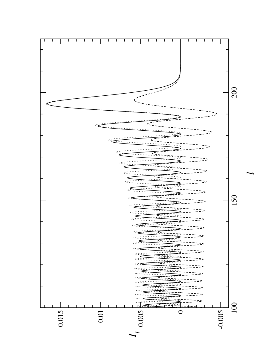
FIG. 1.:

REFERENCES

- [1] G. F. Smoot et al., Astrophys. J. 369, L1 (1992).
- [2] L. A. Page, astro-ph/9911199.
- [3] A. E. Lange et al., astro-ph/0005004.
- [4] S. Hanany et al., astro-ph/0005123.
- [5] G. Jungman, M. Kamionkowski, A. Kosowsky, and D. N. Spergel, Phys. Rev. D 54, 1332 (1996).
- [6] M. J. Rees, Astrophys. J. 153, L1 (1968).
- [7] J. R. Bond and G. Efstathiou, Astrophys. J. 285, L45 (1984).
- [8] M. Zaldarriaga, D. N. Spergel, and U. Seljak, Astrophys. J. 488, 1 (1997).
- [9] C. B. Netterfield et al., Astrophys. J. 474, L69 (1995).
- [10] S. T. Staggs, J. O. Gundersen, and S. E. Church, astro-ph/9904062.
- [11] M. White, J. E. Carlstrom, M. Dragovan, and W. L. Holzapfel, Astrophys. J. 514, 12 (1999).
- [12] See http://www.mrao.cam.ac.uk/telescopes/cat/vsa.html.
- [13] See http://astro.uchicago.edu/dasi/.
- [14] See http://astro.caltech.edu/tjp/CBI/.
- [15] See http://www.asiaa.sinica.edu.tw/amiba/.
- [16] H. M. Martin and R. B. Partridge, Astrophys. J. 324, 794 (1988).
- [17] P. T. Timbie and D. T. Wilkinson, Astrophys. J. 353, 140 (1990).
- [18] R. Subrahmanyan, R. D. Ekers, M. Sinclair, and J. Silk, Mon. Not. R. Astron. Soc. 263, 416 (1993).
- [19] M. P. Hobson, A. N. Lasenby, and M. Jones, Mon. Not. R. Astron. Soc. 275, 863 (1995).
- [20] M. P. Hobson and J. Magueijo, Mon. Not. R. Astron. Soc. 283, 1133 (1996).
- [21] R. Subrahmanyan, M. J. Kesteven, R. D. Ekers, M. Sinclair, and J. Silk, Mon. Not. R. Astron. Soc. 298, 1189 (1998).
- [22] M. White, J. E. Carlstrom, M. Dragovan, and W. L. Holzapfel, astro-ph/9912422.
- [23] M. Zaldarriaga and U. Seljak, Phys. Rev. D 55, 1830 (1997).
- [24] M. Kamionkowski, A. Kosowsky, and A. Stebbins, Phys. Rev. D 55, 7368 (1997).
- [25] K.-W. Ng and G.-C. Liu, Int. J. Mod. Phys. D 8, 61 (1999).
- [26] A. R. Thompson, J. M. Moran, and G. W. Swenson, Interferometry and Synthesis in Radio Astronomy (John Wiley & Sons, New York, 1986).
- [27] J. D. Kraus, Radio Astronomy, 2nd ed., Cygnus-Quasar Books (Powell, Ohio, 1986).
- [28] J. M. Wrobel and R. C. Walker, Lecture 9, Synthesis Imaging in Radio Astronomy II, edited by G. B. Taylor, C. L. Carilla, and R. A. Perley, ASP Conference Series Vol. 180 (Astronomical Society of the Pacific, California, 1999).
- [29] M. Abramowitz and I. A. Stegun, Handbook of Mathematical Functions (1964).
- [30] I. S. Gradshteyn and I. M. Ryzhik, Table of Integrals, Series, and Products (Academic Press, 1980).
- [31] L. Knox, Phys. Rev. D 52, 4307 (1995).
- [32] W. D. Cotton, Lecture 6 of Ref. [28].
- [33] E. Newman and R. Penrose, J. Math. Phys. 7, 863 (1966); J. N. Goldberg et al., ibid. 8, 2155 (1967).
- [34] R. Penrose and W. Rindler, Spinors and Space-time, Chapter 4 (Cambridge Univ. Press, 1984).