Reconnection in a striped pulsar wind

Abstract

It is generally thought that most of the spin-down power of a pulsar is carried away in an MHD wind dominated by Poynting flux. In the case of an oblique rotator, a significant part of this energy can be considered to be in a low-frequency wave, consisting of stripes of toroidal magnetic field of alternating polarity, propagating in a region around the equatorial plane. Magnetic reconnection in such a structure has been proposed as a mechanism for transforming the Poynting flux into particle energy in the pulsar wind. We have re-examined this process and conclude that the wind accelerates significantly in the course of reconnection. This dilates the timescale over which the reconnection process operates, so that the wind requires a much larger distance than was previously thought in order to convert the Poynting flux to particle flux. In the case of the Crab, the wind is still Poynting-dominated at the radius at which a standing shock is inferred from observation. An estimate of the radius of the termination shock for other pulsars implies that all except the milli-second pulsars have Poynting-flux dominated winds all the way out to the shock front.

1 Introduction

The diffuse synchrotron radiation from the Crab Nebula has now been observed in great detail in several wavebands, e.g., Hester et al. (1995). Although by far the best observed example, the Crab is just one of several pulsars surrounded by such a nebula (Arons, 1996), whose ultimate source of energy is almost certainly the rotational kinetic energy of the central neutron star (Pacini, 1967). However, despite intensive efforts, it is still not known how this energy is transferred from the neutron star to the radiating, relativistic electrons.

It is widely accepted that pulsars emit an electron-positron plasma, which carries away energy in the form of an ultra-relativistic magnetized wind, together with large amplitude waves (Rees & Gunn, 1974). At a shock front, located, in the case of the Crab Nebula, some $10^{17}\,$cm from the neutron star, this energy is released into the relativistic electrons responsible for the observed radiation. The most serious problem with this picture is that close to the strongly magnetized neutron star the energy must be carried mostly by electromagnetic fields as Poynting flux (Michel, 1982). But, in order to produce the radiating electrons, the energy flux at the shock front must be carried mainly by the particles (Rees & Gunn, 1974; Kennel & Coroniti, 1984; Emmering & Chevalier, 1987). As has been pointed out by several authors — and emphasized recently by Chiueh, Li & Begelman (1998) and Bogovalov & Tsinganos (1999) — in an ideal, ultra-relativistic MHD wind, there is no plausible way of converting the Poynting flux into particle energy flux. Several effects have been investigated in attempts to overcome this difficulty, ranging from rapid expansion in a magnetic nozzle (Chiueh, Li & Begelman, 1998) to non-ideal MHD effects in a two-fluid (electron and positron) plasma (Mestel & Shibata, 1994; Melatos & Melrose, 1996). It has also been suggested that a global non-axisymmetric instability of the nebular plasma alleviates the problem by enabling the conversion of magnetic to particle energy (Lyubarsky, 1992; Begelman, 1998). However, perhaps the most promising explanation to date has been that of reconnection in a striped pulsar wind, as advanced by Michel (1982), Coroniti (1990) and Michel (1994). Here, we reanalyze this process. Both Coroniti and Michel effectively assumed the wind maintained constant speed during reconnection. We find that the hot plasma in the current sheets where reconnection takes place performs work on the wind, accelerating it substantially. As a result, the reconnection rate is much slower than hitherto claimed. In the case of the Crab Nebula, we conclude that reconnection is not capable of converting a significant fraction of the energy flux before the wind reaches the position at which the shock front is encountered.

The conversion of Poynting flux to kinetic energy is also a central problem in a certain class of models of gamma-ray bursts. It has been proposed that the emission of a large amplitude electromagnetic wave by a black hole or neutron star(s) underlies the burst phenomenon, that the gamma-rays are generated by dissipative processes in the wave, and that the X-ray and lower frequency emission is produced at an outer shock front (Usov, 1992, 1994; Blackman & Yi, 1998). The calculations we present can be rescaled to this situation and may offer a mechanism for accelerating the wind to the very high Lorentz factors required before dissipation sets in.

The paper is organized as follows: in Section 2 we describe the problem as formulated by Coroniti (1990) and Michel (1994), present estimates of the effect of reconnection and explain in physical terms the reasons for our new result. The perturbation method we employ is a short wavelength approximation, which uses as a small parameter the ratio of the radius of the light cylinder to the actual radius. This is presented in outline in Section 3, relegating most of the algebra to the Appendix, but pointing out the differences between our method and that of Coroniti (1990). An analytic asymptotic solution to the system is given in Section 4, followed by results of a numerical integration of the equations and a discussion of the limitations of our approach. Finally, in Section 5, we summarize our conclusions and their implications, especially for our understanding of the Crab Nebula.

2 The striped wind

Despite the presence of a plasma, the total power lost by a rotating magnetized neutron star may be estimated using the formula for a magnetic dipole rotating in vacuum Gunn & Ostriker (1969), Michel (1982). However, the presence of plasma changes the physical picture significantly: for example, even an axisymmetric rotator surrounded by plasma loses energy by driving a plasma wind, in contrast to an aligned magnetic dipole in vacuum. Furthermore, although a strong vacuum electromagnetic wave readily loses energy to particles (Ostriker & Gunn, 1969; Asseo, Kennel & Pellat, 1978; Melatos & Melrose, 1996), the presence of plasma is likely to prevent the formation of such waves and restrict dissipation to shock fronts or regions in which the magnetic field undergoes reconnection.

In the case of an oblique rotator, the energy lost in the wind can be regarded as shared between an axisymmetric component of the Poynting flux and one due to MHD waves, the ratio being determined by the angle between the magnetic and rotational axes. Michel (1971) pointed out that such waves, which have a phase speed less than that of light, should evolve into regions of cold magnetically dominated plasma separated by very narrow, hot, current sheets. The formation of this pattern may be imagined as follows: in the axisymmetric case, a current sheet separates the two hemispheres with opposite polarity beyond the light cylinder. As the obliquity increases, this sheet begins to oscillate about the equatorial plane because the field line at a given radius alternates in direction with the frequency of rotation, being connected to a different magnetic pole every half-period. Such a picture is observed in Solar Wind. In a quasi-radial flow, the amplitude of these oscillations grows linearly with radius and at large distances one can locally imagine quasi-spherical current sheets following each another and separating the stripes of magnetized plasma with opposite polarity. Coroniti (1990) called this picture a striped wind. Recently Bogovalov (1999) has found an exact solution for the oblique split monopole case which has precisely this structure.

It was noticed by Usov (1975) and Michel (1982) that these waves must decay at large distances, since the current required to sustain them falls off as $r^{-1}$. This is slower than the fall-off in the available number of charge carriers, which goes as $r^{-2}$. Coroniti (1990) considered the reconnection process in a striped wind and came to the same conclusion. In the case of a highly oblique rotator, both Coroniti and Michel agreed that the MHD wind of the Crab pulsar could be transformed by this mechanism from one dominated by Poynting flux to one dominated by particle kinetic energy flux well within the radius of the termination shock.

The pulsar wind beyond the light cylinder is quasi-spherical (Chiueh, Li & Begelman, 1998; Bogovalov & Tsinganos, 1999), and, as the magnetic field is predominantly toroidal, it scales roughly as

$$B = B_{\rm L}\frac{r_{\rm L}}{r},$$ (1)

where $r_{\rm L}=c/\Omega=cP/2\pi$ is the light-cylinder radius, $\Omega$ the angular velocity of the neutron star $P$ its period of rotation and $B_{\rm L}$ the magnetic field strength at $r_{\rm L}$. Near the light cylinder, the poloidal and toroidal components are comparable, but within it the poloidal field is nearly dipolar, so that one can estimate

$$B_{\rm L} = \frac{\mu}{r_{\rm L}^{3}}\,\approx\,9\frac{\mu_{30}}{P^{3}}{\rm G},$$ (2)

where $\mu=10^{30}\mu_{30}\,$G$\cdot$cm³ is the magnetic moment of the star and $P$ is given in seconds. The density $n$ in the quasi-spherical flow, measured in the rest frame of the star, decreases approximately as

$$n = n_{\rm L}\left(\frac{r_{\rm L}}{r}\right)^{2},$$ (3)

since in a steady, spherical, relativistic flow $r^{2}nv$ is constant and the speed $v$ is close to $c$. The density is conveniently normalized by the Goldreich-Julian charge density $\rho_{\rm GJ}$:

$$n_{\rm L} = \kappa\rho_{\rm GJ}/e$$ (4)

$$= \frac{\kappa B_{\rm L}\Omega}{2\pi ec}$$

where $\kappa$ is the multiplicity coefficient. This quantity is rather uncertain but generally expected to be large: $\kappa\sim 10^{3}-10^{4}$ (Arons, 1983).

The Poynting flux may be estimated as

$$W = \frac{cB_{\rm L}^{2}}{4\pi}\left(\frac{r_{\rm L}}{r}\right)^{2}$$ (5)

and the ratio of the Poynting flux to the kinetic energy flux, called the magnetization parameter $\sigma$, is

$$\sigma = \frac{W}{mc^{3}\gamma n}\enspace.$$ (6)

At the light cylinder this quantity takes on the value

$$\sigma_{\rm L} = {\omega_{\rm L}\over 2\gamma_{\rm L}\kappa\Omega}$$ (7)

$$= 1\cdot 3\times 10^{7}{\mu_{30}\over\gamma_{\rm L}\kappa P^{2}}$$ (8)

where $\omega_{\rm L}=eB_{\rm L}/mc$ is the gyrofrequency at the light cylinder. The ratio $\omega_{\rm L}/\Omega$ is large for all pulsars. For example, in the case of the Crab, where $\mu_{30}\approx 5$, we have $\omega_{\rm L}/\Omega\approx 10^{11}$.

The speed of a fast magnetosonic wave propagating perpendicular to the magnetic field in a magnetically dominated plasma corresponds to a Lorentz factor $\gamma_{\rm fms}=\sqrt{\sigma}$ [e.g., Kirk & Duffy (1999)]. In pulsar models, plasma is ejected at Lorentz factors of $10^{2}$ to $10^{3}$, which is higher than $\gamma_{\rm mfs}$ for most pulsars. In the case of the Crab, however, these values correspond to a trans-alfvénic speed ($\gamma_{\rm L}\sim\sqrt{\sigma_{\rm L}}$) at the light cylinder. At some point beyond the light cylinder, but before the onset of dissipation, we expect the wind to establish a supersonic ideal MHD flow, in which the value of $\sigma$ and $\gamma$ are constant. In the following, these values are indicated by the subscript ‘L’, even though, strictly speaking, they may not be achieved at the light cylinder itself. Using the above estimates, we then find that, for the Crab, $\kappa=10^{4}$ corresponds to $\sigma_{\rm L}\approx 3\times 10^{4}$ and $\gamma_{\rm L}\approx 200$. At the light cylinder, almost all the energy is carried by the electromagnetic field. If this energy were completely transferred from Poynting flux into plasma kinetic energy, the Lorentz factor would attain the value

$$\gamma_{\rm max} = \gamma_{\rm L}\sigma_{\rm L}$$ (9)

$$= \frac{\omega_{\rm L}}{2\kappa\Omega}.$$

However, a cold, radial MHD wind does not accelerate, because the outwardly directed pressure gradient arising from the gradient of the magnetic field is exactly balanced by the inwardly directed tension force exerted by the curved toroidal field lines. In the absence of dissipation, the energy flux remains locked in the field as Poynting flux.

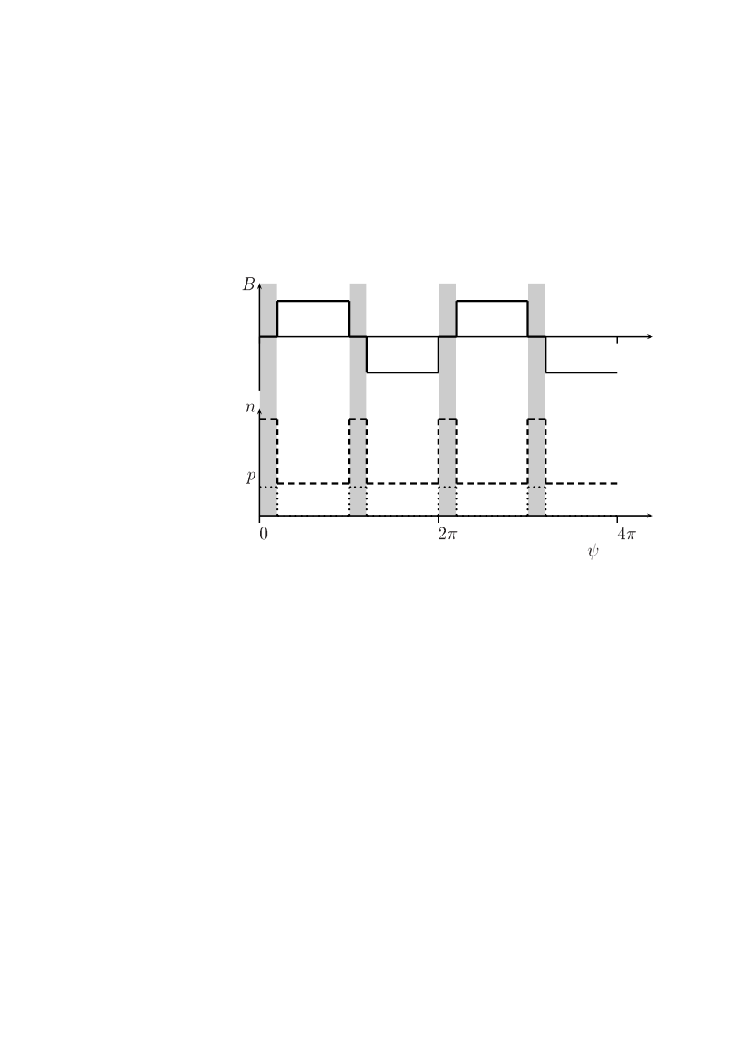
Figure 1: Idealized picture of a pulsar wind driven by a rotating, perpendicular, split-monopole magnetic field, showing the magnetic field, $B$ (solid line), particle density $n$ (dashed line) and plasma pressure $p$ (dotted line) as functions of the phase variable $\phi=r/r_{\rm L}$, with origin at an arbitrary position in the outer part of the wind ($r\gg r_{\rm L}$). The magnetic field and density are constant between the current sheets, which are shown shaded. Within the sheets, we assume zero magnetic field and constant density.

The idealized radial structure of the wind and embedded current sheets corresponding to the field of a perpendicular split monopole is shown in Fig. 1. In the proper plasma frame the current density $I^{\prime}$ (current per unit length in the toroidal direction) is, according to Ampère’s law,

$$I^{\prime} = \frac{cB^{\prime}}{2\pi}.$$ (10)

Here and in the following we use primed values to indicate quantities in the proper plasma frame, e.g., $B^{\prime}=B/\gamma$, $n^{\prime}=n/\gamma$ etc. Usov (1975) and Michel (1982) noticed that the current in Eq. (10) cannot be maintained to arbitrarily large radius: since the proper current density cannot exceed $en^{\prime}c$ and the width of the sheet is less than half a wavelength, $\pi r_{\rm L}$, one can easily see from Eqs.(1), (3) and (4) that the striped wind cannot exist beyond the radius

$$r_{\rm max} = \pi\kappa\gamma r_{\rm L}$$ (11)

[see also (Melatos & Melrose, 1996)]. When the velocity of the current carriers approaches the speed of light, an anomalous resistance arises and the alternating magnetic field dissipates by heating the plasma. Coroniti (1990) considered the dissipation as reconnection through the current sheet, whose minimum thickness he took equal to the Larmor radius which a thermal particle of the hot plasma in the sheet would have, if it entered the cold magnetized part of the wind. In terms of the fraction $\Delta$ of a wavelength $2\pi r_{\rm L}$ occupied by the two current sheets, this condition reads

$$\Delta > {T^{\prime}\over\pi\gamma r_{\rm L}eB^{\prime}}$$ (12)

where $T^{\prime}$ is the characteristic “temperature” of the particles in the sheet, in energy units. Taking into account that the sheet is in pressure equilibrium,

$$n^{\prime}T^{\prime} = {B^{\prime 2}\over 8\pi}$$ (13)

one can easily see that the current density $j^{\prime}<en^{\prime}c$, so that Coroniti’s condition is, to within a factor of the order of unity, the same as that of Michel (1994).

If, initially, a fraction $\alpha$ of the plasma is concentrated in the sheets, dissipation begins at a radius $r_{1}=\alpha r_{\rm max}$. For $r<r_{1}$ the sheet width exceeds the limiting value of Eq. (12), the current carriers remain non-relativistic, the conductivity is very high and reconnection does not proceed. For $r>r_{1}$, however, the current carriers become relativistic, an anomalous resistivity arises, and reconnection brings energy and plasma into the sheet until, eventually, all the magnetic flux is destroyed at the radius $r=r_{\rm max}$.

Both Michel and Coroniti estimated the radius $r_{\rm max}$ by substituting into Eq.(11) the initial Lorentz factor $\gamma_{\rm L}$. The corresponding value is large compared to the light cylinder radius. For the Crab, it is of the order of $10^{7}r_{\rm L}$, which is, nevertheless, still well within the radius of the standing shock $r_{\rm s}\approx 10^{9}r_{\rm L}$. However, as we show below, the flow accelerates as reconnection proceeds. Basically, this is because the hot plasma continues to exert an outwardly directed pressure gradient, but the compensating inwardly directed tension force is absent. Equivalently, it is clear that the hot plasma performs work during the radial expansion, and this appears as an acceleration of the wind. In an accelerating wind, most of the energy is released when the Lorentz factor of the flow is roughly at its maximum value, given by Eq. (9). The corresponding radius is

$$r_{\rm max} = \pi\kappa\gamma_{\rm max}r_{\rm L}$$

$$= \frac{\pi\omega_{\rm L}}{2\Omega}r_{\rm L}$$

$$= 2\cdot 10^{17}\frac{\mu_{30}}{P}\,{\rm cm}$$

In the case of the Crab, $r_{\rm max}\approx 10^{11}r_{\rm L}$, which significantly exceeds the radius of the standing shock, so that only a small fraction of the wave energy is converted into particle energy before the plasma arrives at this shock front.

3 Equations

3.1 Local structure of the wave

The striped wind described above can be regarded as an MHD wind containing an entropy wave which moves together with the plasma. At large distances the wave consists locally of spherical current sheets separating cold, magnetized stripes of plasma with opposing polarity (see Fig. 1). To find the evolution of this wave, we use a two-timescale perturbation approach, assuming that the timescale on which it evolves i.e., the timescale on which the reconnection sheet grows, is much longer than the period $P$ of the wave. Details of this method are presented in the Appendix. Here we restrict ourselves to the most important steps in the argument.

In the cold magnetized part of the wind the magnetic field $B$, which is toroidal, is constant on the fast timescale and the plasma pressure vanishes. The plasma density $n^{\prime}_{\rm c}$ ($n_{\rm c}$ in the lab. frame) is also constant on the fast timescale. In the hot sheet, the magnetic field vanishes, the pressure $p^{\prime}$ is constant on the fast timescale, as is the plasma density $n^{\prime}_{\rm h}$, which, in contrast to previous treatments, is not constrained to equal $n^{\prime}_{\rm c}$. In the plasma frame the entire pattern is at rest, but the plasma speed $v$, and the corresponding Lorentz factor $\gamma$ change on the slow timescale as the wave evolves. In the cold part of the wind, the magnetic field is frozen into the plasma, so that in spherical polar coordinates we can write for the slow evolution in radius

$${{\rm d}\over{\rm d}r}\left({B\over rn_{\rm c}}\right) = 0.$$ (15)

[see Eq. (A33)]. Although the method is strictly valid only for $r\gg r_{\rm L}$, we normalize the quantities in the wind to their value at $r=r_{\rm L}$. Using Eq. (4) and interpreting the multiplicity factor as referring to the density of electron/positron pairs outside the current sheets, this yields

$${B^{\prime}\over rn^{\prime}_{\rm c}} = {2\pi e\over\kappa}.$$ (16)

Following Coroniti (1990), we assume that reconnection keeps the sheet width equal to the limiting value given in Eq. (12) and (A32). The condition that the cold and hot parts of the flow are in pressure equilibrium (13) leads, together with Eq. (16), to the relation

$$\Delta = {rZc\over 4\pi\gamma vr_{\rm L}\kappa}$$ (17)

where a useful variable

$$Z = {n^{\prime}_{\rm c}\over n^{\prime}_{\rm h}}\,=\,{n_{\rm c}\over n_{\rm h}}$$ (18)

has been introduced. In his treatment, Coroniti (1990) set $n^{\prime}_{\rm h}=n^{\prime}_{\rm c}$ to write his equation (16) — the counterpart of our Eq. (17).

The remaining equations needed to describe the wave evolution are those of conservation of particle number and energy (equivalent to the equation of motion in the relativistic formulation) and the entropy equation. To zeroth order in $r_{\rm L}/r$ these confirm that the plasma speed equals the pattern speed, the hot and cold parts are in pressure equilibrium and the configuration shown in Fig. 1 and described above is stationary on the fast timescale.

3.2 The continuity equation

The slow evolution of the system is obtained by averaging over a wave-period, which we denote by angle brackets: $\left<\dots\right>$. Conservation of particle number (the continuity equation) gives

$$\left<nvr^{2}\right> = {\rm constant}$$ (19)

This equation is exact. In the short wavelength approximation, one can replace the time average by a spatial one, because all slowly varying parameters are constants on the scale of one wavelength. This immediately yields

$$vr^{2}n_{\rm c}\left[{\Delta\over Z}+\left(1-\Delta\right)\right] \equiv C_{1}\,=\,{\rm constant}$$ (20)

[see Eq. (A34), noting that in this section we use $\gamma$ and $v$ to refer to the zeroth order quantities, denoted in the Appendix by $\gamma_{0}$ and $v_{0}$].

3.3 The energy equation

After time averaging, the energy equation is

$$r^{2}\left<w^{\prime}\gamma^{2}v+\frac{EB}{4\pi}c\right> = {\rm constant}$$ (21)

Here $w^{\prime}$ is the enthalpy density: outside of the sheets $w^{\prime}=mn^{\prime}_{\rm c}c^{2}$, whereas within them $w^{\prime}=4p^{\prime}+mn^{\prime}_{\rm h}c^{2}$ ($=B^{\prime 2}/2\pi+mn^{\prime}_{\rm h}c^{2}$). One can substitute for the electric field using $E=vB$ because, by assumption, $E$ and $B$ are nonzero only outside the sheets, where magnetic field is frozen into the plasma.

Replacing once again in Eq. (21) the time average by a spatial one yields

$$\gamma^{2}vr^{2}\left[\left(\frac{B^{\prime 2}}{2\pi}+{mn^{\prime}_{\rm c}c^{2}\over Z}\right)\Delta+(1-\Delta)\left(mn^{\prime}_{\rm c}c^{2}+\frac{B^{\prime 2}}{4\pi}\right)\right] \equiv C_{2}\,=\,{\rm constant}$$ (22)

[see Eq. (A35)].

Coroniti (1990) did not use equation (21) in his analysis. Instead, he assumed the plasma both inside and outside of the sheet is strictly stationary in the wave frame so that the sheet edge moved through a constant density plasma. This led him to set $n^{\prime}_{\rm h}=n^{\prime}_{\rm c}$ in Eq. (17) (our numbering), thus reducing the number of unknowns. He was then able to find an expression for the speed of the sheet edge. However, such a picture violates energy conservation, as is apparent from Eq. (21): the condition of pressure equilibrium ($p^{\prime}=B^{2}/8\pi\gamma^{2}$) means that a decrease in the enthalpy flux in the magnetized part of the flow ($=r^{2}vB^{2}/4\pi$) cannot be balanced by an increase in the enthalpy flux in the sheet ($=r^{2}w^{\prime}\gamma^{2}v=4r^{2}p^{\prime}\gamma^{2}v$) unless there is a velocity (and density) jump across the sheet edge.

3.4 The entropy equation

The entropy equation requires more care. Following Eq. (21) of Coroniti (1990) and setting the ratio of specific heats to $4/3$, we write for the full nonlinear equation:

$$3{{\rm d}p^{\prime}\over{\rm d}t}-4{p^{\prime}\over n^{\prime}}{{\rm d}n^{\prime}\over{\rm d}t} = \left(E-{v\over c}B\right)j$$ (23)

(see Eq. A4) where the convective derivative $d/dt\equiv\partial/\partial t+v\partial/\partial r$. The right-hand side of this equation, when multiplied by $\gamma$, is the rate of entropy generation in the rest-frame of the plasma, which moves with speed $v$. In the limit of a sharp transition between the magnetized and unmagnetized parts of the flow, the entropy generation term is the product of two singular functions: one for the current and another for the electric field in the plasma frame. To find the slow evolution of the wave, it is essential to perform the averaging process before inserting this specific representation, which is not well-defined at the point at which entropy is generated. In moving from his Eq. (21) to (22), Coroniti overlooked this point. As a consequence of this, and of the incorrect expression for the expansion speed of the sheets, he came to the erroneous conclusion [in his equation (26)] that the wave Lorentz factor remains almost constant during reconnection.

Following the averaging procedure described in the Appendix (Eqs. A27 to A30), we find [see Eq. (A37)]:

$${4p^{\prime}\over r^{2}}{\partial\over\partial r}\left(r^{2}\gamma v\Delta\right)+3\gamma v{\partial\over\partial r}\left(\Delta p^{\prime}\right)+$$

$${v\over\gamma}{\partial\over\partial r}\left[\gamma^{2}\left(1-\Delta\right)p^{\prime}\right]+{2\gamma p^{\prime}\left(1-\Delta\right)\over r}{\partial\over\partial r}\left(rv\right) = 0\enspace.$$ (24)

This equation may be integrated, using the equations of continuity (20) and flux freezing (16):

$$(1-3Z)n^{\prime}_{\rm c}r^{3} \equiv C_{3}\,=\,{\rm constant}$$ (25)

[See Eqs. (A38–A42)].

The system thus consists of five algebraic equations (16), (17), (20), (22) and (25) for the five slowly varying unknown functions of radius: $n^{\prime}_{\rm c}$, $Z$, $B^{\prime}$, $\Delta$ and $\gamma$.

4 Results

4.1 Asymptotic solution

A general solution to this system is difficult to find, and the most straightforward way to generate a numerical solution is to revert to integrating the differential forms of the continuity, energy and entropy equations. However, it is possible to extract analytically an asymptotic solution, valid for $\Delta$, $\gamma^{-2}$, $\sigma_{\rm L}^{-1}\ll 1$, which is just the regime we are interested in.

As can be checked a posteriori, the quantity $n^{\prime}_{\rm c}r^{3}$ is an increasing function of $r$, so that, according to Eq. (25), $Z\rightarrow 1/3$ as $r\rightarrow\infty$. Defining, in accordance with Eq. (7),

$$\sigma_{\rm L} = \left[{B^{\prime 2}/4\pi\over mn^{\prime}_{\rm c}c^{2}}\right]_{r=r_{\rm L}}$$ (26)

we can use the continuity equation (20) to rewrite the energy equation (22) as

$$\gamma^{2}vr^{2}(1+\Delta){B^{\prime 2}\over 4\pi}+\gamma mc^{2}C_{1} = \gamma_{\rm L}mc^{2}C_{1}(1+\sigma_{\rm L})\enspace.$$ (27)

Here we have assumed the initial thickness of the current sheet is vanishingly small. This is reasonable, since before the onset of reconnection, the plasma in the sheet expands adiabatically and cools, causing the sheet width to decrease. To lowest order in the small parameters, this equation (27), together with Eq. (16), and the continuity equation (20) yield the same result:

$$\gamma r^{2}n^{\prime}_{\rm c} = C_{1}$$ (28)

so that the system is nearly degenerate. Expanding the equations to next order and eliminating the leading term gives

$$\sigma_{\rm L}\left({2\Delta\over Z}-3\Delta+{1\over 2\gamma_{\rm L}^{2}}-{1\over 2\gamma^{2}}\right) = {\gamma\over\gamma_{\rm L}}-1\enspace.$$ (29)

At large radius $Z\rightarrow 1/3$ and for a super-Alfvénic flow ($\gamma\gg\gamma_{\rm L}>\sqrt{\sigma}$), one finds $\gamma/\gamma_{\rm L}\rightarrow 3\sigma_{\rm L}\Delta$, leading to the asymptotic solution

$$\gamma = \sigma_{\rm L}\gamma_{\rm L}\left[{\Omega r\over 2\pi\omega_{\rm L}r_{\rm L}}\right]^{1/2}$$ (30)

$$\Delta = \left[{\Omega r\over 18\pi\omega_{\rm L}r_{\rm L}}\right]^{1/2}$$ (31)

$${T^{\prime}\over mc^{2}} = {\sigma_{\rm L}\gamma_{\rm L}\over 6\gamma}\,=\,\left[{18\Omega r\over\pi\omega_{\rm L}r_{\rm L}}\right]^{-1/2}$$ (32)

$$p^{\prime} = \left({B_{\rm L}^{2}\over 8\pi\gamma_{\rm L}^{2}}\right)\left({r\over r_{\rm L}}\right)^{-3}{2\pi\omega_{\rm L}\over\Omega}$$ (33)

which agrees with our estimate that the maximum value of $\gamma$ given in Eq. (9) is attained at the radius $r_{\rm max}$ of Eq. (2), where $\Delta\sim 1$. Note that this solution is independent of the actual value of $\gamma_{\rm L}$, which enters only as a scaling factor for $\gamma$.

4.2 Numerical solution

Figure 2: Results of a numerical integration the system of equations (A34), (A35) and (A37) for three different initial conditions, superposed on the analytic asymptotic solution (dashed line). The parameters used are those appropriate for the Crab: $\sigma_{\rm L}=3\times 10^{4}$, $\gamma_{\rm L}=200$, $\omega_{\rm L}/\Omega=10^{11}$. Plotted are the temperature $T$ in the hot sheet, in units of $mc^{2}$, the fraction $\alpha$ of particles in the sheet [$\Delta n^{\prime}_{\rm h}/[\Delta n^{\prime}_{\rm h}+(1-\Delta)n^{\prime}_{\rm c}]$] the Lorentz factor of the flow $\gamma$ and the fraction of a wavelength occupied by the sheets $\Delta$, as functions of the radius in units of the light cylinder radius. The initial conditions correspond to reconnection starting at $r/r_{\rm L}=10$ (solid line), $10^{3}$ (dotted line) and $10^{5}$ (dashed-dotted line). In the Crab, the termination shock is located at $\log(r/r_{\rm L})\approx 9$.

Three physical parameters determine the cold radial MHD wind of a pulsar in the absence of reconnection. They are the values at the light cylinder of the magnetization parameter $\sigma_{\rm L}$, Lorentz factor $\gamma_{\rm L}$ and the ratio of the particle gyro frequency to the rotation period $\omega_{\rm L}/\Omega$. These are related to the multiplicity parameter $\kappa$ by Eq. (7). In the presence of reconnection, the same three parameters also uniquely specify the asymptotic solution at large radius Eqs. (30–33). However, the full solution requires one additional initial condition, which is the fraction $\alpha$ of plasma which is initially present in the current sheets. This quantity determines the radius at which reconnection starts, which is, formally, the position at which we impose the initial condition $\Delta=0$. The perturbation analysis presented above is valid when this radius is large compared to $r_{\rm L}$.

To investigate the dependence of the solutions on this initial condition, we have solved the system by integrating numerically the three equations continuity, energy and entropy written in differential form: (A34), (A35) and (A37). The results are shown in Fig. 2, for parameters appropriate for the Crab pulsar: $\sigma_{\rm L}=3\times 10^{4}$, $\gamma_{\rm L}=200$, ($>\sqrt{\sigma_{\rm L}}$, so that the wind is initially supersonic) and $\omega_{\rm L}/\Omega=10^{11}$. The multiplicity parameter for these parameters is $\kappa=8\times 10^{3}$. Solutions for three different initial conditions are shown, corresponding to starting points for reconnection at $10$, $10^{3}$ and $10^{5}\times r_{\rm L}$. Superposed on these solutions is the analytic asymptotic solution. For all values of the initial condition, the asymptotic solution is approached rapidly, and followed closely, until $\Delta\sim 1$. The termination shock in the wind of the Crab pulsar is thought to lie at roughly $r_{\rm s}\approx 10^{9}r_{\rm L}$. At this point, $\Delta\sim 0.01$ and the energy flux is still dominated by Poynting flux.

4.3 Validity of the solutions

The range of validity of our treatment is limited by two factors. According to our solutions, the temperature in the current sheets decreases outward. The expression used for the gyro-radius in Eqs. (17) and (A32) assumes $T>mc^{2}$, as does the choice $\hat{\gamma}=4/3$ for the ratio of specific heats. This is not the case at very large radius and the range of validity is therefore restricted to

$$\gamma < {\gamma_{\rm max}\over 6}$$ (34)

At the upper end of this range, $\Delta=1/18$, so the assumption $\Delta\ll 1$ is still valid. The corresponding radius $r_{2}$ is

$$r_{2} = \frac{\pi\omega_{\rm L}}{18\Omega}r_{\rm L}=\frac{10^{6}\mu_{30}}{P^{2}}r_{\rm L}$$ (35)

At this point, the fraction of the Poynting flux transferred to the plasma is still small. For the Crab, one obtains (see Fig. 2) $r_{2}\approx 10^{10}r_{\rm L}$, which already exceeds the radius of the standing shock. Thus, our treatment is valid up to the shock front, before which reconnection is indeed ineffective in the wind of this pulsar.

The second limitation concerns the assumption that the dissipation proceeds sufficiently quickly to keep the sheet thickness equal to the minimum value given by Eq. (12). This assumption holds provided the proper propagation time, $r/(c\gamma)$, exceeds the Larmor period. Because the sheet width is equal to the Larmor radius, this condition,

$$\frac{r}{\gamma} > 4\pi^{2}\Delta\gamma r_{\rm L}$$ (36)

is equivalent, to within a factor of the order of unity, to the condition that pressure equilibrium within the sheet has time to be established. Substituting Eq. (31) and $Z=1/3$, one finds

$$\gamma < \gamma_{\rm M}\,=\,3\kappa.$$ (37)

If $\gamma_{\rm max}>\gamma_{\rm M}$, the flow accelerates only up to the point where $\gamma=\gamma_{\rm M}$, after which no further dissipation can occur. This regime arises for

$$\kappa < \sqrt{\omega_{\rm L}\over 6\Omega}$$ (38)

$$= 2\cdot 10^{3}{\sqrt{\mu_{30}}\over P}$$ (39)

or, alternatively,

$$\gamma_{\rm max} = \sigma_{\rm L}\gamma_{\rm L}\,>\,\sqrt{3\omega_{\rm L}\over 2\Omega}$$ (40)

$$= 6\cdot 10^{3}{\sqrt{\mu_{30}}\over P}$$ (41)

Otherwise, acceleration continues and the flow can, in principle, reach $\gamma_{\rm max}$, unless it encounters a shock front.

In the case of a pulsar moving through the interstellar medium, one can estimate the position of the termination shock by equating the magnetic pressure to the ram pressure of the medium:

$${B_{\rm L}^{2}\over 8\pi}\left({r_{\rm L}\over r}\right)^{2} = \rho V^{2}$$ (42)

where $\rho$ is the density of the interstellar medium, and $V$ the velocity of the pulsar through it. Taking $V=100\,{\rm km\,s}^{-1}$ and a particle density of $1\,{\rm cm}^{-3}$, one obtains

$$r_{\rm s} = 7\times 10^{14}{\mu_{30}\over P^{2}}\,{\rm cm}\enspace.$$ (43)

Comparing this with the expression for $r_{\rm max}$, Eq. (2), one sees that the flow remains Poynting dominated up to the termination shock for all but the milli-second pulsars.

5 Conclusions

We have examined the fate of a wave generated in a pulsar wind by the rotating, magnetized neutron star. This wave is built from the oscillating equatorial current sheet which, at large distances, may be considered locally as a sequence of spherical current sheets separated in radius by the distance $\pi r_{\rm L}$. As was suggested by Usov (1975) and Michel (1982), the wave decays because the particle number density eventually becomes insufficient to maintain the necessary current. Dissipation begins when the velocity of the current carriers reaches the speed of light or, almost equivalently, when the sheet width becomes equal to the Larmor radius (Coroniti, 1990; Michel, 1994). The dissipation process may be considered as reconnection of oppositely directed magnetic fields (Coroniti, 1990). In the proper plasma frame, plasma from the inter sheet space slowly moves towards the sheet, which slowly expands, absorbing more plasma and magnetic energy. The distance at which the wave decays completely is proportional to the Lorentz-factor $\gamma$ of the flow [Eq.(9)], as found by Michel and Coroniti. In this formula, however, they inserted the initial Lorentz-factor, $\gamma\sim 100-1000$ and concluded that in the case of the Crab pulsar the wave decays well before the wind reaches the termination shock.

We find that the flow accelerates during the dissipation process. The reason is that in the freely expanding flow, hot plasma in the current sheet performs work on the flow. The restraining magnetic tension force is released by reconnection, but the accelerating pressure gradient remains. As a result, most of the magnetic energy is dissipated when the flow has accelerated to a Lorentz-factor which is of the same order as the maximal one. For the Crab, the corresponding distance is well beyond the standing shock, so we conclude that the wave does not dissipate before entering the shock. Using a simple estimate of the location of the termination shock for other isolated pulsars, we find this conclusion holds for all except those of milli-second period. In the Appendix, we show that our result applies not only to the singular current sheet structure discussed by Coroniti (1990), but also to a more general smooth distribution of current and magnetic field.

Exactly how the wind energy dissipates remains a mystery, not only in the case of pulsars, but also in the closely related models proposed for gamma-ray bursts (Usov, 1992, 1994; Blackman & Yi, 1998). At present, one can only speculate that dissipation might be possible in a combination of shocks and current sheets at the position of the bright equatorial X-ray torus observed in the Crab (Brinkmann, Aschenbach & Langmeier, 1985). If the Crab is an oblique rather than a perpendicular rotator, a significant part of the energy flux at high latitudes is transferred by the axisymmetric part of the Poynting flux, which cannot dissipate by reconnection. It has been suggested that the release of this energy may be triggered by the kink instability (Lyubarsky, 1992; Begelman, 1998), giving rise to the jet-like structure observed in the Crab Nebula, orientated, presumably, along the rotation axis of the pulsar (Hester et al., 1995). Thus, the idea that dissipation of the axisymmetric component and the wave component of the Poynting flux is fundamentally different has both observational and theoretical support. Current sheets are not expected to be responsible for the former. We have demonstrated in this paper that they also cannot be responsible for the latter, until the pulsar wind encounters the termination shock.

Appendix A Equations of entropy-wave evolution in the two-timescale approximation

A.1 MHD equations

Consider a non-steady, axially symmetric, radial MHD wind. In spherical coordinates, the electromagnetic fields, fluid velocity and current density in the laboratory frame are $\vec{B}=B(r,t){\bf\hat{\varphi}}$, $\vec{E}=E(r,t){\bf\hat{\theta}}$, $\vec{v}=v(r,t){\bf\hat{r}}$, $\vec{j}=j(r,t){\bf\hat{\theta}}$, and the proper (i.e., in the fluid rest frame) energy density, pressure, temperature (in energy units) and number density are $e^{\prime}(r,t)$, $p^{\prime}(r,t)$ $T^{\prime}(r,t)$ and $n^{\prime}(r,t)$.

Then the equations of MHD are that of continuity:

$${\partial\over\partial t}(\gamma n^{\prime})+{1\over r^{2}}{\partial\over\partial r}(r^{2}\gamma vn^{\prime}) = 0$$ (A1)

(where $\gamma=1/\sqrt{1-v^{2}/c^{2}}$), the energy equation (zeroth component of the divergence of the stress-energy tensor):

$${\partial\over\partial t}(T^{00})+{1\over r^{2}}{\partial\over\partial r}(r^{2}T^{01}) = 0$$ (A2)

where

$$T^{00} = (e^{\prime}+p^{\prime})\gamma^{2}-p^{\prime}+{E^{2}+B^{2}\over 8\pi}$$

$$T^{01} = (e^{\prime}+p^{\prime})\gamma^{2}v+{EBc\over 4\pi}$$ (A3)

the entropy equation:

$${1\over\hat{\gamma}-1}\left({{\rm d}p^{\prime}\over{\rm d}t}-{\hat{\gamma}p^{\prime}\over n^{\prime}}{{\rm d}n^{\prime}\over{\rm d}t}\right) = \left(E-{v\over c}B\right)j$$ (A4)

(where ${\rm d}/{\rm d}t\equiv\partial/\partial t+v\partial/\partial r$ and $\hat{\gamma}$ is the ratio of specific heats) and the two Maxwell equations

$${1\over r}{\partial\over\partial r}(rB)+{1\over c}{\partial E\over\partial t}+{4\pi\over c}j = 0$$ (A5)

(Ampère’s law) and

$${1\over r}{\partial\over\partial r}(rE)+{1\over c}{\partial B\over\partial t} = 0$$ (A6)

(Faraday’s law). The system is completed by Ohm’s law

$$j = \sigma_{\rm c}\gamma\left(E-{v\over c}B\right)$$ (A7)

the ideal gas law

$$p^{\prime} = n^{\prime}T^{\prime}$$ (A8)

and an equation of state, for which we select

$$p^{\prime} = (\hat{\gamma}-1)(e^{\prime}-n^{\prime}mc^{2})$$ (A9)

where $m$ is the (mean) particle rest mass. In the following we will take $\hat{\gamma}=4/3$, as appropriate for a relativistic gas.

Eliminating $n^{\prime}$ from Eq. (A4) using the equation of continuity (A1) we find

$$4p^{\prime}{\partial\gamma\over\partial t}+3\gamma{\partial p^{\prime}\over\partial t}+{4p^{\prime}\over r^{2}}{\partial\over\partial r}(r^{2}\gamma v)+3v\gamma{\partial p^{\prime}\over\partial r} = \gamma\left(E-{v\over c}B\right)j\enspace.$$ (A10)

In the limit of a relativistic gas, $e^{\prime}\rightarrow 3p^{\prime}$, the set of equations (A2), (A10), (A5) and (A6) is then independent of $n^{\prime}$, which appears only in the continuity equation (A1).

A.2 Perturbative solution

To solve these equations, we exploit the two-timescales present in the problem. The fast timescale is that of the pulsar rotation period $t_{\rm fast}=P\equiv 2\pi/\Omega$. We assume that the initial conditions in the wind close to the star have period $P$ and that at any fixed radius, all quantities vary with this period. At a distance of a few light-cylinder radii ($r_{\rm L}\equiv c/\Omega$), we assume that the wind has settled down into an almost stationary pattern in which the fluid speed does not vary on the fast timescale, although the density, pressure and especially the magnetic field do so. Our initial conditions at this distance, therefore, constitute an entropy wave comoving with the fluid. The wave evolves on the slow timescale which is the expansion timescale of the wind $t_{\rm slow}\sim rP/r_{\rm L}$. For $r\gg r_{\rm L}$, we have conditions suitable for a two-timescale expansion, i.e., $t_{\rm fast}\ll t_{\rm slow}$. The general procedure is: i) transform to fast and slow independent variables, ii) expand the dependent variables, iii) collect and solve the zeroth order equations, and iv) collect the first order equations and demand that the secular terms they contain vanish (Nayfeh, 1973).

First, we define a fast phase variable

$$\phi = \Omega\left[t-\int_{0}^{r}{{\rm d}r^{\prime}\over v_{\rm w}(r^{\prime})}\right]$$ (A11)

where $v_{\rm w}(r)$ is the speed of the pattern, which is to be determined. We now change variables from $(r,t)$ to $(\phi,R)$, where the dimensionless ‘slow’ variable is defined as

$$R = \varepsilon r/r_{\rm L}$$ (A12)

with $\varepsilon\ll 1$ and $R\sim 1$. In terms of the new variables, we find for the continuity equation (A1):

$${\partial\over\partial\phi}(\gamma n^{\prime})-{1\over v_{\rm w}}{\partial\over\partial\phi}(\gamma vn^{\prime})+{\varepsilon\over R^{2}}{\partial\over\partial R}(R^{2}\gamma vn^{\prime}) = 0$$ (A13)

the energy equation (A2):

$${\partial T^{00}\over\partial\phi}-{1\over v_{\rm w}}{\partial T^{01}\over\partial\phi}+{\varepsilon\over R^{2}}{\partial\over\partial R}(R^{2}T^{01}) = 0$$ (A14)

the modified entropy equation (A10):

$$4p^{\prime}{\partial\gamma\over\partial\phi}+3\gamma{\partial p^{\prime}\over\partial\phi}-4{p^{\prime}\over v_{\rm w}}{\partial\over\partial\phi}(\gamma v)-$$ (A15)

$$3{\gamma v\over v_{\rm w}}{\partial p^{\prime}\over\partial\phi}+{4\varepsilon p^{\prime}\over R^{2}}{\partial\over\partial R}(R^{2}\gamma v)+3\varepsilon\gamma v{\partial p^{\prime}\over\partial R}\,=\,{1\over\Omega}\gamma(E-vB)j$$

Ampère’s equation (A5):

$${\partial E\over\partial\phi}-{1\over v_{\rm w}}{\partial B\over\partial\phi}+{\varepsilon\over R}{\partial\over\partial R}(RB)+{4\pi\over\Omega}j = 0$$ (A16)

Faraday’s equation (A6):

$${\partial B\over\partial\phi}-{1\over v_{\rm w}}{\partial E\over\partial\phi}+{\varepsilon\over R}{\partial\over\partial R}(RE) = 0\enspace.$$ (A17)

In these equations we have expressed all velocities in units of the speed of light ($v\rightarrow cv$ etc.).

We now expand the dependent variables, noting that for an entropy wave the zeroth order velocity is independent of the phase:

$$v = v_{0}(R)+\varepsilon v_{1}(\phi,R)$$

$$n^{\prime} = n^{\prime}_{0}(\phi,R)+\varepsilon n^{\prime}_{1}(\phi,R)$$

$$p^{\prime} = p^{\prime}_{0}(\phi,R)+\varepsilon p^{\prime}_{1}(\phi,R)$$ (A18)

etc.

Substituting and collecting terms of order $\varepsilon^{0}$ we find from the continuity equation (A13) that for a non-uniform wind (one in which $\gamma_{0}n_{0}$ is a function of $\phi$)

$$v_{\rm w} = v_{0}(R)\enspace.$$ (A19)

The Maxwell equations (A17) and (A16) then lead to

$${\partial B_{0}\over\partial\phi} = {4\pi\gamma_{0}^{2}v_{0}\over\Omega}j_{0}\enspace.$$ (A20)

From Faraday’s law (A17), it then follows that the quantity $E_{0}-v_{0}B_{0}$ is independent of $\phi$. Furthermore, in order to describe a wave with both a reconnection zone and a region in which ideal MHD holds ($\sigma_{\rm c}\rightarrow\infty$), it follows from Ohm’s law Eq. (A7) that this quantity must be zero:

$$E_{0} = v_{0}B_{0}\enspace.$$ (A21)

The energy equation (A14) yields the pressure balance condition:

$${\partial\over\partial\phi}\left(p^{\prime}_{0}+{B_{0}^{2}\over 8\pi\gamma_{0}^{2}}\right) = 0\enspace.$$ (A22)

Finally, using Eqs. (A19) and (A21) it can be seen that the entropy equation (A15) is satisfied identically to zeroth order.

To first order in $\varepsilon$, we have for the continuity, energy and Maxwell equations:

$${\gamma_{0}\over v_{0}}{\partial\over\partial\phi}(n^{\prime}_{0}v_{1}) = {1\over R^{2}}{\partial\over\partial R}(R^{2}\gamma_{0}v_{0}n^{\prime}_{0})$$ (A23)

$${\partial\over\partial\phi}\left({1\over v_{0}}T_{1}^{01}-T_{1}^{00}\right) = {\partial\over\partial\phi}\left(p^{\prime}_{1}+{v_{1}\gamma_{0}^{2}\over v_{0}}(e^{\prime}_{0}+p^{\prime}_{0})+{B_{0}\over 4\pi\gamma_{0}^{2}v_{0}}E_{1}\right)$$ (A24)

$$= {1\over R^{2}}{\partial\over\partial R}\left(R^{2}T_{0}^{01}\right)$$

$${\partial\over\partial\phi}\left(E_{1}-{1\over v_{0}}B_{1}\right) = -{1\over R}{\partial\over\partial R}(RB_{0})-{4\pi\over\Omega}j_{1}$$ (A25)

$${\partial\over\partial\phi}\left(B_{1}-{1\over v_{0}}E_{1}\right) = -{1\over R}{\partial\over\partial R}(Rv_{0}B_{0})\enspace.$$ (A26)

In the entropy equation, one may substitute for the zeroth order current using equation (A20) to find

$${4\gamma_{0}\over v_{0}}{\partial\over\partial\phi}(p^{\prime}_{0}v_{1})+$$ (A27)

$${1\over 4\pi\gamma_{0}v_{0}}(E_{1}-v_{0}B_{1}){\partial B_{0}\over\partial\phi}\,=\,{4p^{\prime}_{0}\over R^{2}}{\partial\over\partial R}(R^{2}\gamma_{0}v_{0})+3\gamma_{0}v_{0}{\partial p^{\prime}_{0}\over\partial R}\enspace.$$

The equations governing the evolution of the zeroth order quantities on the slow scale are given in the usual manner by imposing non-secular behavior on the first order equations (Nayfeh, 1973). This ensures that the first order quantities do not grow to dominate the zeroth order terms of the expansion within ${\rm O}(r/r_{\rm L})$ wave periods. As frequently happens, the imposition of these regularity conditions suffices to determine the slow variation of the zeroth order quantities. Consider, for example, Eq. (A23), which is a linear, inhomogeneous equation for $v_{1}$. The right-hand side is, by construction, a periodic function of $\phi$. Therefore, $v_{1}$ will grow with $\phi$ unless the integral of the right-hand side over a complete period vanishes. Applying these considerations also to Eq. (A24) leads to the conditions:

$${\partial\over\partial R}\left(R^{2}\gamma_{0}v_{0}\int_{0}^{2\pi}{\rm d}\phi n^{\prime}_{0}\right) = 0$$ (A28)

$${\partial\over\partial R}\left(R^{2}\int_{0}^{2\pi}{\rm d}\phi T_{0}^{01}\right) = {\partial\over\partial R}\left\{R^{2}\gamma_{0}^{2}v_{0}\left[\int_{0}^{2\pi}{\rm d}\phi\left(e^{\prime}_{0}+p^{\prime}_{0}+{B_{0}^{2}\over 4\pi\gamma_{0}^{2}}\right)\right]\right\}$$ (A29)

$$= 0$$

Equation (A25) is needed only if the first order current is required, and Eq. (A26) yields only the conservation of the phase-integrated flux. Equation (A27) is integrated by parts to give, using (A26)

$$\int_{0}^{2\pi}{\rm d}\phi p^{\prime}_{0}{4\over R^{2}}{\partial\over\partial R}\left(R^{2}\gamma_{0}v_{0}\right)+$$ (A30)

$$3\gamma_{0}v_{0}{\partial\over\partial R}\int_{0}^{2\pi}{\rm d}\phi p^{\prime}_{0}\,=\,-{1\over 4\pi\gamma_{0}R}\int_{0}^{2\pi}{\rm d}\phi B_{0}{\partial\over\partial R}\left(Rv_{0}B_{0}\right)\enspace.$$

A.3 Application to the striped wind

For the striped wind (Fig. 1), the zeroth order solution is

$$\begin{array}[]{l}\left.\begin{array}[]{r@{\,=\,}l}n^{\prime}_{0}&n^{\prime}_{\rm h}(R)\\ p^{\prime}_{0}&p^{\prime}(R)\\ B_{0}&0\end{array}\right\}\quad{\rm for}\ 0<\phi<\pi\Delta(R)\ {\rm and\ }\pi<\phi<\pi[1+\Delta(R)]\\ \left.\begin{array}[]{r@{\,=\,}l}n^{\prime}_{0}&n^{\prime}_{\rm c}(R)\\ p^{\prime}_{0}&0\\ B_{0}&B(R)\end{array}\right\}\quad{\rm for\ }\pi\Delta<\phi<\pi\\ \\ \left.\begin{array}[]{r@{\,=\,}l}n^{\prime}_{0}&n^{\prime}_{\rm c}(R)\\ p^{\prime}_{0}&0\\ B_{0}&-B(R)\end{array}\right\}\quad{\rm for\ }\pi[1+\Delta(R)]<\phi<2\pi\end{array}$$

together with the condition of pressure equilibrium between the hot and cold layers:

$$p^{\prime} = {B^{2}\over 8\pi\gamma_{0}^{2}}\,=\,{B^{\prime 2}\over 8\pi}$$ (A31)

Coroniti’s estimate of the thickness of the neutral sheet gives

$$\Delta(R) = {p^{\prime}(R)\Omega\over n^{\prime}_{\rm h}(R)e\pi B(R)v_{0}(R)}$$ (A32)

and the ideal MHD condition outside the sheet implies flux freezing there:

$${\partial\over\partial R}\left[{B(R)\over R\gamma_{0}(R)n^{\prime}_{\rm c}(R)}\right] = 0\enspace.$$ (A33)

This latter relation follows formally by using the first order form of the ideal MHD condition: $E_{1}=v_{0}B_{1}+v_{1}B_{0}$ in Faraday’s equation (A26) together with the continuity equation (A23) and the fact that in our present configuration $B_{0}$ and $n_{0}$ are independent of $\phi$ outside of the sheet.

The five unknowns obey, in addition, equations (A28, A29, and A30). In the case of Eqs. (A28) and (A29) the integration over $\phi$ may be performed immediately to give:

$${\partial\over\partial R}\left\{R^{2}\gamma_{0}v_{0}\left[\left(1-\Delta\right)n^{\prime}_{\rm c}+\Delta n^{\prime}_{\rm h}\right]\right\} = 0$$ (A34)

$${\partial\over\partial R}\left\{R^{2}\gamma_{0}^{2}v_{0}mc^{2}\left[\left(1-\Delta\right)n^{\prime}_{\rm c}+\Delta n^{\prime}_{\rm h}\right]+2R^{2}\gamma_{0}^{2}v_{0}\left(1+\Delta\right){B^{\prime 2}\over 8\pi}\right\} = 0$$ (A35)

[Eq. (20 and 22]. The left-hand side of Eq. (A30) is also straightforwardly integrated. On the right-hand side, however, we first rewrite the integration in terms of $B_{0}^{2}$:

$${4\Delta p^{\prime}_{0}\over R^{2}}{\partial\over\partial R}\left(R^{2}\gamma_{0}v_{0}\right)+3\gamma_{0}v_{0}{\partial\over\partial R}\left(\Delta p^{\prime}_{0}\right) = -{1\over 4\pi\gamma_{0}R}\int_{0}^{2\pi}{\rm d}\phi\left[{Rv_{0}\over 2}{\partial B_{0}^{2}\over\partial R}+B_{0}^{2}{\partial\over\partial R}\left(Rv_{0}\right)\right]\enspace.$$ (A36)

Now the integration over $\phi$ can be performed unambiguously to give, using Eq. (A31):

$${4\Delta B^{\prime 2}\over R^{2}}{\partial\over\partial R}\left(R^{2}\gamma_{0}v_{0}\right)+3\gamma_{0}v_{0}{\partial\over\partial R}\left(\Delta B^{\prime 2}\right)+$$

$${v_{0}\over\gamma_{0}}{\partial\over\partial R}\left[\gamma_{0}^{2}\left(1-\Delta\right)B^{\prime 2}\right]+{2\gamma_{0}B^{\prime 2}\left(1-\Delta\right)\over R}{\partial\over\partial R}\left(Rv_{0}\right) = 0\enspace.$$ (A37)

To integrate the entropy equation (A37) we first multiplying it by $R^{2}\gamma_{0}v_{0}$ and combine terms with and without $\Delta$ to find

$$4\gamma_{0}v_{0}{{\rm d}\over{\rm d}R}\left(R^{2}v_{0}\gamma_{0}\Delta B^{\prime 2}\right)-2\gamma_{0}vR{{\rm d}\over{\rm d}R}\left(Rv_{0}\gamma_{0}\Delta B^{\prime 2}\right)+{{\rm d}\over{\rm d}R}\left(R^{2}v_{0}^{2}\gamma_{0}^{2}B^{\prime 2}\right) = 0.$$ (A38)

The last term appears to be of zeroth order in $\Delta$, but, because of the continuity equation (A34), it is in fact of first order. Substituting for $B^{\prime}$ using the flux freezing condition of Eq. (A33), this term can be reduced to

$$2R^{2}v_{0}\gamma_{0}n^{\prime}_{\rm c}{{\rm d}\over{\rm d}R}\left(R^{2}v_{0}\gamma_{0}n^{\prime}_{\rm c}\right) = 2R^{2}v_{0}\gamma_{0}n^{\prime}_{\rm c}{{\rm d}\over{\rm d}R}\left(R^{2}v_{0}\gamma_{0}\Delta(n^{\prime}_{\rm c}-n^{\prime}_{\rm h})\right)$$ (A39)

where the continuity equation (A34) was used. Returning to equation (A38), and using the substitution

$$v_{0}\gamma_{0}\Delta = {RZ\over 4\pi\kappa}$$ (A40)

where $Z$ is defined in Eq. (18), one finds

$$2Rn^{\prime}_{\rm c}{{\rm d}Z\over{\rm d}R}+3n^{\prime}_{\rm c}(3Z-1)+(3Z-1)R{{\rm d}n^{\prime}_{\rm c}\over{\rm d}R}=0.$$ (A41)

which integrates to

$$(1-3Z)^{2/3}R^{3}n^{\prime}_{\rm c} = {\rm constant}\enspace.$$ (A42)

The striped wind shown in Fig. 1 is a particular (and singular) idealization of a wind containing cold magnetized parts of opposite polarity separated by hot sheets. More generally, we can envisage an idealization in which $n^{\prime}_{0}$, $B_{0}$ and $p^{\prime}_{0}$ are all continuous functions of $\phi$. First, assume $B_{0}$ and $n^{\prime}_{0}$ take on the constant values $B$ and $n^{\prime}_{\rm c}$ outside of the sheets. From the condition of pressure balance

$$B^{2} = B_{0}^{2}(\phi)+8\pi\gamma_{0}^{2}p^{\prime}_{0}(\phi)$$ (A43)

Defining the effective sheet width as

$$\Delta = {8\pi\gamma_{0}^{2}\over B^{2}}\int_{0}^{2\pi}{{\rm d}\phi\over 2\pi}p^{\prime}_{0}(\phi)$$ (A44)

and the average particle density $n^{\prime}_{\rm h}$ within the sheet via:

$$\left(n^{\prime}_{\rm h}-n^{\prime}_{\rm c}\right)\Delta = \int_{0}^{2\pi}{{\rm d}\phi\over 2\pi}\left[n^{\prime}_{0}(\phi)-n^{\prime}_{\rm c}\right]$$ (A45)

we find, from Eqs. (A28–A30) a system of equations which is identical to those obeyed in the singular idealization.

References

- Arons (1983) Arons J., 1983 in Electron-Positron Pairs in Astrophysics Eds. M.L. Burns, A.K. Harding, R. Ramaty (New York: American Institute of Physics), p. 163
- Arons (1996) Arons J., 1996 A&A Suppl. C120, 49
- Asseo, Kennel & Pellat (1978) Asseo E., Kennel C.F., Pellat R. 1978 A&A 65, 401
- Begelman (1998) Begelman M.C., 1998 ApJ 493, 291
- Blackman & Yi (1998) Blackman E.G., Yi I., 1998 ApJ 498, L31
- Bogovalov (1999) Bogovalov S.V., 1999 A&A 349, 1017
- Bogovalov & Tsinganos (1999) Bogovalov S.V., Tsinganos K., 1999 MNRAS 305, 211
- Brinkmann, Aschenbach & Langmeier (1985) Brinkmann, W., Aschenbach B., Langmeier A., 1985 Nature 313, 662
- Chiueh, Li & Begelman (1998) Chiueh T., Li Z.Y., Begelman M.C. 1998 ApJ 505, 835
- Coroniti (1990) Coroniti F.V. 1990 ApJ 349, 538
- Emmering & Chevalier (1987) Emmering R.T., Chevalier R.A. 1987 ApJ 321, 334
- Gunn & Ostriker (1969) Gunn J.E., Ostriker J.P., 1969 Nature 221, 454
- Hester et al. (1995) Hester J.J. et al., 1995 ApJ 448, 240
- Kennel & Coroniti (1984) Kennel C.F., Coroniti F.V., 1984 ApJ 283, 694
- Kirk & Duffy (1999) Kirk J.G., Duffy P. 1999 J. Phys. G: Nucl. Part. Phys. 25, R163
- Rees & Gunn (1974) Rees M.J., Gunn J.E., 1974 MNRAS 167, 1
- Lyubarsky (1992) Lyubarskii Y.E., 1992 Sov. Astron. Lett. 18, 356
- Melatos & Melrose (1996) Melatos A., Melrose D.B. 1996 MNRAS 279, 1168
- Mestel (1995) Mestel L., 1995 J. Astrophys Astron 16, 119
- Mestel & Shibata (1994) Mestel L., Shibata S. 1994 MNRAS 271, 621
- Michel (1971) Michel, F.C., 1971 Comments Ap. Space Phys 3, 80
- Michel (1982) Michel, F.C., 1982 Rev. Mod. Phys. 54, 1
- Michel (1994) Michel, F.C., 1994 ApJ 431, 397
- Nayfeh (1973) Nayfeh A.H., 1973 “Perturbation Methods” (John Wiley & Sons, New York)
- Ostriker & Gunn (1969) Ostriker J.P., Gunn J.E. 1969 ApJ 157, 1395
- Pacini (1967) Pacini F., 1967 Nature 216, 567
- Usov (1975) Usov V.V., 1975 Astrophys. & Space Sci. 32, 375
- Usov (1992) Usov V.V., 1992 Nature 357, 472
- Usov (1994) Usov V.V., 1994 MNRAS 267, 1035