Emission Beam Geometry of Selected Pulsars Derived from Average Pulse Polarization Data

Abstract

By fitting the classical Rotating Vector Model (RVM) to high quality polarization data for selected radio pulsars, we find the inclination of the magnetic axis to the spin axis, $\alpha$, as well as the minimum angle between the line of sight and the magnetic axis, $\beta$, for ten objects. We give a full treatment of statistical errors in the fitting process. We also present a dictionary and conversion table of various investigators’ geometric definitions to facilitate future comparisons. We compare our results with other RVM fits and with empirical / geometrical (E/G) approaches, and we examine the strengths and weaknesses of RVM fits and E/G investigations for the determination of pulsar emission beam geometry.

Our fits to B0950+08 show that it is an orthogonal rotator with the main and interpulse radiation emitted from opposite magnetic poles, whereas earlier RVM fits indicated that it is an almost–aligned, single–magnetic pole emitter. We demonstrate that low–level emission across a wide longitude range, when properly weighted in the RVM fit, conclusively favors the former scenario. B0823+26 is also an orthogonal rotator. We find that B1929+10 emits into its wide observed range of longitudes from portions of a single cone that is almost aligned with the spin axis. This result agrees with other RVM fits but conflicts with the E/G findings of Rankin & Rathnasree (1997).

We determine that convergent RVM solutions can be found only for a minority of pulsars: generally those having emission over a relatively wide longitude range, and especially those pulsars having interpulse emission. In pulsar B0823+26, our preferred fit to data atall longitudes yields a solution differing by several $\sigma$ from a fit to the main pulse / postcursor combination alone. For pulsar B0950+08, separate fits to the main pulse region, the interpulse region, and our preferred fit to almost all longitudes, converge to results differing by several times the formal uncertainties. These results indicate that RVM fits are easily perturbed by systematic effects in polarized position angles, and that the formal uncertainties significantly underestimate the actual errors.

1 Introduction

Determination of the geometry of radio pulsar emission is essential to understanding emission mechanisms. The orientation of any pulsar reduces basically to two angles: $\alpha$, the angle between the spin axis and the observable magnetic axis, and $\beta$, the minimum angle between the magnetic axis and the observer’s line of sight as the beam sweeps past the observer (see Fig. 1). Finding values for these angles can lead to the determination of the intrinsic beam width and other geometrical properties of the pulsar emission. For example, knowing $\alpha$ for a range of pulsars gives us clues about the origin of their magnetic fields and how the pulsars are evolving (Candy & Blair, 1986; Biggs, 1992; McKinnon, 1993), while knowledge of $\beta$ leads to information on beam properties (Biggs, 1990; McKinnon, 1993). In addition, theories about the structure of pulsar beams make predictions for the orientation of particular pulsars based on empirical and geometrical equations within each given theory, so independent methods can be used to verify those predictions and hopefully help distinguish between the models. In this paper, we carefully derive and apply our own technique for determining pulsar orientation angles, and we compare our method with others’ in order to illuminate the strengths and weaknesses of them all.

1.1 The Rotating Vector Model (RVM)

One way to obtain $\alpha$ and $\beta$ is to examine the position angle of the linearly polarized emission from the pulsar, and indeed this is the method that we will use below on our own data. The S-shaped curve visible in plots of the polarization position angle vs. longitude (see, for instance, the middle panel of Fig. 3) is explained by a model proposed shortly after the discovery of pulsars (Radhakrishnan & Cooke, 1969) in which the position angle follows the rotation of the magnetic field lines at the sub-Earth point on the pulsar. Called the Rotating Vector Model (which we denote hereafter as RVM), the model gives the polarization position angle, $\psi^{\prime}$, as a function of pulsar longitude, $\phi$, where one pulsar rotation equals $360\arcdeg$ of longitude:

$$\tan(\psi^{\prime}-\psi^{\prime}_{0})=\frac{\sin\alpha\sin(\phi-\phi_{0})}{\sin\zeta\cos\alpha-\cos\zeta\sin\alpha\cos(\phi-\phi_{0})}.$$ (1)

(We use $\psi$ for the observed polarization position angle, which will be shown below to be different from $\psi^{\prime}$, below.)

The offset angles $\psi^{\prime}_{0}$ and $\phi_{0}$ (constant for each pulsar) give the polarization position angle and longitude, respectively, of the symmetry point and maximum gradient of the position angle curve (when the pulsar beam is pointed closest to the observer), and also include arbitrary constant offsets associated with observing parameters. The quantity $\alpha$ is the angle between the positive spin axis (which points in the direction of the angular velocity vector $\vec{\Omega}$) and the observable magnetic pole, while $\zeta$ is the angle between the positive spin axis $\vec{\Omega}$ and the pulsar–observer line of sight. The sign and magnitude of $\beta$, the impact parameter of the line of sight with respect to the magnetic axis, are defined by

$$\beta=\zeta-\alpha.$$ (2)

In the context of these definitions, $\beta$ is positive whenever $\zeta>\alpha$ so that the line of sight vector is farther from the (positive) spin vector $+\vec{\Omega}$ than is the observable magnetic axis; and $\beta$ is negative whenever $\zeta<\alpha$ so that the line of sight vector is closer to the (positive) spin vector $+\vec{\Omega}$ than is the observable magnetic axis. In our RVM fits that follow, we hold to these definitions regardless of whether $\alpha$ is greater or less than $\pi/2$, so that we remain true to the conventions of Eq. 1. It is important to note that a positive $\beta$ corresponds to an “outer” (i.e., equatorward) line of sight only if $\alpha<\pi/2$; whereas for $\alpha>\pi/2$ the equatorward line of sight has a negative $\beta$. Other investigators use different conventions for the sign of $\beta$, as we will discuss below. Furthermore, as pointed out by Damour & Taylor (1992) and Arzoumanian et al. (1996), Eq. 1, used by essentially all researchers who have fit the RVM model to data, was derived with the convention that the polarization position angle, $\psi^{\prime}$, increases clockwise on the sky. This is contrary to the usual astronomical convention that measured polarization position angle $\psi$ increases counterclockwise on the sky. Since most previous analyses have fitted the RVM via Eq. 1 and its clockwise $\psi^{\prime}$ to data having the observers’ convention of counterclockwise $\psi$ without correction, we have modified many earlier investigators’ results in order to be consistent with the assumptions of the RVM model. In what follows, we refer to this issue as the “$\psi$ convention problem.” An RVM fit with the $\psi$ convention problem must be corrected by transforming the published values, which we refer to as $\alpha_{orig}$ and $\beta_{orig}$, to values $\alpha$ and $\beta$ that adhere to the clockwise–$\psi^{\prime}$ RVM rotation convention of Eq. 1, which we also use in our fitting process:

$$\alpha=180\arcdeg-\alpha_{orig}$$ (3)

$$\beta=-\beta_{orig}$$ (4)

We will consider this conversion in more depth when we compare our results to those from other workers. At that point we will also show that definitions of some other quantities in some earlier works must also be modified for consistency with Eq. 1 and its associated definitions (see Table 1 for conversion relationships).

The $\psi$ convention problem manifests itself in another manner as well. One of the most characteristic properties of the RVM is the steep swing of polarized position angle as the line of sight makes its closest approach to the magnetic pole. The slope of this sweep contains important geometrical information that is used either explicitly or implicitly by essentially all investigators:

$$\frac{d\psi^{\prime}}{d\phi}|_{max}=\frac{d\psi^{\prime}}{d\phi}|_{\phi=\phi_{0}}=\frac{\sin\alpha}{\sin\beta}.$$ (5)

Note that since the observers’–defined $\psi=-\psi^{\prime}$, a minus sign must be inserted in the above equation if $\psi^{\prime}$ is replaced by $\psi$. Note also that Eq. 5 fixes the sign of $\beta$ since $\sin\alpha>0$. However, as emphasized in the discussion following Eq. 2, the sign of $\beta$ does not by itself select inner versus outer line of sight trajectories. See Table 2 for a summary.

1.1.1 The Second Magnetic Pole

The second magnetic pole is relevant in some cases of interpulse emission. The opposite magnetic pole’s colatitude is $\alpha_{2}=\pi-\alpha$, and its impact parameter with respect to the line of sight is $\beta_{2}=\zeta-\alpha_{2}$. It is important to note that the RVM itself does not distinguish one– from two–pole emission, as the model provides the position angle of the particular magnetic field line that happens to be at the sub–Earth point at any instant, which is a function of magnetic dipole geometry alone.

1.2 Earlier RVM Fits

Many researchers have attempted to fit the RVM function to polarization data (the most comprehensive of which include Narayan & Vivekanand (1982); Blaskiewicz et. al. (1991); von Hoensbroech & Xilouris (1997a,b)) in order to determine $\alpha$ and $\beta$. In comparing those results to our data, however, we have found that there has been a wide range of definitions of geometrical beam angles among the different authors. We now discuss their procedures in detail. In order to compare the different results, we also present for the first time a dictionary and procedure for converting among the various investigators’ definitions (see Table 1). The earlier results, rationalized by the rules of Table 1, are shown in Table 3 along with our results.

1.2.1 Narayan & Vivekanand (1982) (NV82)

Narayan & Vivekanand (1982) fitted the RVM model to single–pulse polarization histograms, thereby eliminating problems caused by emission of orthogonal polarization modes (see below and Backer & Rankin (1980)). They unweighted those longitudes where the position angle could be determined in less than 15 percent of the pulses, and uniformly weighted the rest. They emphasized the difficulty of distinguishing outer (i.e., equatorward) and inner line–of–sight trajectories from RVM fits when the pulsar’s emission occupies only a few percent of the pulse period, as is usually the case. Despite this difficulty, their fits did tend to favor one trajectory over the other in most cases. Their $\alpha$ was measured with respect to the nearest spin pole so that it is never greater than $\pi/2$ in their full RVM fits, and they assigned outer (equatorward) lines of sight to positive $\beta$ in all cases. These definitions, eminently defensible on physical grounds, are nonetheless at odds with those of Eq. 1. Substantial gymnastics are needed to transform from one to the other. Uncertainties were given for only some of the results, and it was not mentioned whether the strong covariance of $\alpha$ and $\beta$ (which we find in our own fits, and elaborate on below) is reflected in these uncertainties.

1.2.2 Blaskiewicz et al (1991) (BCW91)

These authors fitted the RVM to a subset of the Weisberg et al. (1999) Arecibo 1418 MHz pulsar polarization data and also searched for manifestations of special – relativistic effects. Publishing while the experiment was still in its data–acquisition phase, they necessarily used shorter total integrations than the data analyzed and displayed here. They chose to exclude data with $L$ below 5 or 10 times its off-pulse RMS as well as regions appearing to contain orthogonal modes (see Backer & Rankin (1980)). Also, they used uniform weighting for the data that survived to be fitted. In the end, out of 36 fits on 23 pulsars at 0.43 and 1.4 GHz, only 17 had uncertainties in $\alpha$ that were $\lesssim 50\arcdeg$. Fractional uncertainties in $\beta$ were often also very large. Again, it was not mentioned whether the covariance of $\alpha$ and $\beta$ is reflected in these errors. Their solutions are reported here after correcting for the $\psi$ convention problem. We will see below that many of our results have smaller uncertainties than BCW91, presumably because of our larger quantity of data and consequently improved signal–to–noise ratios, our use of non–Gaussian statistics and non–uniform weighting in the fitting procedure.

1.2.3 von Hoensbroech & Xilouris (1997a,b) (HX97a,b)

More recently, von Hoensbroech & Xilouris (1997a,b) also attempted RVM fits to polarization data at 1.4, 1.7, and 4.85 GHz. They used the Simplex algorithm to approach the $\chi^{2}$ minimum and then zeroed in with the Levenberg–Marquart fitting algorithm, much as we do below. Their quoted uncertainties are also generally rather large, which they attribute partially to the high correlation of $\alpha$ and $\beta$. Goodness of fit was assessed with the $\chi^{2}$ test, with a study of the departure from Gaussian statistics of the post–fit residuals, and through evaluation of the symmetry of post–fit residuals around the best fit. There is no mention of a threshold noise cutoff nor of differential weighting of the points. In Tables 1 and 3, we correct their results for the $\psi$– convention problem, and for cases having their $\alpha_{HX}<0$.

1.3 Previous Empirical / Geometrical (E/G) Solutions for $\alpha$ and $\beta$

Combinations of empirical and geometrical approaches have also been used to help determine beam alignments. In these cases, a full fit to the polarized position angle curve is not performed. Instead, certain empirical relationships are derived and combined with beam geometry equations. The resulting sets of equations are then evaluated as a function of observed pulsar properties. By their nature, these techniques do not yield estimates of uncertainties.

1.3.1 Lyne & Manchester (1988) (LM88)

Lyne & Manchester (1988) determined $\alpha$ and $\beta$ for pulsars which they believe exhibit emission from both sides of a circular cone, having a full longitude width at $10\%$ maximum of 2$\Delta\phi$. It can be shown geometrically that the emission cone intrinsic angular radius, $\rho$, is given by

$$\sin^{2}(\frac{\rho}{2})=\sin^{2}(\frac{\Delta\phi}{2})\sin\alpha\sin(\alpha+\beta)+\sin^{2}(\frac{\beta}{2}).$$ (6)

LM88 calculated hypothetical perpendicular rotator parameters $``\beta_{90}$” and $``\rho_{90}$” for each such pulsar, where $\beta_{90}=\beta|_{\alpha=90\arcdeg}$ and $\rho_{90}=\rho|_{\alpha=90\arcdeg}.$ From Eq. 5, $\sin\beta_{90}=[\frac{d\psi^{\prime}}{d\phi}|_{max}]^{-1}$; and Eq. 6 yields $\sin^{2}(\frac{\rho_{90}}{2})=\sin^{2}(\frac{\Delta\phi}{2})\cos\beta_{90}+\sin^{2}(\frac{\beta_{90}}{2})$. A plot of $\rho_{90}$ as a function of pulsar period, $P$, reveals a lower limit to the scatter of data points. LM88 argue that the lower limit represents pulsars that truly have $\alpha=90\arcdeg$, in which case the intrinsic beam radius $\rho=\rho_{90}$, whereas the points scattered above the limit represent the case $\alpha\neq 90\arcdeg$ so that the true beam width is $\rho<\rho_{90}$. From the lower limit, they derive the important result:

$$\rho=6\fdg 5P^{-1/3}.$$ (7)

Calculating $\rho$ from this relation, and using the other measured quantities $d\psi^{\prime}/d\phi|_{max}$ and 2$\Delta\phi$, it is then possible to use (the unapproximated) Equations 5 and 6 to calculate $\alpha$ and $\beta$.

These calculations rest on the assumption that the pulsar beam is circular (which is backed up by the favorable comparison of their calculations for the range of the position angle swing (2$\Delta\psi$) and their measurements of that swing), as well as their idea that certain pulsars have “partial cone” emission for which the above relationship cannot be used. Concerning the first assumption, there has been much controversy over the shape of pulsar beams, with some investigators advocating emission elongated in the latitude direction (Jones, 1980; Narayan & Vivekanand, 1983a), others finding extension in the longitude direction (Biggs, 1990), (McKinnon, 1993), and yet others agreeing with LM88 that the beam is essentially circular (Bjornsson, 1998). It should be noted that later work by this group (Manchester, Han, & Qiao, 1998; Tauris & Manchester, 1998) suggests a different functional form for Eq. 7, which if applied to the pulsars considered here, would yield somewhat different values for $\alpha$ and $\beta$. Also, it has been argued by Rankin (1990) that some of the types of pulsar emissions under consideration here could be what she calls “core” beams, for which she finds the RVM, and hence Eq. 5, problematic.

The results from Lyne & Manchester (1988) were very helpful to us as initial guesses for our own fits. However, these investigators tabulated only $|\beta|$ and confined $\alpha$, by definition, to $0\arcdeg<\alpha<90\arcdeg$. We defined the sign of their $\beta$ from the sign of the position angle sweep (cf. Eq. 5), but for $\alpha$ we had to choose between $\alpha_{LM}$ and $\pi-\alpha_{LM}$ solely on the basis of their consistency with our final results. Note that this represents the choice between inner and outer lines of sight trajectories, so it is not trivial (see Section 1.1 and Table 2 for further discussion of this issue).

It should be noted that LM88 also provided, in addition to their E/G analyses, RVM fits to several pulsars having interpulse emission. We will discuss these results in the sections on those individual interpulsars.

1.3.2 Rankin (1990, 1993a,b) (R90, R93a,b)

In a series of papers, Rankin (1983, 1990, 1993a,b) laid out a comprehensive pulsar classification scheme that distinguishes two basic types of emission: core pencil beams and hollow cones. R90 discovered a simple relationship between intrinsic core pulse width and period by studying pulsars thought to have opposite–pole interpulses. Some simple geometry then permits the calculation of $\alpha$ for any pulsar with a core component. In this method, $W_{core}$, the longitude FWHM of an interpulsar with a core component, was measured and interpolated to 1 GHz. In a remarkably good fit, six interpulsars all follow the relation

$$W_{core}=2\fdg 45\ P^{-1/2}.$$ (8)

Presumably then for these pulsars, which must have $\alpha\approx 90\arcdeg$ in order that both pulse and interpulse emission from opposite poles be observable, $W_{core}$ measures the intrinsic width of the core beam. All other core pulsars have larger observed $W_{core}$ for a given period, which is consistent with the idea of a beam of the same intrinsic width having a larger longitude extent $W_{core}$ if directed away from the equator (i.e., $\alpha\not=90\deg$):

$$W_{core}=2\fdg 45\ P^{-1/2}/\sin\alpha.$$ (9)

R90 then took measured values of $W_{core}$ and $P$ to solve for $\alpha$ via Eq. 9. Strictly speaking, this procedure yields only $\sin\alpha$, so that it is not possible to distinguish $\alpha$ from $\pi-\alpha$. It should also be noted that this equation assumes that the impact parameter $|\beta|$ is small, and ignoring $\beta$ is defended on the grounds that its effect on core components is weak because the angular intensity may be approximated by a bivariate Gaussian, whose FWHM is independent of $\beta$. It is also assumed that the core emission beam completely fills the open field lines, so that the core width is directly related to the angular width of these field lines. R90 did not attempt to determine $\beta$ from these core components, stating that “the polarization–angle behavior of core components seems to provide no reliable information about the impact angle $\beta$.”

In a later pair of papers, Rankin (1993a,b) did use polarization position angles to determine $\beta$ for pulsars having conal emission. The position angle swing relationship, Eq. 5, was used, so both $d\psi^{\prime}/d\phi|_{max}$ and $\alpha$ must be determined. The slope was determined from the observed position angle curve. For pulsars having both core and conal emission, $\alpha$ was calculated as above, while other techniques were used in the absence of core emission. R93a,b attempted to distinguish outer and inner line of sight trajectories by noting whether the position angle curve did or did not flatten in the wings (cf. Narayan & Vivekanand (1982)), but this was not based on rigorous fits. Her sign convention then followed NV82 (positive $\beta$ for outer line of sight trajectories), although we found that we occasionally had to flip her published signs for internal consistency (see Table 3).

Interestingly, R93a,b determined that cones, like cores, also have intrinsic widths that depend only on period. Two angular radii are indicated, suggesting the existence of both an inner and an outer cone (not to be confused with the inner and outer line of sight trajectories discussed above).

1.4 Summary

The various efforts at RVM fits involve subtle assumptions regarding choice and weighting of data. Both of the empirical / geometrical methods also involve varied assumptions, many of which reach to the heart of theories of pulsar emission. Interestingly, although the two E/G techniques are based on different assumptions and different definitions, they generally yield similar results for $\alpha\lesssim 40\arcdeg$(Miller & Hamilton (1993)).

We have fitted our own time-averaged data to the RVM to assess the efficacy of both empirical–geometrical and RVM approaches to determining the pulsar and beam orientation. Work on fitting single-pulse data is ongoing, and will be addressed in a separate paper (Weisberg & Everett, 2001).

2 Observations

The average pulse data we analyze here were taken at Arecibo Observatory at 1418 MHz from 1989 through 1993 (Weisberg et al., 1999, (W99)). For these data sets, we attempted to fit the RVM to every pulsar whose position angle appeared to follow the RVM model. We were able to find rigorously convergent fits on only a small fraction of the pulsars in the database, for reasons that we will discuss below.

3 Our Fits

In completing our fits to RVM polarization data, we found that we had to be especially careful in deciding on statistical vs. uniform weighting, calculating errors in our polarization data, dealing with the possibility of orthogonal modes, fitting covariant parameters in the RVM, and calculating the errors on those covariant parameters. Each of these concerns is addressed in the subsections below.

3.1 Statistical Vs. Uniform Weighting

One of the most important limitations of the RVM fitting technique is that a large longitude range of polarization position angles is necessary in order to find trustworthy values for $\alpha$ and $\beta$ (Narayan & Vivekanand, 1982; Miller & Hamilton, 1993). The narrowness of most pulsar beams unfortunately renders this goal difficult in most cases. Thus, many of the best RVM fits are to pulsars with interpulses, where polarization information is available at a very large range of longitudes (e.g., Lyne & Manchester (1988); Phillips (1990)). This difficulty is aggravated by the fact that most investigators have uniformly weighted all data used in an RVM fit, eliminating any that falls below some sensitivity threshold or outside of some longitude range, and therefore reducing further the amount of polarization information remaining to be analyzed. In order to use as much data as possible and therefore decrease the uncertainty in our fits as much as possible, we implemented a statistical weighting scheme. This procedure enables us to sample a larger range of longitudes and to use $\chi^{2}_{\nu}$ to asses the quality of the fit. However, to use statistical weighting to its fullest advantage, one must be very careful in calculating uncertainties for each data point. It is also important to bear in mind that systematic errors cannot be accounted for in this scheme.

3.2 Error Calculations for Polarization Data

For the Stokes parameters $I$, $Q$, $U$, and $V$, each associated standard deviation obeys Gaussian statistics, with $\sigma_{I}=\sigma_{Q}=\sigma_{U}=\sigma_{V}$. However, polarized quantities derived from the Stokes parameters such as linearly polarized power $L$ and position angle $\psi$ are not normally distributed, and $L$ itself suffers a bias. In order to correctly use polarization data, we must take these issues into account. We show first how we removed the bias in $L$, and then we discuss the non–Gaussian errors in $\psi$. (Errors in $\psi$ and in $\psi^{\prime}$ are identical, so for simplicity we will refer only to $\sigma_{\psi}$ in what follows.)

3.2.1 Removing the Bias from the Measured Linear Polarization $L_{meas}$

To compute $L_{meas}$, we used the standard definition:

$$L_{meas}=\sqrt{Q^{2}+U^{2}}.$$ (10)

The $L_{meas}$ calculated in this way is biased (Naghizadeh-Khouei & Clarke, 1993), however, because it is defined as a positive definite quantity and the simple equation above overestimates the true polarization in the presence of noise. This can be seen by noting that if the true values of $Q$ and $U$ in the above equaton for $L$ were both zero, noise on both of those values would lead to a positive value for $L_{meas}$. Thus, the error in the Stokes parameters always increases the value of $L$, and it is this non-zero bias that we wish to remove from our value of $L_{meas}$.

Simmons & Stewart (1985) rigorously compared the merits of various schemes for debiasing $L$, and showed that several of the estimators lead to negligibly different outcomes, especially at intermediate signal–to–noise ratios. We chose the estimator of Wardle & Kronberg (1974) for all but the lowest signal strengths, where we set the unbiased linear polarization to zero following Simmons & Stewart (1985). We first calculated the off–pulse standard deviation of the total power Stokes parameter $I$, $\sigma_{I}$. The measured quantity $L_{meas}/\sigma_{I}$, which can be considered a kind of “signal–to–noise,” then serves as the correction parameter in the expression for finding the unbiased linear polarization $L_{true}$:

$$L_{true}=\left\{\begin{array}[]{ll}\sqrt{(\frac{L_{meas}}{\sigma_{I}})^{2}-1}\ \sigma_{I}&\mbox{if $\frac{L}{\sigma_{I}}\geq 1.57$ }\\ 0&\mbox{otherwise.}\end{array}\right.$$

3.2.2 Error Estimation for Polarized Position Angle $\psi$

At high signal–to–noise ($S/N$) ratios, the uncertainty in the position angle is easily calculated:

$$\sigma_{\psi}=\frac{\sigma_{I}}{2L}=28\fdg 65\ \frac{\sigma_{I}}{L}$$ (11)

However, because of the above–discussed bias to the linear polarization, repeated measurements of the position angle of polarization at low– to intermediate–$S/N$ are not normally distributed, and special formulae must be used to to determine $\sigma_{\psi}$. The probability distribution of the position angle ($\psi$) around the true value ($\psi_{true}$) can be calculated (Naghizadeh-Khouei & Clarke, 1993):

$$G(\psi;\psi_{true},P_{0})=\frac{1}{\sqrt{\pi}}\{{\frac{1}{\sqrt{\pi}}+\eta_{0}e^{\eta_{0}^{2}}[1+\mbox{erf}(\eta_{0})]}\}e^{-(\frac{P_{0}^{2}}{2})}$$ (12)

where $\eta_{0}$ = $\frac{P_{0}}{\sqrt{2}}\cos 2(\psi-\psi_{true})$, $P_{0}$ = $\frac{L_{true}}{\sigma_{I}}$ (note then that $L$ must be debiased as shown above before $P_{0}$ can be calculated), and “erf” is the Gaussian error function.

Following Naghizadeh-Khouei & Clarke (1993), we define “$1\sigma_{\psi}$” via the numerical integral of the above function (with $\psi_{true}$ = 0) by adjusting the bounds of integration to include $68.26\%$ of the distribution, as below:

$$\int_{-1\sigma_{\psi}}^{1\sigma_{\psi}}G(\psi,P_{0})d\psi=68.26\%$$ (13)

To find the error on any given data point, we first built a table of the results of this numerical integration for $P_{0}$ in the range of 0.0 to 9.99 in steps of 0.01. Then, to find the “$1\sigma_{\psi}$” error bars for a data point having $P_{0}<10$, we linearly interpolated on this table. At higher signal strengths, Eq. 11 was used.

We used the values of $\sigma_{\psi}$ from this procedure as the uncertainties for each longitude bin in our fits (and thence as the weighting factors).

3.3 Orthogonal Modes

Pulsar radiation is frequently found to be emitted in two orthogonally linearly polarized modes at the same longitude. Variations in strength between the two modes can severely corrupt a classical RVM curve. To deal with this possibility, we used the following procedures: In those rare cases where a $90\arcdeg$ position–angle discontinuity suggested that emission was switching from predominantly one mode to predominantly the other, we inserted $90\arcdeg$ discontinuities into our model as well. In the more common cases of RVM disruption due to a slow change in the balance of two orthogonally emitted modes, we unweighted the affected longitudes in our fits. We identified these possible orthogonal modes by referring to single pulse studies when possible (Backer & Rankin, 1980; Stinebring et al., 1984).

3.4 Fitting Covariant Parameters

We then fit the RVM model to $\psi(\phi)$ (and $\sigma_{\psi}(\phi)$) using mainly the Levenberg-Marquardt algorithm (Press et al., 1992) due to its ability to work efficiently with non-linear functions and to yield good estimates of the errors on the parameter values it finds.

During the development of the RVM fitting engine, an RVM simulator was written to ensure that the fitting code was working properly. In order to generate realistic simulated data, we first created a classic RVM position angle curve, and then added the non–Gaussian noise and biased $L(\phi)$ [see above for discussion of the noise and biasing]. Our noisy, biased simulated $\psi(\phi)$ and $L(\phi)$ were then fed into our standard fitting program. Multiple runs of the simulator and fitting program demonstrated that we could consistently find $\chi^{2}_{\nu}\approx 1\pm 0.20$, even with occasional (spurious) position angle data points far from the main pulse passing the $S/N$ criteria. Comparisons of these advanced simulator runs with other editions of the simulator (without noise and debias code included) showed us that even considering the non-Gaussian distribution of position angle noise and biasing of off-pulse $L$ noise, it should still be possible to use $\chi^{2}_{\nu}$ as a reasonable goodness–of–fit indicator.

For initial estimates for the parameters, we used our own best guesses as well as the results from Narayan & Vivekanand (1982); Lyne & Manchester (1988); Rankin (1990); Blaskiewicz et. al. (1991), and Rankin (1993a,b). As outlined in Sections 1.2 and 1.3, however, the results given by other researchers for $\alpha$ and $\beta$ (or whatever symbols they used for those angles) were not always consistent with the RVM equation, and had to be converted to a consistent definition (see Table 1).

Even with those initial guesses in hand, fitting the data is a very sensitive and difficult process. The chief difficulty is that $\alpha$ and $\beta$ are extremely covariant: without sufficient data in the “wings” of the polarization profile, the fitting engine is unable to lock into specific values for $\alpha$ and $\beta$ and would find $\alpha\rightarrow 180\arcdeg$ and $\beta\rightarrow 0\arcdeg$ (while still remaining consistent with the position angle sweep relationship, Eq. 5). This problem is also aggravated when $\psi_{0}$ and $\phi_{0}$ are allowed to vary: the fitting engine can sometimes lock onto values for $\psi_{0}$ and $\phi_{0}$ and will then be unable to lower $\chi^{2}$ without pulling ($\alpha,\beta$) toward (180$\arcdeg$, 0$\arcdeg$). These problems made fitting difficult, but not impossible, at least in some cases. To help alleviate these problems, we added the Powell fitting algorithm (Press et al., 1992) to refine our initial guesses before passing those results on to the Levenberg-Marquardt algorithm. We normally started by using the initial values from other researcher’s results, and manually tweaking $\phi_{0}$ and $\psi_{0}$ to fit our data. We then allowed the fitting engine to fit for $\alpha$, $\beta$, $\phi_{0}$ and $\psi_{0}$ altogether.

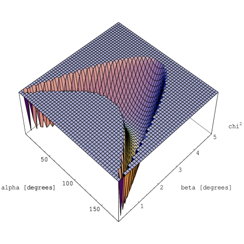
Figure 2: $\chi^{2}$ surface as a function of $\alpha$ and $\beta$ for pulsar B0301+19 Note that there is a long, deep, and virtually flat–bottomed chasm defined by the observed value of position angle sweep rate $d\psi/d\phi$, via Eq. 5.

At other times, the fit would never truly converge to an answer, but would instead indefinitely search for a minimum without finding one. The reason for the difficulty in fitting can be seen in a plot of the $\chi^{2}$ topography of a particular pulsar, P0301+19, in Fig 2, which is representative of most. (See also von Hoensbroech & Xilouris (1997a).) There is a deep chasm in $\chi^{2}$ space representing all $(\alpha,\beta)$ satisfying the observed position angle sweep via Eq. 5. Consequently the best–fitting solution $(\alpha_{best},\beta_{best})$ lies somewhere in the bottom of the chasm. Unfortunately, the floor of the entire valley lies at approximately the same “elevation,” resulting in a difficult–to–find minimum and hence a poorly defined best fit. Note then that it is even difficult to distinguish something as basic as inner and outer trajectories. This is a graphically–oriented description of the fact that $\alpha$ and $\beta$ are highly covariant as a result of the similarity of all RVM curves satisfying a particular value of Eq. 5, which is the limiting case of Eq. 1 over the small longitude range occupied by most pulsars’ emission.

Another problem is that many pulsars seem to have RVM–style polarization curves, but upon closer inspection, we discovered that the curve was of a slightly incorrect shape, and again, the fit would not converge. Due to difficulties like these, out of 70 pulsars for which we had average pulse position angle data, only ten could be fit reliably. The reliability of the fit was assessed by using other researchers’ results as initial parameter estimates for our algorithm. In each of the ten successful cases, all of our fits converged to the same final results, which often were not the same as the other published solutions. The results for our fits are listed in Table 3, along with values from other researchers for those same pulsars, which have all been converted to consistent definitions for $\alpha$ and $\beta$ via Table 1.

3.5 Calculating Errors on the Covariant Parameters

With the output from the fitting engine, we were able to calculate errors based on the full length of the region lying at $\Delta\chi^{2}_{\nu}=1$ above the minimum, which is imperative because $\alpha$ and $\beta$ are highly covariant (von Hoensbroech & Xilouris, 1997a; Press et al., 1992). The estimated uncertainties reported in Table 3 reflect the covariant relationship between parameters.

3.6 Results

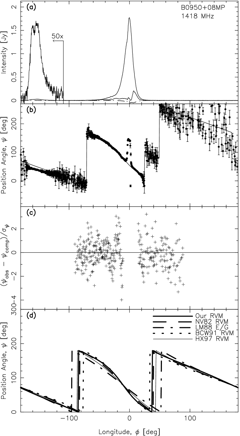
Figure 10: Pulsar B0950+08. Main pulse weighted, with the interpulse unweighted. For general explanation of this figure, see Fig. 3 and Fig. 6 captions. Note that a $90\arcdeg$ orthogonal mode switch is inserted in the longitude range $(25,170)\arcdeg$ and that longitudes between $(-180,-90)\arcdeg$, $(-10,15)\arcdeg$, and $(90,180)\arcdeg$ are unweighted in the fit shown in (b) and (c). We omit the same curves as in Fig. 8.

We describe here the results of our fits and compare them with other investigators’ efforts. The fits are shown in Figs. 3–17, and listed and compared with others’ in Table 3.

3.6.1 PSR B0301+19 (Fig. 3)

The two other RVM fits at frequencies similar to or below ours, NV82 and BCW91, obtain substantially different results from our fit. All three yield similar values of the ratio $\sin\alpha/\sin\beta$, as expected from Eq. 5. We find that the other two fits share similar $\beta$ and appear to have $\alpha$ related by $\pi-\alpha_{NV}\approx\alpha_{BCW}$ although we believe that we have reduced all results to common definitions. Note that this transformation would represent a switch from an inner to an outer line of sight trajectory. The disparities highlight the great difficulty in determining a unique $\alpha$ and $\beta$ from an RVM fit for these two highly covariant parameters. The HX97a,b fit is at a much higher frequency and not surprisingly has quite different parameters.

The high quality of our position angle data, representing $0.3d$ of integration at Arecibo Observatory, has enabled us to fit farther into the pulse profile wings than could the earlier RVM investigators. Apparently this extra longitude range permitted a more robust solution. It is quite interesting to note that our results are much closer to the two E/G investigations, which also are similar to each other.

3.6.2 PSR B0525+21 (Fig. 4)

The results in Table 3 appear rather scattered at first glance. However, We agree with BCQ to within a few $\sigma$, and the HX97a,b 1.41 GHz result would also agree if one took the complement of $\alpha_{HX}$ (switching from an inner to an outer line of sight trajectory). However, the two E/G results and the NV82, 0.43 GHz RVM fit place $\alpha$ far away, at or above $\sim 155\arcdeg.$ We favor our result, which is based on $1.9h$ of integration at Arecibo, again permitting a fit farther into the profile wings.

3.6.3 PSR B0656+14 (Fig. 5)

The low–level polarized emission between $(18-30)\arcdeg$ longitude provides part of the critical second half of the classic S–shaped RVM curve. It is this extra longitude coverage, resulting from a deep $1.8h$ integration, that enables the fit to converge to a unique value. Note that our fit moves $\phi_{0}$, the longitude of symmetry, to the end of the main pulse component, indicating that the main component and the trailing low–level emission constitute the opposite sides of a cone. There are no other RVM results on this pulsar. Our rather large error bars encompass the E/G results.

3.6.4 PSR B0823+26 (Figs. 6,7)

Both R93 and W99 have labelled the main component a core, based primarily on its polarization properties. (R93 called the whole profile $T$, while W99 labelled it $S_{t}$ based also on newer high–frequency observations.) The pulsar presents a main pulse plus a postcursor at $\phi\sim 40\arcdeg$ and a very weak interpulse near $\phi\sim 180\arcdeg$. An apparent orthogonal mode switch between $\phi=(-180$ and $-7)\arcdeg$ and $\phi=(+140$ and $+190)\arcdeg$ was included in the fit by adding $90\arcdeg$ to the position angle over that longitude range, while a region of competing orthogonal modes was unweighted in the $\phi=(-7$ to $-1)\arcdeg$ range. We present two sets of results – the preferred one to the full main / postcursor / interpulse component range, and another one to the first two components alone (see Table 4). The two results differ by several times their formal errors, a point to which we shall return below with pulsar B0950+08. Note also that our two results place $\alpha$ in (barely) opposite hemispheres. This seems rather unimportant until one realizes that the negative $\beta$ of both fits then implies an inner line of sight trajectory in one fit, but an outer trajectory in the other (see Section 1.1 and Table 2 for further discussion). However, the distinction between inner and outer is less important for equatorial trajectories such as these.

Our results comport with the other three RVM fits on this pulsar at similar frequencies: NV82, BCW91, and HX97a,b, although error bars on their results are generally quite large or not given. (A 0.43 GHz BCW91 fit with small error bars is also in quite good agreement with our 1.4 GHz results.) Both of the empirical/geometrical main–pulse results lie close to ours. LM88 also derive E/G results for the interpulse, as shown in Table 3. In addition, LM88 crudely fitted the RVM to a combination of 0.43 and 1.4 GHz position angle data for all three pulse components, with the result that $\alpha=100\arcdeg$, $\beta=-5.2\arcdeg$ (no uncertainties given). The fourth panel of Figs. 6 and 7, which shows the postion angle calculated from many workers’ results atop our data, demonstrates that our fit yields a better representation of our data than does any other published result. Our careful treatment of uncertainties and biases in the extensive low–level emission also favors our result.

It is clear from our fit that the interpulse represents emission from the opposite pole having $\alpha_{2}=81\fdg 1$, so $\beta_{2}=\zeta-\alpha_{2}=14\fdg 8$. This large impact parameter helps to explain why the interpulse is so much weaker than the main pulse. The postcursor is then emitted from the vicinity of the primary magnetic pole but at higher impact parameter than the main pulse.

3.6.5 PSR B0950+08 (Figs. 8, 9, 10)

In our preferred fit (Fig. 8), we use data from all longitudes, with the exception of the ranges $\phi=(-10$ to $+15)\arcdeg$. We also account for the orthogonal mode emission between $\phi=(25$ to $175)\arcdeg$. The resulting fit appears quite robust across virtually the whole fitted longitude range.

Our result is significantly at odds with all the others (including both RVM and E/G determinations), which are rougly consistent with each other. While our solution suggests a two–pole orthogonal rotator like B0823+26, the other fits (including an LM88 RVM fit to data stitched together from several sources yielding $(\alpha,\beta)=(170,4.6)\arcdeg$) place $\alpha\approx 170\arcdeg$ with both pulse and interpulse emission from a single pole. [Narayan & Vivekanand (1983b) and Gil (1983) elaborated a one–pole model for this pulsar.]

Our result indicates that the second pole has $\alpha_{2}=74\fdg 6$ and $\beta_{2}=52\fdg 9$. Hankins & Cordes (1981) showed that the main pulse–interpulse longitude separation remains constant between 40 and 4850 MHz, as expected of a two–pole emitter. However, the emission between the pulse and interpulse components is then particularly puzzling, as it is emitted even farther from the two magnetic poles than are the pulse and interpulse themselves.

Our two other solutions select data over narrower longitude ranges to test the consistency of our fits. (see Table 4 and Figs. 9 and 10). First, we unweight data in the vicinity of the main pulse, leaving what appears to be a fine fit across the interpulse and elsewhere (Fig. 9). The angles $\alpha$, $\beta$ and $\phi_{0}$ change significantly. The second additional fit unweights all data near the interpulse. Note that this “main pulse” fit looks quite reasonable throughout the fitted range (see Fig. 10), yet $\alpha$ and $\beta$ move from our preferred fit by several times the formal errors.

While both of these latter fits appear reasonable over their fitted ranges, they both fail elsewhere. Only the first, full longitude range fit, conforms well to observed position angles at all longitude ranges. We believe that our high–quality data, coupled with our careful treatment of measurement uncertainties in the fits, provide a more accurate result. For comparison, we superpose some of the other workers’ results, along with ours, onto our data in the bottom panel of each of Figs. 8, 9, and 10. Note that only our full fit (Fig. 8) matches well the overall slope of position angle with longitude over the longitude range $\sim-160$ to $-20\arcdeg$. (All results including ours have some trouble matching the left edge of the interpulse, presumably as a result of orthogonal mode competition.)

We are confident that our full range fit is the best one. However, our own three somewhat inconsistent solutions help to illustrate the pitfalls of RVM fitting. Since most other pulsars’ emission is detected over a much narrower longitude range, the resulting solutions could be expected to be no more representative of the actual situation at the pulsar than are the two restricted range fits discussed here. Presumably orthogonal mode mixing and/or other systematic effects cause these inconsistencies. Clearly the formal uncertainties generally underestimate the errors, as was also the case for pulsar B0823+26.

Similarly, the fact that other RVM investigators converged on a much different solution than we did (indicating a one–pole emitter rather than our two–pole orthogonal rotator) shows how sensitive the fitting process is to low–level emission which must be properly weighted.

3.6.6 PSR B1541+09 (Figs. 11, 12)

This pulsar has an unusually wide profile, which extends over $100\arcdeg$ in longitude. Unfortunately a large region, from $\sim-10$ to $\sim+35\arcdeg$ longitude, must be excluded in order to achieve convergence. Note that within the context of the RVM model, the only way to explain the reversal of sign of $d\psi/d\phi$ within the profile is to posit an outer line of sight trajectory, with the extremum in $\psi$ occuring at a longitude that is some distance from $\phi_{0}$ (Narayan & Vivekanand, 1982). Indeed our fit, after excluding the above noted range, conforms to these conditions. However, the full range of observed position angles cannot be fitted to any possible set of parameters in this scenario. More likely, emission in the excluded range represents the combination of two RVM orthogonal modes with relative amplitude varying across the excluded zone. Backer & Rankin (1980) show orthogonal mode competition is important at lower longitudes than these at 430 MHz; unfortunately there are apparently no 1.4 GHz orthogonal mode analyses.

There are no other published RVM fits, but the two E/G results (which are close to one another) are significantly at odds with ours. However, the position angles derived from both of their results bear no resemblance to the observed position angles, which leads us to doubt their efficacy, at least at our frequency of 1.4 GHz (see the bottom panels of Figs. 11 and 12).

Proceeding under the assumption that some or all of the data at longitudes below $\sim 35\arcdeg$ must be unweighted, we were able to obtain two convergent fits. In our preferred fit (see Fig. 11), the longitude range $(-8,+38)\arcdeg$ is unweighted, but lower longitudes fit quite well onto the RVM. In the second fit, all longitudes below $30\arcdeg$ are unweighted. The two fits yield rather different results for $\alpha,\beta,$ and $\phi_{0}$.

In our fits, the inflection point at $\sim 52$ or $\sim 62\arcdeg$ longitude represents the closest approach of the magnetic axis and the line of sight. It is interesting that the very strong circular polarization (among the strongest observed in any pulsar) occurs at longitudes similar to our excluded range, suggesting an unusual emission component much like a core except that it is not at the symmetry point, as expected. W99 reviewed all available multifrequency profile measurements and concluded that this pulsar is a classical triple ($T$), also identifying the highly circularly polarized component with the core. The current fit differs from their result in that it finds the symmetry center after the highly circularly polarized component, rather than in it. The leading component is then even farther from the symmetry center, rather than lying symmetrically opposite the trailing component.

3.6.7 PSR B1839+09 (Fig. 13)

Our result with $\alpha$ nearly $90\arcdeg$ and $\beta$ near $2\arcdeg$ agrees very well with the E/G analyses of R93 and LM88, in our fit encompassing $80\arcdeg$ of longitude. The only other RVM fit, from BCW91, did not achieve statistically significant results. Note that we unweighted the orthogonal mode competition starting at longitude $4\arcdeg$.

3.6.8 PSR B1915+13 (Fig. 14)

For this pulsar, we fit to all data within $60\arcdeg$ of longitude centered around the main pulse. The classical RVM sweep appears to fit the data well. Comparing our results to others, the BCW91 error bars on $\alpha$ and $\beta$ barely overlap with ours. As our fit is based on significantly more data, it is probably more reliable. The agreement with HX97a,b at 4.85 GHz is poorer, which is not surprising given the large frequency difference. The E/G results of R93a,b are the closest solutions to ours.

3.6.9 PSR B1916+14 (Fig. 15)

We fit the central $13\arcdeg$ of longitude. The only other RVM fit, from BCW91, has very large uncertainties which encompass our fit. Of the two E/G results, LM88 find $\alpha$ and $\beta$ near ours but the RVM curve derived from their parameters deviates significantly from our data, while R93a,b exhibits the opposite situation: her $\alpha$ and $\beta$ are far from ours but the RVM curve derived from her parameters matches our data well. The latter situation results from the strong covariance of the two parameters.

3.6.10 PSR B1929+10 (Figs. 16, 17)

For our preferred fit (Fig. 16), we fit all $360\arcdeg$ of longitude, except that we unweight the main pulse region from $-17\arcdeg$ to $+10\arcdeg$. The excluded region could not be fitted satisfactorily with the RVM curve, especially when trying to fit the interpulse and other off–pulse emission simultaneously with the main pulse. The single–pulse polarimetry of Rankin & Rathnasree (1997) [RR97] shows that indeed a competition between two orthogonal modes leads to position angle distortions in this region. Because the pulsar is so strong at these longitudes, our weighting scheme would otherwise cause this region to dominate the fit. We also placed a $90\arcdeg$ orthogonal mode offset from longitude $-60\arcdeg$ to $-15\arcdeg$, which is also evident in the single–pulse displays of RR97. Our second fit eliminates the main pulse entirely, (see Table 4 and Fig. 17)), and yields results roughly similar to the first.

Our $\alpha$ of approximately $35\arcdeg$ and $\beta\sim 26\arcdeg$ seems to be another shot at what seems a scatter of results for this pulsar. Other results not listed in Table 3 include the following RVM fits: LM88, using the 430 MHz data of Rankin & Benson (1981), found $(\alpha,\beta)=(15,7.5)\arcdeg$, Phillips (1990) [P90] measured $(\alpha,\beta)=(35\pm 4,21\pm 3)\arcdeg$ at 1665 MHz and $(\alpha,\beta)=(30\pm 2,20\pm 2)\arcdeg$ at 430 MHz, and RR97 found $(\alpha,\beta)=(31,20)\arcdeg$ at 430 MHz. Note that most of the RVM fits, including ours, yield roughly similar results, which indicate that the pulse and interpulse are emitted from nearly opposite sides of a wide, hollow cone near the $+\vec{\Omega}$ spin axis. While one can find the colatitude and impact parameter of the other magnetic pole as $\alpha_{2}=144\fdg 0$ and $\beta_{2}=-82\fdg 5$, these quantities are not important in a one–pole emission model. The significantly nonzero value of $\phi_{0}$ indicates that the brightest emission does not occur at closest approach of the line of sight and the magnetic axis. Aside from his choice of emission centered on the $-\vec{\Omega}$ spin axis, we are in agreement with the rough sketch of the emission geometry shown in P90.

R93, using E/G arguments, also found $(\alpha,\beta)=(18,11.6)\arcdeg$ if B1929+10 is interpreted as a $cT$–type pulsar, but suggested that it might be an orthogonal rotator if it is of the $T$ class. While the RR97 RVM fit discussed above also suggests a moderately tipped dipole, the authors argue that RVM fits lead to spurious results for this pulsar, and they favor an orthogonal rotator $(\alpha,\beta)\sim(90,0)\arcdeg$, dual pole emission model, again on the basis of E/G considerations. We still prefer our RVM results, as we believe it is unlikely that such a beautiful fit obtained over such a wide longitude range could be so seriously corrupted by systematic effects as to render it invalid.

4 Conclusions

We have fitted pulsar polarization data to the rotating vector model (RVM) in order to find geometrical parameters. We were careful to account properly for the bias in $L$ at low $S/N$ and for non–Gaussian statistics of position angle data, so that the low $S/N$ data could be appropriately weighted in the fits. This enabled us to correctly include low–level emission arising from weak pulse components as well as the wings of main components in the fits. We are not aware of any other RVM fits that include such considerations.

We succeeded in finding convergent RVM fits on ten of the pulsars observed by Weisberg et al. (1999). In all such cases, we always converged to our same solution regardless of our choice of initial parameters gleaned from previously published results. Yet we were surprised that our fitting procedure converged for relatively few of the many pulsars for which we had high–quality data. Presumably this was due to competition between orthogonal emission modes or other systematic effects. Because of the high covariance between the two important fitted parameters $\alpha$ and $\beta$, even slight deviations of position angle data from the nominal RVM model could prevent convergence to a unique solution. Wide longitude ranges of emission were generally required in order to achieve unique, convergent fits. As a result, pulsars with interpulses and/or other off pulse emission are favored targets for RVM studies. Nevertheless, we show that in two such cases (pulsars B0823+26 and B0950+08), our fits to different longitude ranges yield results differing by several times their formal errors. Consequently it is clear that systematic effects are present at a significant level.

We created transformation equations to convert other published RVM and empirical–geometrical (E/G) results to a common definition, in order to compare them with our results and to facilitate future comparisons. For some pulsars, all workers’ results are similar while for others there is a wide range of solutions. No clear pattern emerges from these comparisons.

We are currently in the process of separating orthogonal modes in single pulse polarization data (Weisberg & Everett, 2001), in order to to determine if RVM fits to separated emission modes yield results different than the average pulse results presented here.

Figure 1: In the rotating vector model (RVM, see Eq. 1), the magnetic pole colatitude $\alpha$, line of sight colatitude $\zeta$, and line of sight impact parameter $\beta$ are defined in terms of the positive angular velocity vector $+\vec{\Omega}$ and the observable magnetic pole $\mu$. These quantities are shown here in the plane containing $\vec{\Omega}$ and $\mu$. Note that these definitions are the same for all possible $\alpha$; i.e., for $(0\leq\alpha\leq\pi)$ radians.

Figure 3: Pulsar B0301+19: (a): Total ($I$), linearly polarized ($L$), and circularly polarized ($V$, dashed–dotted), flux densities; (b): Observed and fitted position angle of linear polarization $\psi$ with error bars representing measurement uncertainties; and (c): Position angle residuals, normalized by $\sigma_{\psi}$. The fit was allowed to extend over the full displayed longitude range.

Figure 4: Pulsar B0525+21: See Fig. 3 caption for details.

Figure 5: Pulsar B0656+14 See Fig. 3 caption for details.

Figure 6: Pulsar B0823+26. Our preferred full longitude fit. For an explanation of (a) – (c), see Fig. 3 caption. Note that a $90\arcdeg$ orthogonal mode switch is inserted in the longitude range $(-180,-7)\arcdeg$ and $(+140,+180)\arcdeg$, and that longitudes between $(-7,-1)\arcdeg$ are unweighted in the fit. Panel (d) shows the RVM curves from our and other investigators’ work. Orthogonal mode jumps included in our fit and shown in (b) and implicitly in residuals (c) are not included in (d), in order to simplify comparison with other authors’ work. Also, since other investigators generally did not provide their fitted position angle and longitude offsets $\psi_{0}$ and $\phi_{0}$, we use our values of these two parameters in calculations of their RVM curves. At the resolution of panel (d), the NV82 RVM is indistiguishable from ours, so we do not plot it.

Figure 7: Pulsar B0823+26. Main pulse through postcursor fit. For general explanation of this figure, see Fig. 3 and Fig. 6 captions. Note that a $90\arcdeg$ orthogonal mode switch is inserted in the longitude range $(-20,-7)\arcdeg$ and that longitudes between $(-7,-1)\arcdeg$ are unweighted in the fits shown in (b) and (c). At the resolution of panel (d), both the BCW91 RVM and the NV82 RVM are indistiguishable from ours, so we do not plot them. Also, the HX97 RVM curve overlays the LM88 E/G curve, so we do not plot the HX97 RVM fit.

Figure 8: Pulsar B0950+08. Our preferred full longitude fit. For general explanation of this figure, see Fig. 3 and Fig. 6 captions. Note that a $90\arcdeg$ orthogonal mode switch is inserted in the longitude range $(25,175)\arcdeg$ and that longitudes between $(-10,+15)\arcdeg$ are unweighted in the fits shown in (b) and (c). At the resolution of panel (d), the R93 E/G curve is indistiguishable from the LM88 E/G curve, so we do not plot the R93 E/G curve.

Figure 9: Pulsar B0950+08. The interpulse is weighted in this fit, with the main pulse ($\phi=(-90,90)\arcdeg$) unweighted. For general explanation of this figure, see Fig. 3 and Fig. 6 captions. Note that a $90\arcdeg$ orthogonal mode switch is inserted in the longitude range $(25,170)\arcdeg$ and that longitudes between $(-90,90)\arcdeg$ are unweighted in the fits shown in (b) and (c). We omit the same curves as in Fig. 8.

Figure 11: Pulsar B1541+09. Our preferred wide longitude fit. For general explanation of this figure, see Fig. 3 and Fig. 6 captions. Longitudes between $(-8,+38)\arcdeg$ are unweighted in the fit shown in (b) and (c). The R93 curve in panel (d), which appears to have the wrong slope, corresponds to $(\alpha,\beta)=(175,0)$, which represents a line of sight traverse right across the magnetic pole. Even a slight nonzero $\beta$ would add a region of inverted slope near $\phi=\phi_{0}$, which would better match our data.

Figure 12: Pulsar B1541+09. Narrower longitude fit. For general explanation of this figure, see Fig. 3 and Fig. 6 captions. All longitudes below $30\arcdeg$ are unweighted in in this alternative fit shown in (b) and (c). See Fig. 11 for a discussion of the R93 curve in (d).

Figure 13: Pulsar B1839+09. See Fig. 3 caption for details. Longitudes between $(+4,+10)\arcdeg$ are unweighted in the fit.

Figure 14: Pulsar B1915+13. See Fig. 3 caption for details.

Figure 15: Pulsar B1916+14. For a general explanation of this figure, see Fig. 3 and Fig. 6 captions. At the resolution of panel (d), the R93 E/G curves is indistiguishable from the BCW91 curve, so we do not plot the R93 E/G curve.

Figure 16: Pulsar B1929+10. Our preferred full longitude fit. For general explanation of this figure, see Fig. 3 and Fig. 6 captions. Note that a $90\arcdeg$ orthogonal mode switch is inserted in the longitude range $(-60,-15)\arcdeg$ and that longitudes between $(-17,+10)\arcdeg$ are unweighted in the fits shown in (b) and (c). Our preferred RVM curve and most other published RVM fits provide the best match to the data. At the resolution of panel (d), the NV82 RVM, RR97 RVM (their fit), and BCW91 RVM curves are indistiguishable from our curve, so we do not plot them. Also, the LM88 RVM (their fit) curve is indistinguishable from the LM88 E/G (their empirical calculation) curve, so we do not plot the LM88 RVM curve.

Figure 17: Pulsar B1929+10. Entire main pulse region unweighted. For general explanation of this figure, see Fig. 3 and Fig. 6 captions. Note that a $90\arcdeg$ orthogonal mode switch is inserted in the longitude range $(-60,-15)\arcdeg$ and that longitudes between $(-17,+10)\arcdeg$ are unweighted in the fits shown in (b) and (c). Our RVM curve and most other published RVM fits provide the best match to the data. We omit the same curves as in Fig. 16.

Table 1: Dictionary and Conversion Table from Earlier Work for Geometrical Beam Parameters. (See Eqs. 1 and 2 and ensuing discussion.)

Investigators	$\psi$	Colatitude of Observable Magnetic Pole, $\alpha$		Impact Parameter of Line of Sight
and	Convention	w.r.t. ($+\vec{\Omega}$) Spin Axis		w.r.t. Observable Magnetic Pole
Method	Problem?	Confined	Relation to	Symbol in	Relation to
		to First	our $\alpha$	Original	our $\beta$
		Quadrant?	($\alpha_{original}\rightarrow$ our $\alpha$)	Paper	($Symbol_{original}\rightarrow$ our $\beta$)
Current Work	no	no	$\alpha\rightarrow\alpha$	$\beta$	$\beta\rightarrow\beta$
(RVM)
NV82	no	yes	If $(d\psi/d\phi$ and $\beta_{NV})$	$\beta_{NV}$	If $d\psi/d\phi>0$, then
(RVM)			both have same sign, then		$-|\beta_{NV}|\rightarrow\beta.$
			$\pi-\alpha_{NV}\rightarrow\alpha.$		If $d\psi/d\phi<0$, then
			Otherwise, $\alpha_{NV}\rightarrow\alpha.$		$|\beta_{NV}|\rightarrow\beta.$
LM88	n/a	yes	As the sign of $\beta_{LM}$ was not	$\beta_{LM}$	If $d\psi/d\phi>0$, then
(E/G)			published, either $\alpha_{LM}\rightarrow\alpha$	(magnitude only	$-|\beta_{LM}|\rightarrow\beta.$
			or $\pi-\alpha_{LM}\rightarrow\alpha$ are possible.	was published)	If $d\psi/d\phi<0$, then
			We selected one based on con-		$|\beta_{LM}|\rightarrow\beta.$
			sistency with our fits.
BCW91	yes	no	$\pi-\alpha_{BCW}\rightarrow\alpha.$	$\sigma_{BCW}$	$\sigma_{BCW}\rightarrow-\beta$
(RVM)
R90,93a,b	n/a	yes	If $(d\psi/d\phi$ and $\beta_{R})$	$\beta_{R}$	If $d\psi/d\phi>0$, then
(E/G)			both have same sign, then		$-|\beta_{R}|\rightarrow\beta.$
			$\pi-\alpha_{R}\rightarrow\alpha.$		If $d\psi/d\phi<0$, then
			Otherwise, $\alpha_{R}\rightarrow\alpha.$		$|\beta_{R}|\rightarrow\beta.$
HX97a,b	yes	no	$\pi-|\alpha_{HX}|\rightarrow\alpha.$	$\sigma_{HX}$	If $\alpha_{HX}>0$, then
(RVM)					$\sigma_{HX}\rightarrow-\beta.$
					Otherwise, $\sigma_{HX}\rightarrow\beta.^{a}$

Table 2: Inner and Outer Line of Sight Trajectories

Sign of	Sign of	Sign of Impact Param.	Colatitude of	Line of Sight Trajectory
Slopea	Slopeb	of Line of Sight w.r.t.	Observable Mag-	w.r.t.
$\frac{d\psi}{d\phi}|_{max}$	$\frac{d\psi^{\prime}}{d\phi}|_{max}$	Obs. Mag. Pole, $\beta$	netic Pole, $\alpha$	Observable Magnetic Pole
			$<\pi/2$	Outer (Equatorward)c
Negative	Positive	Positive
			$>\pi/2$	Inner (Nearest $[-\vec{\Omega}]$ Spin Poleward)
			$<\pi/2$	Inner (Nearest $[+\vec{\Omega}]$ Spin Poleward)
Positive	Negative	Negative
			$>\pi/2$	Outer (Equatorward)c

Table 3: Geometrical angles $\alpha$ and $\beta$ from our work and other investigators.’ All angles have been converted to a common definition using Table 1.

Pulsar	R93a,b	Our adopted results				NV82		LM88		BCW91			R93a,b		HX97a,b
	Class.	(1.42 GHz)				(0.43 GHz)		(0.4 GHz)					1 GHz
		(RVM)				(RVM)		(E/G)		(RVM)			(E/G)		(RVM)
		$\alpha$	$\beta$	$\phi_{0}$	$\chi_{\nu}^{2}$	$\alpha$	$\beta$	$\alpha$	$\beta$	$\nu$ (GHz)	$\alpha$	$\beta$	$\alpha$	$\beta$	$\nu$ (GHz)	$\alpha$	$\beta$
0301+19	$D$	162.4	0.96	-3.71	15.6	110	3	148.1	1.8	1.42	69	2.9	150	1.7	4.85	85.7	13.9
		$\pm 11.8$	$\pm 0.63$	$\pm 0.006$		$\pm 11$					$\pm 16$	$\pm 0.3$				$\pm 15.0$	$\pm 15.0$
										0.43	61	2.8
											$\pm 30$	$\pm 0.4$
0525+21	$D$	116.8	-1.50	-5.84	7.9	$\geq 160$	-0.6	156.8	-0.7	1.42	134	-1.2	159	-0.6	1.41	44.2	-1.3
		$\pm 4.6$	$\pm 0.08$	$\pm 0.02$							$\pm 10$	$\pm 0.2$				$\pm 60$	$\pm 0.2$
										0.43	140	-1.0			1.71	113.7	-2.0
											$\pm 9$	$\pm 0.2$				$\pm 80$	$\pm 1.0$
															4.85	162.2	-0.6
																$\pm 70$	$\pm 2.0$
0656+14	$T^{a}$	29	8.9	14.9	2.6			8.2	8.2				30
		$\pm 23$	$\pm 6.1$	$\pm 0.7$
0823+26	$S_{t}$	98.9	-3.03	1.33	8.6	98	-4	76.9	-1.1	1.42	89	-3	84	$-1.9^{b}$	$1.41^{c}$	90.2	-1.0
		$\pm 0.7$	$\pm 0.01$	$\pm 0.01$							$\pm 600$	$\pm 1$				$\pm 25$	$\pm 0.2$
(Main /										0.43	101	-3.2			$1.71^{c}$	97.7	-1.7
											$\pm 1$	$\pm 0.3$				$\pm 80$	$\pm 1.5$
Postcursor)															$4.85^{c}$	82.5	12.1
																$\pm$ 15	$\pm$ 15
Interpulse								$\pm 26.1$	5.6
0950+08	$S_{d}$	105.4	22.1	-11.9	2.2	170	5	174.1	4.2	1.42	174	2.5	168	8.5	1.41	179.3	0.4
		$\pm 0.5$	$\pm 0.1$	$\pm 0.2$							$\pm 30$	$\pm 15$				$\pm 15$	$\pm 15$
(Full)										0.43	174	2.5			4.85	153.1	4.1
											$\pm 90$	$\pm 40$				$\pm 90$	$\pm 5$
1541+09	$T$	131.0	-20.23	62.5	1.5			174.2	-0.8				175	0.0
		$\pm 5.67$	$\pm 2.26$	$\pm 0.37$
1839+09	$T$	86.1	2.3	0.34	10.3			90	2.9	1.42	146	1	97	$1.4^{b}$
		$\pm 11.4$	$\pm 0.04$	$\pm 0.02$							$\pm 400$	$\pm 8$
1915+13	$S_{t}$	73	5.4	6.8	4.2					1.42	86	5.4	68	6.6	4.85	89.3	9.3
		$\pm 19.4$	$\pm 0.5$	$\pm 0.1$							$\pm 24$	$\pm 0.2$				$\pm 12.5$	$\pm 15$
1916+14	$T(?)$	118.0	$-$1.0	0.38	8.9			124.5	-2.1	1.42	167	-0.3	101	-1.3
		$\pm 33.4$	$\pm 0.33$	$\pm 0.01$							$\pm 100$	$\pm 0.2$
$1929+10^{d}$	$T(?)/$	35.97	25.55	-19.62	2.45	35	23	6	4	1.42	27	16	$90^{f}$	41.8
		$\pm 0.95$	$\pm 0.87$	$\pm 0.2$							$\pm 4$	$\pm 3$
	$cT$									$1.42^{e}$	150	-3	$18^{f}$	11.6
											$\pm 10$	$\pm 2$
										0.43	25	16
											$\pm 2$	$\pm 2$
Interpulse													88

Note. — (a) In one case, (PSR B0950+08 at 1.41 GHz), the resulting $\zeta$ would then be greater than $\pi.$ Consequently, $2|\alpha_{HX}|-\sigma_{HX}\rightarrow\beta$ must instead be used.

Note. — (a) The quantity $\frac{d\psi}{d\phi}|_{max}$ is the position angle sweep rate in the observers’ convention (increasing counterclockwise on the sky), while (b) $\frac{d\psi^{\prime}}{d\phi}|_{max}$ is the sweep rate in the (opposite) RVM convention. (c) “Equatorward” indicates that the line of sight is opposite the spin pole lying nearest to the observable magnetic pole.

Note. — (a) W99 suggest $S_{t}$; (b) Here we choose opposite sign as R93a,b, as required by Eq. (5); (c) Main pulse only; (d) See text for additional RVM fits by LM88,P90, and RR97; (e) Alternate BCW91 fit; (f) First Rankin fit is under assumption of $T$ classification; second is for $cT$.

Table 4: Multiple convergent fits to pulsars with multiple components.

Pulsar	Components fitted	Longitude	Our results
		limitsa	$\alpha$	$\beta$	$\phi_{0}$	$\chi_{\nu}^{2}$
0823+26	full	$\pm$180	98.9	-3.03	1.33	8.6
			$\pm$ 0.7	$\pm$ 0.01	$\pm$ 0.01
	main / postcursor	$-20$ to $45$	85.8	-3.08	1.21	8.6
			$\pm$ 3.2	$\pm$ 0.01	$\pm$ 0.02
0950+08	full	$\pm 180$	105.4	22.1	-11.9	2.2
			$\pm$ 0.5	$\pm$ 0.1	$\pm$ 0.2
	main pulse	$-90$ to $+90$	126.2	19.6	-10.8	1.3
			$\pm$ 4.3	$\pm$1.0	$\pm$ 0.3
	interpulse	$+90$ to $-90$	109.6	13.3	-37.6	2.3
			$\pm$ 1.4	$\pm$ 0.9	$\pm$5.3
1929+10	full	$\pm 180$	35.97	25.55	-19.62	2.45
			$\pm$ 0.95	$\pm$ 0.87	$\pm$ 0.2
	interpulse	$-180$ to $-40$	34.3	28.8	-20.2	2.5
		$35$ to $180$	$\pm$ 0.86	$\pm$0.23	$\pm$ 1.2

Note. — (a) See text and figure captions to find ranges of unweighted longitudes within these limits.

References

- Arzoumanian et al. (1996) Arzoumanian, Z., Phillips, J.A., Taylor, J.H., Wolsczaan, A. 1996, ApJ, 470, 1111
- Backer & Rankin (1980) Backer, D.C., Rankin, J.M. 1980, ApJS, 42, 143
- Biggs (1990) Biggs, J.D. 1990, MNRAS, 245, 514
- Biggs (1992) Biggs, J.D. 1992, ApJ, 394, 574
- Bjornsson (1998) Bjornsson, C.-I. 1998, A&A, 338, 971
- Blaskiewicz et. al. (1991) Blaskiewicz, M., Cordes, J.M., Wasserman, I. 1991, ApJ, 370, 643 (BCW91)
- Candy & Blair (1986) Candy, B.N., Blair, D.G. 1986, ApJ, 307, 535
- Damour & Taylor (1992) Damour, T., Taylor, J.H. 1992, Phys. Rev. D, 45, 1840
- Gil et al. (1991) Gil, J.A., Snakowski, J.K., Stinebring, D.R. 1991, A&A, 242, 119
- Gil (1983) Gil, J. 1983, A&A, 127, 267
- Hankins & Cordes (1981) Hankins, T.H., Cordes, J.M. 1981, ApJ, 249, 241
- von Hoensbroech & Xilouris (1997a) von Hoensbroech, A., Xilouris, K.M. 1997a, A&A, 324, 981 (HX97a)
- von Hoensbroech & Xilouris (1997a,b) von Hoensbroech, A., Xilouris, K.M. 1997b, A&AS, 126, 121 (HX97b)
- Jones (1980) Jones, P.B. 1980, ApJ, 236, 661
- Lyne & Manchester (1988) Lyne, A.G., Manchester, R.N. 1988, MNRAS, 234, 477 (LM88)
- Manchester, Han, & Qiao (1998) Manchester, R.N., Han, J.L., Qiao, G.J. 1998, MNRAS, 295, 280
- McKinnon (1993) McKinnon, M.M. 1993, ApJ, 413, 317
- Miller & Hamilton (1993) Miller, M.C., Hamilton, R.J. 1993, ApJ, 411, 298
- Naghizadeh-Khouei & Clarke (1993) Naghizadeh-Khouei, J., Clarke, D. 1993, A&A, 274, 968