Precessing warped accretion discs in X-ray binaries

Abstract

We study the radiation-driven warping of accretion discs in the context of X-ray binaries. The latest evolutionary equations are adopted, which extend the classical alpha theory to time-dependent thin discs with non-linear warps. We also develop accurate, analytical expressions for the tidal torque and the radiation torque, including self-shadowing.

We investigate the possible non-linear dynamics of the system within the framework of bifurcation theory. First, we re-examine the stability of an initially flat disc to the Pringle instability. Then we compute directly the branches of non-linear solutions representing steadily precessing discs. Finally, we determine the stability of the non-linear solutions. Each problem involves only ordinary differential equations, allowing a rapid, accurate and well resolved solution.

We find that radiation-driven warping is probably not a common occurrence in low-mass X-ray binaries. We also find that stable, steadily precessing discs exist for a narrow range of parameters close to the stability limit. This could explain why so few systems show clear, repeatable ‘super-orbital’ variations. The best examples of such systems, Her X-1, SS 433 and LMC X-4, all lie close to the stability limit for a reasonable choice of parameters. Systems far from the stability limit, including Cyg X-2, Cen X-3 and SMC X-1, probably experience quasi-periodic or chaotic variability as first noticed by Wijers & Pringle. We show that radiation-driven warping provides a coherent and persuasive framework but that it does not provide a generic explanation for the long-term variabilities in all X-ray binaries.

1 Introduction

A growing number of X-ray binaries are known to exhibit more or less periodic variability on time-scales much longer than their orbital periods (see Priedhorsky & Holt 1987; Smale & Lochner 1992; White, Nagase & Parmar 1995; Corbet & Peele 1997). The clearest examples of such ‘super-orbital’ periods can be found in Her X-1, SS 433 and LMC X-4. They have been known for a long time and are well documented. Different explanations have been proposed for the long periods of these systems but there seems to be a converging opinion, from both the observational and theoretical viewpoints, that these periods represent the precession of a tilted accretion disc (Katz 1973; Petterson 1975; Schwarzenberg-Czerny 1992; Wijers & Pringle 1999 and references therein). As well as periodically obscuring the X-ray source, a tilted disc casts an asymmetric shadow on the irradiated companion star which well reproduces the optical light-curves (e.g. Gerend & Boynton 1976; Leibowitz 1984; Heemskerk & van Paradijs 1989; Still et al. 1997).

It has long been recognized that the precession of a tilted disc could be caused by the tidal force of the companion star (Katz 1973). Consider the disc to be composed of a sequence of concentric circular rings, tilted with respect to the binary orbital plane. The rings behave gyroscopically owing to their rapid rotation. If they did not interact with each other, the tidal torque would cause each ring to precess retrogradely, about an axis perpendicular to the binary plane, at a rate that depends on the radius of the ring, resulting in a rapid twisting of the disc. However, a fluid disc tends to resist this by establishing an internal torque between neighbouring rings. This can be arranged so that the net torque on each ring is such as to produce a single, uniform precession rate, allowing the disc to precess coherently. However, the internal torque can only be established if the disc becomes warped. This is accompanied by dissipation of energy and the disc settles into the binary plane (Lubow & Ogilvie 2000; Bate et al. 2000).

A mechanism is therefore required to excite the tilt continuously. Radiation-driven warping has been identified as a plausible way to do this. If the outer part of the disc is warped, it intercepts radiation from the central point source. If this radiation is absorbed and re-emitted parallel to the local normal to the disc surface, the disc experiences a torque from the radiation pressure (Petterson 1977; Pringle 1996). The albedo of the disc is probably irrelevant since scattered photons leaving the disc will also have a distribution of momenta peaked around the local normal (see Appendix A4). A small tilt grows exponentially if it is twisted such that the line of nodes forms a leading spiral, and if the luminosity is sufficient to overcome dissipative processes that tend to flatten the disc (Pringle 1996).

Such a mechanism would apply very well to X-ray binaries where the optical emission of the accretion disc is dominated by X-ray reprocessing (van Paradijs & McClintock 1994). This does not preclude other driving mechanisms for warps, in particular wind torques (Schandl & Meyer 1994), but radiation-driven warping does have the advantage of relying on well-defined physics.

The first question to be addressed is whether an initially flat disc is unstable to radiation-driven warping. Previous studies (Pringle 1996; Maloney, Begelman & Pringle 1996; Maloney & Begelman 1997; Maloney, Begelman & Nowak 1998) concluded that discs in X-ray binaries are indeed likely to be unstable. Although instructive, these studies neglected self-shadowing of the disc and were not satisfying in their treatment of the boundary conditions, which can be crucial to this problem. Furthermore, there was some uncertainty as to what equations to use. Recent progress (Ogilvie 1999, 2000) has led to a practical set of equations describing non-linear warps in thin discs. Although only one-dimensional, the equations are derived directly from the basic fluid-dynamical equations in three dimensions, within the context of the alpha theory.

The second question concerns the non-linear development of the instability. In particular, does it lead to steadily precessing discs as suggested by observations of some systems? Recently, Wijers & Pringle (1999) investigated numerically the non-linear evolution of the instability and found a complex variety of behaviour. Their study was based on a direct integration of the earlier evolutionary equations of Pringle (1992). The calculations were restricted to low resolution owing mainly to the laborious treatment of self-shadowing.

In this paper, we present a complementary study to that of Wijers & Pringle (1999). In Section 2 we present our formulation of the dynamical problem, based on the new evolutionary equations of Ogilvie (2000). We also derive accurate, analytical expressions for the tidal torque and the radiation torque, including self-shadowing (see the Appendices). In Section 3 we re-examine the stability of an initially flat disc to radiation-driven warping. We then search directly for non-linear solutions representing steadily precessing discs and determine their stability (Section 4). All this can be achieved with high precision and resolution because it involves solving only ordinary differential equations (ODEs). These solutions would be directly applicable to systems such as Her X-1. Finally, in Section 5 we compare our results with observations. For the most part, we investigate generic properties in this paper, and leave the detailed modelling of individual systems to future work.

2 Dynamics of warped discs

2.1 Background

In general, the dynamics of a warped accretion disc in an X-ray binary is an extremely difficult problem of radiation magnetohydrodynamics in three dimensions. Furthermore, the evolution must be followed for many times longer than the characteristic orbital time-scale of the disc if one is to account for the observed behaviour. These considerations mean that an ab initio direct numerical treatment of the problem is completely unfeasible at present.

Considerable progress has been made in recent years towards developing a reduced description of warped accretion discs that is only one-dimensional and follows the evolution on the long, viscous time-scale. This approach was introduced by Papaloizou & Pringle (1983) and developed by Pringle (1992). It is based on writing down plausible conservation equations in one dimension for a disc composed of a continuum of thin circular rings that are in centrifugal balance but have varying inclinations. The rings interact by means of viscous torques.

Although this approach is intentionally simplistic in origin (Papaloizou & Pringle 1983), it has been shown that the same form of equations, with minor modifications, can be derived formally from the Navier-Stokes equation in three dimensions (Ogilvie 1999). This derivation also provides the non-trivial relation between the effective viscosity coefficients appearing in the reduced equations and the small-scale effective viscosity that acts on motions with a length-scale comparable to the disc thickness. The resulting theory can then be seen as a non-linear extension of the existing linear theory of bending waves in viscous Keplerian discs (Papaloizou & Pringle 1983).

To make this derivation possible, of course, certain assumptions must be made. The first is that the disc is thin, which is expected to be satisfied under a wide range of conditions. Indeed, the resulting theory is formally an asymptotic theory for thin discs. The second is that the agent responsible for angular momentum transport in accretion discs can be treated as an isotropic effective viscosity. Although it is now widely believed that this agent is magnetohydrodynamic turbulence resulting from the magnetorotational instability (Balbus & Hawley 1998), our understanding of how the turbulence responds to imposed motions other than a Keplerian shear flow is extremely limited (Abramowicz, Brandenburg & Lasota 1996). A first attempt to measure this response for motions of the type induced in a warped disc (Torkelsson et al. 2000) suggests that the assumption of an isotropic effective viscosity may be reasonable as a first approximation, and, in any case, no better model has been proposed. The third assumption is that the resonant bending-wave propagation found in inviscid, Keplerian discs may be neglected. This condition is satisfied if the viscosity parameter exceeds the angular semi-thickness of the disc ($\alpha\ga H/r$). Further assumptions are of a more technical nature, but include the assumption that the fluid is polytropic.

In a recent paper (Ogilvie 2000) this method was extended to include non-trivial thermodynamics. Instead of assuming the fluid to be polytropic, one now accounts fully for viscous dissipation and radiative energy transport within the Rosseland approximation. The fluid is treated as an ideal gas, and a power-law opacity function, such as Thomson or Kramers opacity, is assumed. The resulting theory forms a closed system and may be considered as the logical extension of the alpha-disc theory (Shakura & Sunyaev 1973) to time-dependent, warped accretion discs. In the absence of a warp, it reduces exactly to the usual alpha theory, except that the vertical structure of the disc is computed accurately by solving the differential equations, rather than by the usual algebraic approximations.

2.2 Basic equations

We consider a binary system with a compact star (or black hole) of mass $M_{1}$, about which the disc orbits, and a companion star of mass $M_{2}$, in a circular orbit of radius $r_{\rm b}$ and angular frequency

$$\Omega_{\rm b}=\left[{{G(M_{1}+M_{2})}\over{r_{\rm b}^{3}}}\right]^{1/2}.$$ (1)

We adopt Cartesian coordinates $(x,y,z)$ in a non-rotating frame of reference centred on the compact star, such that the orbit of the companion lies in the $xy$-plane and has a positive sense.

The dynamical system is described by partial differential equations in coordinates $(r,t)$, where $r$ is the distance from the central object and $t$ is the time. At radius $r$, the disc rotates in centrifugal balance, with orbital angular velocity $\Omega(r)$ and specific angular momentum $h(r)=r^{2}\Omega$. The state of the disc is characterized by a surface density $\Sigma(r,t)$ and a tilt vector $\mbox{\boldmath$l$}(r,t)$, which is a unit vector parallel to the local orbital angular momentum of the disc. The orbital angular momentum density is then $\mbox{\boldmath$L$}(r,t)=\Sigma h\,\mbox{\boldmath$l$}$. Throughout this paper we take the angular velocity to be Keplerian, i.e. $\Omega=(GM_{1}/r^{3})^{1/2}$.

The general forms of the conservation equations for mass and angular momentum are

$${{\partial\Sigma}\over{\partial t}}+{{1}\over{r}}{{\partial}\over{\partial r}}(rv\Sigma)=S$$ (2)

and

$${{\partial\mbox{\boldmath$L$}}\over{\partial t}}+{{1}\over{r}}{{\partial}\over{\partial r}}(rv\mbox{\boldmath$L$})={{1}\over{r}}{{\partial\mbox{\boldmath$G$}}\over{\partial r}}+\mbox{\boldmath$T$},$$ (3)

respectively. Here $v(r,t)$ is the mean radial velocity and $2\pi\mbox{\boldmath$G$}(r,t)$ is the internal torque in the disc. The terms $S(r,t)$ and $\mbox{\boldmath$T$}(r,t)$ represent the sources (per unit area) of mass and angular momentum, respectively. If necessary, these terms should be considered as the mean sources averaged over the orbital time-scale.

The total external torque consists of three parts,

$$\mbox{\boldmath$T$}=\mbox{\boldmath$T$}_{\rm add}+\mbox{\boldmath$T$}_{\rm rad}+\mbox{\boldmath$T$}_{\rm tide}.$$ (4)

The first represents the angular momentum added to the disc along with the accretion stream. The radiation torque $\mbox{\boldmath$T$}_{\rm rad}$, including the effects of self-shadowing, is evaluated in Appendix A, where we find (cf. equation 71)

$$\mbox{\boldmath$T$}_{\rm rad}=-{{L_{\star}}\over{12\pi rc}}\,\mbox{\boldmath$l$}\times\mbox{\boldmath$a$}.$$ (5)

Here $L_{\star}$ is the luminosity of the central source (assumed isotropic), $c$ the speed of light and $a$ a dimensionless vector depending on the shape of the disc. The tidal torque $\mbox{\boldmath$T$}_{\rm tide}$, averaged over the binary orbit, is evaluated in Appendix B, where we find (cf. equation 94)

$$\mbox{\boldmath$T$}_{\rm tide}=-{{3GM_{2}\Sigma r^{2}}\over{4r_{\rm b}^{3}}}(\mbox{\boldmath$e$}_{z}\cdot\mbox{\boldmath$l$})(\mbox{\boldmath$e$}_{z}\times\mbox{\boldmath$l$})\left(1+\cdots\right).$$ (6)

The final factor (not shown explicitly here) represents an advance over previous work; to omit it typically results in an error of $15\%$ at $r/r_{\rm b}=0.3$. Any other potential torques, such as self-gravitational, magnetic or gravitomagnetic torques, are neglected. Note that the acceleration of the origin of the coordinate system does not contribute a torque (Wijers & Pringle 1999).

2.2.1 Internal torque

Detailed analysis of the internal hydrodynamics of a warped disc (Ogilvie 1999, 2000) results in an expression for the internal torque of the form

$$\mbox{\boldmath$G$}={\cal I}r^{2}\Omega^{2}\left(Q_{1}\,\mbox{\boldmath$l$}+Q_{2}r{{\partial\mbox{\boldmath$l$}}\over{\partial r}}+Q_{3}r\,\mbox{\boldmath$l$}\times{{\partial\mbox{\boldmath$l$}}\over{\partial r}}\right),$$ (7)

where

$${\cal I}=\Big{\langle}\int\rho z^{2}\,{\rm d}z\Big{\rangle}$$ (8)

is the second vertical moment of the density, and $Q_{1}$, $Q_{2}$ and $Q_{3}$ are dimensionless coefficients. (In this definition only, $z$ denotes the distance from the mid-plane of the warped disc, and the angle brackets denote azimuthal averaging.) The generalized alpha theory (Ogilvie 2000) provides a relation between ${\cal I}$ and $\Sigma$ of the form

$${\cal I}=Q_{5}C_{\cal I}\alpha^{1/7}\Sigma^{10/7}\Omega^{-12/7},$$ (9)

where $Q_{5}$ is a further dimensionless coefficient, equal to unity for a flat disc, $C_{\cal I}$ is a constant, and $\alpha$ is the dimensionless viscosity parameter. It is assumed here that the disc is Keplerian and gas-pressure-dominated, and that the opacity law is of the Kramers form $\kappa\propto\rho T^{-7/2}$. The value of the constant $C_{\cal I}$ is approximately $4.4\times 10^{12}$ in CGS units (${\rm cm}^{20/7}{\rm g}^{-3/7}{\rm s}^{-12/7}$) (Ogilvie 2000). Although in the inner parts of the disc Thomson opacity may in fact dominate, and radiation pressure may be important, it will be seen that these inner parts play only a passive role in the dynamics, and equation (9) is sufficient for our purposes.

The dimensionless coefficients $Q_{i}$ depend, most importantly, on the shear viscosity parameter, $\alpha$, and on the dimensionless amplitude of the warp,

$$|\psi|=\left|{{\partial\mbox{\boldmath$l$}}\over{\partial\ln r}}\right|.$$ (10)

There are much less significant dependences on the adiabatic exponent $\gamma$ and the bulk viscosity parameter $\alpha_{\rm b}$. We assume that $\gamma$, $\alpha$ and $\alpha_{\rm b}$ are constants, and set $\gamma=5/3$ and $\alpha_{\rm b}=0$ throughout.

In this formulation, the internal torque is derived consistently from the basic fluid-dynamical equations in three dimensions, within the context of the alpha theory (i.e. the assumption that the effective dynamic viscosity is proportional to the local pressure). The torque responds dynamically to changes in $\Sigma$ and increases in response to the enhanced dissipation that results from a strong warp. This is different from the formulation of Wijers & Pringle (1999), who assumed the kinematic viscosity $\nu$ to be a fixed function of radius, independent of $\Sigma$ and $|\psi|$.

For small-amplitude warps, the coefficients have expansions

$$Q_{i}=Q_{i0}+O(|\psi|^{2}),$$ (11)

where

$$Q_{10}=-{{3\alpha}\over{2}},\qquad Q_{20}={{1+7\alpha^{2}}\over{\alpha(4+\alpha^{2})}},$$

$$Q_{30}={{3(1-2\alpha^{2})}\over{2(4+\alpha^{2})}}, Q_{50}=1.$$ (12)

We will consider first the case of linear hydrodynamics, in which the $Q_{i}$ are simply given the values $Q_{i0}$, independent of $|\psi|$. Note that, even under this assumption, equations (2) and (3) do not form a linear system. We will also consider non-linear hydrodynamics, in which the dependences of the $Q_{i}$ on $|\psi|$ (and on $\gamma$ and $\alpha_{\rm b}$) are fully taken into account by solving a certain system of ODEs (Ogilvie 2000). Since only $|\psi|$ varies within a given disc model, one can tabulate the functions $Q_{i}(|\psi|)$ beforehand, and simply interpolate during the course of the calculation. In our calculations the amplitude never exceeded $|\psi|=1$.

2.2.2 Mass input

In the case of a disc in a low-mass X-ray binary, the mass source $S$ is associated with the accretion stream that originates at the $L_{1}$ point on the surface of the Roche-lobe-filling companion star. When the disc is warped, the stream will intersect it at a point that depends on the instantaneous shape of the disc and on the binary phase (Schandl 1996). In general, the stream reaches in to the vicinity of its circularization radius $r_{\rm c}$, which is much smaller than the outer radius $r_{\rm o}$ of the disc. Although it is feasible to model this interaction to some extent within the framework of equations (2) and (3), for simplicity, we follow Wijers & Pringle (1999) in assuming that the mass input is localized at a single radius which may be identified approximately as $r_{\rm c}$. The added mass has the same specific angular momentum as a circular Keplerian orbit of radius $r_{\rm c}$ and aligned with the binary plane. We then have

$$S = {{\dot{M}}\over{2\pi r}}\,\delta(r-r_{\rm c}),$$ (13)

$$\mbox{\boldmath$T$}_{\rm add} = {{\dot{M}h}\over{2\pi r}}\,\delta(r-r_{\rm c})\,\mbox{\boldmath$e$}_{z},$$ (14)

where $\dot{M}$ is the steady rate of mass supply. We defer a more accurate treatment to future work.

2.2.3 Boundary conditions

At the inner radius $r=r_{\rm i}$ of the disc, there are several different possible situations, depending on the nature of the central object. In the case of a black hole, the disc is likely to end (effectively) near the marginally stable circular orbit, where it makes a transition to a rapidly plunging spiral flow. At such a point, the surface density and internal torque fall essentially to zero (although see Krolik 1999 for an alternative viewpoint). This possibility may also occur in the case of a weakly magnetized neutron star; but if not, the disc is likely to extend up to a boundary layer on the stellar surface. Finally, in the case of a strongly magnetized neutron star, the disc is likely to be truncated at a magnetospheric boundary. In this paper we apply the simple boundary conditions $\mbox{\boldmath$G$}={\bf 0}$ and $\partial\mbox{\boldmath$l$}/\partial r={\bf 0}$ at the inner radius. (These are independent, since the first already implies ${\cal I}=0$.) These conditions state that the internal torque vanishes at the inner radius, and that the disc is locally flat; however, the inclination of the inner edge is allowed to vary freely without having any preferred orientation.

At the outer radius $r=r_{\rm o}$, the disc is expected to be truncated by a localized tidal torque associated with the $m=2$ Lindblad resonance (Papaloizou & Pringle 1977; Paczyński 1977). The radius of the Lindblad resonance is unchanged by the tilt of the disc, and Larwood et al. (1996) have found that tidal truncation is only marginally affected. We apply the boundary conditions $\mbox{\boldmath$l$}\times\mbox{\boldmath$G$}={\bf 0}$ and $v=0$. These imply that $\partial\mbox{\boldmath$l$}/\partial r={\bf 0}$, and are appropriate if the truncating tidal torque is parallel to $l$, and if only angular momentum, rather than mass, is removed through the outer boundary. Again, these boundary conditions do not specify any preferred orientation for the outer edge of the disc.

These boundary conditions are intended to be close to those used by Wijers & Pringle (1999), which were, however, implemented in an explicitly grid-dependent manner.

2.3 Non-dimensionalization

At least three reasonable choices of units are possible when implementing the equations numerically. First, the equations could be implemented directly in CGS units. This might be appropriate when studying a particular system with well determined parameters, and has the advantage that the results can be compared immediately with the observed properties. In practice, however, many critical parameters are poorly known, even for the intensely studied system Her X-1. Moreover, this direct approach obscures the scaling relations that exist between different systems.

Alternatively, a system of units could be adopted that is based on the geometry of the binary orbit. The radius and angular frequency of the binary orbit would be taken as basic units. This approach would be appropriate when studying a system in which the properties of the binary are well constrained, but perhaps the mass accretion rate and luminosity are less well known.

In this paper we adopt a third system of units which is based on the accretion rate and the properties of the central object. This is particularly suitable for studying the radiation-driven instability in isolation, and the effect of the tidal torque can be added as an external perturbation. This will be important, for example, in order to demonstrate that the radiation-driven instability can naturally explain retrograde precession even without the help of the tidal torque. This choice of units also has the major advantage of removing the dependence on the mass accretion rate, one of the most poorly known parameters, in the dimensionless equations.

We therefore express $r$ (and $r_{\rm i}$, $r_{\rm o}$, $r_{\rm c}$ and $r_{\rm b}$) in units of $GM_{1}/c^{2}$ (half the Schwarzschild radius of the central object), $\Omega$ in units of $c^{3}/GM_{1}$, $G$ in units of $(\dot{M}/2\pi)(GM_{1}/c)$, ${\cal I}$ in units of $(\dot{M}/2\pi)(GM_{1}/c^{3})$, $\Sigma$ in units of $C_{\cal I}^{-7/10}(\dot{M}/2\pi)^{7/10}(c^{3}/GM_{1})^{1/2}$ and the modal or precession frequencies ($\omega$ or $\omega_{\rm p}$, introduced below) in units of $C_{\cal I}^{7/10}(\dot{M}/2\pi)^{3/10}(GM_{1})^{-3/2}c^{5/2}$.

This simplifies matters such that the angular velocity is $\Omega=r^{-3/2}$, the factor $C_{\cal I}$ drops out of equation (9), and the radiation torque becomes (cf. equation 71)

$$\mbox{\boldmath$T$}_{\rm rad}=-{{\epsilon}\over{6r}}\,\mbox{\boldmath$l$}\times\mbox{\boldmath$a$},$$ (15)

where the dimensionless parameter $\epsilon=L_{\star}/\dot{M}c^{2}$ is the accretion efficiency. The tidal torque becomes (cf. equation 94)

$$\mbox{\boldmath$T$}_{\rm tide}=-f_{\rm tide}{{3\Sigma r^{2}}\over{4r_{\rm b}^{3}}}(\mbox{\boldmath$e$}_{z}\cdot\mbox{\boldmath$l$})(\mbox{\boldmath$e$}_{z}\times\mbox{\boldmath$l$})(1+\cdots),$$ (16)

where

$$f_{\rm tide}=qC_{\cal I}^{-7/10}(\dot{M}/2\pi)^{-3/10}(GM_{1}c)^{1/2}$$ (17)

is a dimensionless parameter, with $q=M_{2}/M_{1}$.

3 Stability of a steady, flat disc to warping

The first dynamical problem we consider is the linear stability of an initially flat disc to warping. This problem was first considered by Pringle (1996) within a WKB approximation, and later by Maloney, Begelman & Pringle (1996), Maloney & Begelman (1997) and Maloney, Begelman & Nowak (1998), who examined the general properties of solutions of the linearized equations and only later considered the effect of an outer boundary condition. Our investigation differs in that we consider a disc of given size, compute the discrete complex frequency eigenvalues of its bending modes, and thus determine whether it is stable or unstable. Moreover, our treatment of the hydrodynamics is based on the new evolutionary equations of Ogilvie (2000) which are derived directly from the basic fluid-dynamical equations under the simple hypothesis of an isotropic alpha viscosity. Finally, we also consider the effect of self-shadowing on the linear stability problem. In some previous work this was described as an intrinsically non-linear effect, but here we are concerned with perturbations involving tilt angles that exceed the small variations in $H/r$ across the disc.

3.1 Solution for a steady, flat disc

For a steady, flat disc in the binary plane we have

$${{\partial\Sigma}\over{\partial t}}=0,\qquad{{\partial\mbox{\boldmath$L$}}\over{\partial t}}={\bf 0},\qquad\mbox{\boldmath$l$}=\mbox{\boldmath$e$}_{z},\qquad\mbox{\boldmath$G$}=G_{z}\,\mbox{\boldmath$e$}_{z},$$ (18)

and $\mbox{\boldmath$T$}_{\rm rad}=\mbox{\boldmath$T$}_{\rm tide}={\bf 0}$. The mass equation (2) can be integrated to give

$$rv\Sigma=-{{\dot{M}}\over{2\pi}}H(r_{\rm c}-r),$$ (19)

where $H$ is the Heaviside function, and we have noted that $v=0$ at $r=r_{\rm o}$. The radial velocity can then be eliminated and we are left with the angular momentum equation (3) in the form

$$-{{\dot{M}}\over{2\pi r}}{{{\rm d}h}\over{{\rm d}r}}H(r_{\rm c}-r)={{1}\over{r}}{{{\rm d}G_{z}}\over{{\rm d}r}}.$$ (20)

With $G_{z}=0$ at $r=r_{\rm i}$, the solution is

$$G_{z} = -{{\dot{M}}\over{2\pi}}(h-h_{\rm i}),\qquad r_{\rm i}<r<r_{\rm c},$$

$$G_{z} = -{{\dot{M}}\over{2\pi}}(h_{\rm c}-h_{\rm i}),\qquad r_{\rm c}<r<r_{\rm o},$$ (21)

where $h_{\rm i}=h(r_{\rm i})$, etc.

From the general expression (7) for $G$, we have for a flat disc

$$G_{z}=Q_{10}{\cal I}r^{2}\Omega^{2}$$ (22)

and

$${\cal I}=C_{\cal I}\alpha^{1/7}\Sigma^{10/7}\Omega^{-12/7}.$$ (23)

Thus, given the parameters $M_{1}$, $r_{\rm i}$, $r_{\rm c}$, $r_{\rm o}$, $\dot{M}$, $\alpha$ and $C_{\cal I}$, the quantities $G_{z}$, ${\cal I}$, $\Sigma$ and $v$ can be obtained explicitly.

3.2 Linear perturbations

Now consider linear Eulerian perturbations of the basic state, denoted by a prime. Then

$${{\partial\Sigma^{\prime}}\over{\partial t}}+{{1}\over{r}}{{\partial}\over{\partial r}}(rv^{\prime}\Sigma+rv\Sigma^{\prime})=0$$ (24)

and

$${{\partial\mbox{\boldmath$L$}^{\prime}}\over{\partial t}}+{{1}\over{r}}{{\partial}\over{\partial r}}(rv^{\prime}\mbox{\boldmath$L$}+rv\mbox{\boldmath$L$}^{\prime})={{1}\over{r}}{{\partial\mbox{\boldmath$G$}^{\prime}}\over{\partial r}}+\mbox{\boldmath$T$}^{\prime},$$ (25)

where

$$\mbox{\boldmath$L$}^{\prime}=\Sigma^{\prime}h\,\mbox{\boldmath$e$}_{z}+\Sigma h\,\mbox{\boldmath$l$}^{\prime}.$$ (26)

It is sufficient to consider the $x$- and $y$-components of equation (25), which read

$$\Sigma h{{\partial\ell_{x}^{\prime}}\over{\partial t}}+{{1}\over{r}}{{\partial}\over{\partial r}}(rv\Sigma h\ell_{x}^{\prime}) = {{1}\over{r}}{{\partial G_{x}^{\prime}}\over{\partial r}}+T_{x}^{\prime},$$

$$\Sigma h{{\partial\ell_{y}^{\prime}}\over{\partial t}}+{{1}\over{r}}{{\partial}\over{\partial r}}(rv\Sigma h\ell_{y}^{\prime}) = {{1}\over{r}}{{\partial G_{y}^{\prime}}\over{\partial r}}+T_{y}^{\prime}.$$ (27)

Also

$$G_{x}^{\prime} = Q_{10}{\cal I}r^{2}\Omega^{2}\ell_{x}^{\prime}+Q_{20}{\cal I}r^{3}\Omega^{2}{{\partial\ell_{x}^{\prime}}\over{\partial r}}-Q_{30}{\cal I}r^{3}\Omega^{2}{{\partial\ell_{y}^{\prime}}\over{\partial r}},$$

$$G_{y}^{\prime} = Q_{10}{\cal I}r^{2}\Omega^{2}\ell_{y}^{\prime}+Q_{20}{\cal I}r^{3}\Omega^{2}{{\partial\ell_{y}^{\prime}}\over{\partial r}}+Q_{30}{\cal I}r^{3}\Omega^{2}{{\partial\ell_{x}^{\prime}}\over{\partial r}}.$$ (28)

Introduce a complex notation (Hatchett, Begelman & Sarazin 1981) in which

$$W=\ell_{x}^{\prime}+{\rm i}\ell_{y}^{\prime},\qquad G=G_{x}^{\prime}+{\rm i}G_{y}^{\prime},\qquad T=T_{x}^{\prime}+{\rm i}T_{y}^{\prime}.$$ (29)

Then

$$\Sigma h{{\partial W}\over{\partial t}}={{1}\over{r}}{{\partial G}\over{\partial r}}+T-{{\dot{M}h}\over{2\pi r}}W\delta(r-r_{\rm c})$$ (30)

$$+{{\dot{M}}\over{2\pi r}}\left(h{{\partial W}\over{\partial r}}+{{{\rm d}h}\over{{\rm d}r}}W\right)H(r_{\rm c}-r),$$

with

$$G=Q_{10}{\cal I}r^{2}\Omega^{2}W+Q_{40}{\cal I}r^{3}\Omega^{2}{{\partial W}\over{\partial r}},$$ (31)

where

$$Q_{40}=Q_{20}+{\rm i}Q_{30}={{1+2{\rm i}\alpha+6\alpha^{2}}\over{2\alpha(2+{\rm i}\alpha)}}.$$ (32)

In this linear problem, only the first terms in the expansions of the $Q_{i}$ (equation 11) are required. There is therefore no distinction at this stage between the models of linear and non-linear hydrodynamics defined in Section 2.2.1.

If self-shadowing is neglected, the linearized radiation torque is (from Appendix A)

$$T_{\rm rad}=-\left({{L_{\star}}\over{12\pi c}}\right){\rm i}{{\partial W}\over{\partial r}}.$$ (33)

Including self-shadowing, we obtain instead

$$T_{\rm rad}=-\left({{L_{\star}}\over{12\pi c}}\right){\rm i}\left\{\left[g_{1}(\theta_{\rm min}+\pi,0)-g_{1}(\theta_{\rm max},0)\right]\right.$$ (34)

$$\left.+{\rm i}\left[g_{2}(\theta_{\rm min}+\pi,0)-g_{2}(\theta_{\rm max},0)\right]\right\}{{\partial W}\over{\partial r}},$$

with

$$g_{1}(\theta,0) = {{1}\over{\pi}}(\theta+\cos\theta\sin\theta),$$

$$g_{2}(\theta,0) = {{1}\over{\pi}}\sin^{2}\theta.$$ (35)

The shadow angle $\theta_{\rm s}$ given by equation (81) can be expressed in terms of $W$ as

$$\theta_{\rm s}={{\pi}\over{2}}+\arg(W-\hat{W})-\arg{{\partial W}\over{\partial r}},$$ (36)

where $\hat{W}$ is the tilt variable of the ring that shadows the ring under consideration.

The linearized tidal torque is (from Appendix B)

$$T_{\rm tide}=-{{3GM_{2}\Sigma r^{2}}\over{4r_{\rm b}^{3}}}$$ (37)

$$\times\left[1+{{15}\over{8}}\left({{r}\over{r_{\rm b}}}\right)^{2}+{{175}\over{64}}\left({{r}\over{r_{\rm b}}}\right)^{4}+\cdots\right]{\rm i}W.$$

This can also be written as

$$T_{\rm tide}=-{{GM_{2}\Sigma r}\over{4r_{\rm b}^{2}}}\left[b_{3/2}^{(1)}\left({{r}\over{r_{\rm b}}}\right)\right]{\rm i}W,$$ (38)

where $b_{\gamma}^{(m)}$ is the Laplace coefficient of celestial mechanics.

We may then seek a normal mode in which

$${{\partial W}\over{\partial t}}\mapsto{\rm i}\omega W,$$ (39)

where $\omega$ is the complex frequency eigenvalue. The problem then reduces to a complex linear eigenvalue problem involving a second-order system of ODEs. It is convenient to use $W$ and $G$ as the dependent variables.

The inner radius is a singular point since ${\cal I}=0$ there. Here we may apply the arbitrary normalization condition $W=1$. We also have ${\rm d}W/{\rm d}r=0$, $G=0$ and ${\rm d}G/{\rm d}r=-(\dot{M}/2\pi){\rm d}h/{\rm d}r$ for the regular solution. We then integrate from $r=r_{\rm i}$ to $r=r_{\rm c}$.

Owing to the presence of a $\delta$-function in the angular momentum equation, $G$ is discontinuous at $r=r_{\rm c}$, while $W$ is continuous (Maloney, Begelman & Nowak 1998). In a standard notation, the discontinuity in $G$ is

$$[G]=\lim_{\delta\to 0}G\bigg{|}_{r=r_{\rm c}-\delta}^{r=r_{\rm c}+\delta}={{\dot{M}h}\over{2\pi}}W.$$ (40)

It is trivial to implement this jump condition and integrate further from $r=r_{\rm c}$ to $r=r_{\rm o}$.

At the outer radius we have the boundary condition ${\rm d}W/{\rm d}r=0$. Thus one complex quantity ($\omega$) must be guessed to start the integration, and one complex condition must be met at the outer boundary. Such a problem is readily solved numerically by Newton-Raphson iteration.

3.3 Numerical investigation

In his initial investigation of the radiation-driven instability, Pringle (1996) gave a simple approximate criterion for instability of a disc to warping. The disc should be unstable when

$${{r_{\rm o}}\over{r_{\rm S}}}\ga{{8\pi^{2}\eta^{2}}\over{\epsilon^{2}}},$$ (41)

where $r_{\rm S}$ is the Schwarzschild radius of the central object and $\eta=\nu_{2}/\nu_{1}$ is the ratio of effective viscosities. Under the assumptions of this paper,

$$\eta=-{{3Q_{20}}\over{Q_{10}}}={{2(1+7\alpha^{2})}\over{\alpha^{2}(4+\alpha^{2})}}$$ (42)

in linear theory (see Papaloizou & Pringle 1983; Ogilvie 1999). The approximate criterion can be rewritten for our purposes as

$${{r_{\rm b}}\over{GM_{1}/c^{2}}}\ga{{16\pi^{2}\eta^{2}}\over{\epsilon^{2}}}{{r_{\rm b}}\over{r_{\rm o}}}.$$ (43)

The critical radius depends strongly on $\epsilon$ and especially on $\alpha$. Interestingly, it depends on the luminosity of the central object $L_{\star}$ only through the accretion efficiency $\epsilon$ and not through the mass accretion rate. Based on the properties of a low-mass X-ray binary with $q\approx 1$ (e.g. Her X-1), we take $r_{\rm o}/r_{\rm b}=0.3$ (cf. Papaloizou & Pringle 1977; Paczyński 1977) and $r_{\rm c}/r_{\rm b}=0.09$ (cf. Lubow & Shu 1975; Flannery 1975). We also take $r_{\rm i}=6GM_{1}/c^{2}$. The consequences of varying $q$ and/or of assuming the mass input to occur at the outer radius are examined in Section 5.1 below.

These considerations lead us to choose $r_{\rm b}$ as the basic control parameter. It is also the quantity that varies most significantly and obviously between different systems. Two other important parameters that affect stability are $\alpha$ and $\epsilon$, which are not well constrained, but it is difficult to argue why they should vary substantially between different systems. Our approach, therefore, is to determine numerically the minimum binary radius for instability as a function of $\alpha$ and $\epsilon$ and to compare this with equation (43). We then examine the effect, if any, of a tidal torque.

In the absence of the radiation and tidal torques, the disc possesses a discrete set of bending modes with $0$, $1$, $2$, $\dots$ nodes in the eigenfunction ${\rm Re}(W)$ (say). These modes are all damped [${\rm Im}(\omega)>0$] by viscosity and typically precess retrogradely [${\rm Re}(\omega)<0$] as a result of the internal torque component with coefficient $Q_{3}$. Mode $0$ is exceptional in that it is almost neutral ($\omega\approx 0$) in comparison. This mode would be the trivial rigid-tilt mode if the system possessed perfect spherical symmetry. However, because the mass input occurs in a definite plane, the full rotational symmetry of the system is broken and mode $0$ becomes non-trivial.

When the radiation torque is gradually introduced (e.g. by increasing $\epsilon$ continuously from $0$) the frequency eigenvalues $\omega$ move and the number of nodes in the eigenfunctions may change. We do not attempt a proper classification of the modes in the general case, but continue to label them by continuity with the simple limit of zero external torque.

In principle, to determine stability, one must check the imaginary parts of all the frequency eigenvalues of the disc. In practice, the higher-order modes can be neglected because they are strongly damped by viscosity. The eigenvalues are usually ordered such that mode $0$ becomes unstable first as $r_{\rm b}$ is increased, and the precession is retrograde. Under some circumstances, as described below and also in Section 5.1, mode $1$ can become unstable first, and the precession is then prograde.

It is also possible to simplify the procedure by solving directly for a disc possessing a marginally stable mode. This is done by restricting $\omega$ to be real but treating $r_{\rm b}$ as a second eigenvalue. One then has two real eigenvalues instead of one complex eigenvalue, and Newton-Raphson iteration can be applied in two real dimensions.

The results are shown in Figs 1 and 2. Fig. 1 shows the variation of the minimum binary radius for instability with $\alpha$ and $\epsilon$, in the absence of a tidal torque. It can be seen that the effect of self-shadowing is to increase the critical radius by about a factor of $2$. The approximate criterion (43) reproduces quite accurately the steep scalings with $\alpha$ and $\epsilon$, but systematically overestimates the critical radius. The reason for this is probably that Pringle (1996) estimated the wavelength of the unstable mode as $\la r_{\rm o}$, whereas in fact the effective wavelength of the modified rigid-tilt mode is somewhat longer than this. More accurate estimates of the linear stability criterion were made by Wijers & Pringle (1999).

Fig. 2 shows the effect of a tidal torque on the linear stability. The torque acts against the instability, making the critical radius larger. Note that, with a significant tidal torque, mode $1$ becomes unstable first when $\alpha$ or $\epsilon$ is large, and this results in prograde precession.

  

Figure 1: Critical binary radius for linear instability of a flat disc to warping, in units of $GM_{1}/c^{2}$. Left: variation with $\alpha$ at fixed $\epsilon=0.1$. Right: variation with $\epsilon$ at fixed $\alpha=0.3$. Dashed line: numerical calculation neglecting self-shadowing. Solid line: numerical calculation including self-shadowing. Dot-dashed line: approximate formula (43). The tidal torque is not included.

  

Figure 2: Effect of a tidal torque on the critical binary radius. The lowest curve in each panel corresponds to the solid line in the corresponding panel in Fig. 1. The other curves show the effect of an increasing tidal torque, with (from bottom to top) $f_{\rm tide}=10^{4}$, $2\times 10^{4}$, $3\times 10^{4}$. In some cases mode $1$ (prograde) becomes unstable before mode $0$, leading to a kink in the curve. The dashed segment is then the continuation of the marginal stability curve for mode $0$. A typical value of $f_{\rm tide}\approx 2.3\times 10^{4}$ can be estimated, based on equation (17) with $q\approx 1$, $C_{\cal I}\approx 4.4\times 10^{12}\,{\rm cm}^{20/7}{\rm g}^{-3/7}{\rm s}^{-12/7}$, $\dot{M}\approx 10^{18}\,{\rm g}\,{\rm s}^{-1}$ and $M_{1}\approx 1.4\,M_{\odot}$.

4 Steadily precessing discs

Having determined the conditions for instability of a flat disc, we now consider the non-linear solutions that result. In general these solutions may be arbitrarily complex and can be obtained only by a direct integration of the time-dependent equations. However, we can use the principles of bifurcation theory (e.g. Iooss & Joseph 1980) to try to anticipate and categorize this behaviour.

When the control parameter $r_{\rm b}$ is increased through the critical value $r_{\rm crit}$ for linear instability, a branch of non-linear solutions bifurcates from the solution representing a flat disc. Owing to the symmetries of the problem, these non-linear solutions are steady in a rotating frame of reference, although the angular velocity of that frame remains to be determined as an eigenvalue. These solutions therefore represent steadily precessing discs, which are the simplest possible non-linear outcome of the instability.

Close to the point of bifurcation, these solutions are very little warped and nearly obey the linearized equations. The shape of these solutions is predicted by the eigenfunction of the marginally stable mode of linear theory, and the precession rate of the disc corresponds to the frequency of the marginally stable mode.

The branch of non-linear solutions may extend initially either into $r_{\rm b}>r_{\rm crit}$ (a supercritical bifurcation) or into $r_{\rm b}<r_{\rm crit}$ (a subcritical bifurcation). It may then turn around, undergo further bifurcations to more complex solutions, or simply terminate (since the equations being solved are not globally analytic). This behaviour depends on the non-linear terms in the governing equations.

Our approach is to solve directly for the non-linear solutions representing steadily precessing discs. Not only are these the simplest possible outcome of the instability, they are also appropriate for explaining those observed systems that display a regular precession. They can be found by solving a non-linear second-order ODE eigenvalue problem, much more quickly and accurately than by using a time-dependent method. Both stable and unstable solutions can be found, and the network of branches of solutions provides a framework for understanding the more complex non-linear behaviour that can result.

4.1 Analysis

For a steady disc precessing about the binary axis with angular frequency $\omega_{\rm p}$, we may set

$${{\partial\Sigma}\over{\partial t}}=0,\qquad{{\partial\mbox{\boldmath$L$}}\over{\partial t}}=\omega_{\rm p}\,\mbox{\boldmath$e$}_{z}\times\mbox{\boldmath$L$}.$$ (44)

The problem is then reduced to solving a set of ODEs with $\omega_{\rm p}$ as an eigenvalue to be determined.

The mass equation (2) may be integrated as before to give

$$rv\Sigma=-{{\dot{M}}\over{2\pi}}H(r_{\rm c}-r).$$ (45)

The angular momentum equation (3) then becomes

$$\omega_{\rm p}\,\mbox{\boldmath$e$}_{z}\times\mbox{\boldmath$L$}={{1}\over{r}}{{{\rm d}\mbox{\boldmath$G$}}\over{{\rm d}r}}+\mbox{\boldmath$T$}+{{\dot{M}h}\over{2\pi r}}\delta(r-r_{\rm c})(\mbox{\boldmath$e$}_{z}-\mbox{\boldmath$l$})$$ (46)

$$+{{\dot{M}}\over{2\pi r}}{{{\rm d}(h\mbox{\boldmath$l$})}\over{{\rm d}r}}H(r_{\rm c}-r).$$

It is most natural, when integrating the angular momentum equation, to use $l$ and $G$ as the dependent variables. In order to implement the equations numerically, one must be able to determine both $\Sigma$ and ${\rm d}\mbox{\boldmath$l$}/{\rm d}r$ from $l$ and $G$. One may proceed by writing

$$r{{{\rm d}\mbox{\boldmath$l$}}\over{{\rm d}r}}=|\psi|\,\mbox{\boldmath$m$},$$ (47)

where $m$ is a unit vector satisfying $\mbox{\boldmath$l$}\cdot\mbox{\boldmath$m$}=0$. Let $\mbox{\boldmath$n$}=\mbox{\boldmath$l$}\times\mbox{\boldmath$m$}$, so that $(\mbox{\boldmath$l$},\mbox{\boldmath$m$},\mbox{\boldmath$n$})$ is a right-handed orthonormal triad. Then

$$\mbox{\boldmath$G$}={\cal I}r^{2}\Omega^{2}\left(Q_{1}\,\mbox{\boldmath$l$}+Q_{2}|\psi|\,\mbox{\boldmath$m$}+Q_{3}|\psi|\,\mbox{\boldmath$n$}\right).$$ (48)

Now construct the vector

$$\mbox{\boldmath$v$}={{\mbox{\boldmath$l$}\times\mbox{\boldmath$G$}}\over{\mbox{\boldmath$l$}\cdot\mbox{\boldmath$G$}}}={{Q_{2}}\over{Q_{1}}}|\psi|\,\mbox{\boldmath$n$}-{{Q_{3}}\over{Q_{1}}}|\psi|\,\mbox{\boldmath$m$}.$$ (49)

Then

$$|\mbox{\boldmath$v$}|^{2}=\left({{Q_{2}^{2}+Q_{3}^{2}}\over{Q_{1}^{2}}}\right)|\psi|^{2}$$ (50)

is an equation to be solved for $|\psi|$. In the approximation of linear hydrodynamics this is trivial. In the non-linear model it is not so, and one must be aware of the possibility of multiple roots, or of no root.

Having obtained $|\psi|$, one determines the coefficients $Q_{i}$. Then

$${\cal I}={{\mbox{\boldmath$l$}\cdot\mbox{\boldmath$G$}}\over{Q_{1}r^{2}\Omega^{2}}},$$ (51)

in conjunction with equation (9), yields $\Sigma$. Now

$$\mbox{\boldmath$l$}\times\mbox{\boldmath$v$}=-{{Q_{2}}\over{Q_{1}}}|\psi|\,\mbox{\boldmath$m$}-{{Q_{3}}\over{Q_{1}}}|\psi|\,\mbox{\boldmath$n$},$$ (52)

which allows $n$ to be eliminated, giving

$${{{\rm d}\mbox{\boldmath$l$}}\over{{\rm d}r}}=-{{1}\over{r}}\left({{Q_{1}}\over{Q_{2}^{2}+Q_{3}^{2}}}\right)\left(Q_{3}\,\mbox{\boldmath$v$}+Q_{2}\,\mbox{\boldmath$l$}\times\mbox{\boldmath$v$}\right),$$ (53)

as required.

At the inner radius of the disc, owing to the axisymmetry of the problem, we may set $\ell_{y}=0$ there without loss of generality, and then $\mbox{\boldmath$l$}=(\sin\beta,0,\cos\beta)$, where $\beta$ is the inclination of the inner disc. Therefore two real quantities, $\omega_{\rm p}$ and $\beta$, must be guessed when starting the integration. We then integrate the angular momentum equation from $r=r_{\rm i}$ to $r=r_{\rm c}$.

Both the surface density and the derivative of the tilt vector are discontinuous at $r=r_{\rm c}$, where

$$[\mbox{\boldmath$G$}]={{\dot{M}h}\over{2\pi}}(\mbox{\boldmath$l$}-\mbox{\boldmath$e$}_{z}),$$ (54)

while $l$ itself is continuous.

At the outer radius, we apply the boundary condition $\mbox{\boldmath$l$}\times\mbox{\boldmath$G$}={\bf 0}$. This consists of two independent constraints on the solution (e.g. the $x$- and $y$- components of the equation $\mbox{\boldmath$l$}\times\mbox{\boldmath$G$}={\bf 0}$, provided that the outer edge is not inclined at exactly $90^{\circ}$), which are sufficient to determine the two unknown quantities $\omega_{\rm p}$ and $\beta$ by Newton-Raphson iteration.

A similar non-linear eigenvalue problem was posed by Schandl & Meyer (1994). In their model, the external torque is due to a coronal wind. However, an earlier and incorrect form of the angular momentum equation was adopted, and the actual solution of the eigenvalue problem was not given.

4.2 Numerical investigation

The easiest way to find non-linear solutions is to set $r_{\rm b}$ close to a value corresponding to marginal stability of any mode, and to search for a solution with a small value of $\beta$ and with $\omega_{\rm p}$ close to the frequency of the marginal mode. The branches of solutions can then be followed quasi-continuously as $r_{\rm b}$ is varied.

The results of this calculation are shown in Fig. 3, where we have taken $\alpha=0.3$ and $\epsilon=0.1$. The tidal torque is not included. We compare the results of a simplified model, in which self-shadowing is neglected and linear hydrodynamics assumed, with the full model. The eigenvalue $\beta$, which is the inclination of the inner disc, is plotted as an indication of the ‘amplitude’ of the solution.

  

Figure 3: Bifurcation diagram of non-linear solutions representing steadily precessing discs. The inclination of the inner edge is plotted as an indication of the ‘amplitude’ of the solution. Left: simplified model. Right: full model. The various curves represent distinct branches of solutions produced at successive bifurcations of the flat solution (corresponding to the horizontal axis). The solid line, branch 0, appears at the point of marginal stability, where mode 0 of the flat disc becomes unstable. The dashed line, branch 1, extends to larger values of $\beta$ (not shown). Here $\alpha=0.3$ and $\epsilon=0.1$; the tidal torque is not included.

In the simplified model, a branch of solutions appears at precisely the point of marginal stability and rises very steeply out of a subcritical bifurcation. We label this branch $0$ because it results from the instability of mode $0$ in the flat disc. The branch reaches a maximum value of $\beta$, turns around sharply and then extends over a wide range of $r_{\rm b}$. Further branches appear, as $r_{\rm b}$ is increased, at points where modes $1$, $2$, $\dots$ become unstable. The branches do not interact with each other; it should be remembered that $\beta$ is only a projection of an infinite-dimensional solution space.

In the full model, the bifurcation diagram is qualitatively similar except that the bifurcations are now supercritical. The values of $r_{\rm b}$ corresponding to marginal stability are greater, as noted in Section 3.3.

In each case the solutions of branch 0 precess retrogradely, while those of branch 1 precess progradely. This shows that retrograde precession can be obtained naturally even in the absence of a tidal torque, as found by Wijers & Pringle (1999) but contrary to the conclusions of Maloney, Begelman & Nowak (1998). The precession results partly from the radiation torque and partly from the internal torque component with coefficient $Q_{3}$. As explained by Wijers & Pringle (1999), when the mass input occurs well inside the outer radius, the tilt usually increases outwards so that the radiation torque causes retrograde precession.

4.3 Stability of the steadily precessing discs

Whether the solutions representing steadily precessing discs are relevant to observed systems depends on their stability. Theory predicts that the first branch to bifurcate from the flat solution (here, branch 0) will be initially stable if the primary bifurcation is supercritical, but unstable if the bifurcation is subcritical. All subsequent branches are expected to be initially unstable.

In the subcritical case the first branch to bifurcate from the flat solution is expected to regain stability at the turning point (saddle-node bifurcation) where the minimum value of $r_{\rm b}$ is achieved. At some point along the branch, however, a secondary bifurcation may occur at which the solution loses stability to a more complex solution. These expectations are shown schematically in the insets of Figs 4–5.

We have attempted to verify these expectations by determining the stability of the steadily precessing discs. We begin by rewriting the basic equations in a frame of reference that rotates at the precession rate of the disc, and then linearize about the steady solution. The linearized equations admit normal-mode solutions proportional to $\exp({\rm i}\omega t)$ and we seek to determine whether any solution exists with ${\rm Im}(\omega)<0$, indicating the instability of the solution. This method is a generalization of the analysis of Section 3 and the solutions obtained there can be recovered with the more general method.

Owing to the technical difficulty of this calculation we do not describe it in detail here. In short, the results of the calculation agree precisely with our expectations: in the simplified model where the transition is subcritical, branch 0 is initially unstable, regains stability at the turning point and then loses stability at a secondary bifurcation; in the full model, the transition is supercritical and branch 0 is initially stable before losing stability at a secondary bifurcation. Branch 1 is unstable.

We have performed this calculation under two different assumptions concerning the luminosity of the central source. In the first case the luminosity is constant and given by $L_{\star}=\epsilon\dot{M}c^{2}$, while in the second case the luminosity is variable and given by

$$L_{\star}=\epsilon(-2\pi rv\Sigma)\bigg{|}_{r=r_{\rm i}}c^{2}.$$ (55)

This more realistic prescription follows the suggestion of Wijers & Pringle (1999) that the luminosity should reflect the instantaneous mass accretion rate at the inner radius, rather than the steady rate supplied to the disc. Note that the distinction between constant and variable luminosity does not affect any of our other results.

For the simplified model and in the case of constant luminosity, branch 0 is stable in the interval $1.06\la r_{\rm b}/10^{6}\la 2.45$. With variable luminosity, it is stable for $1.06\la r_{\rm b}/10^{6}\la 1.38$ (Fig. 4). Therefore, in accordance with the expectations of Wijers & Pringle (1999), the variable luminosity decreases the stability of the solution. For the full model including self-shadowing and non-linear hydrodynamics, the ranges of stability are $1.82\la r_{\rm b}/10^{6}\la 2.79$ and $1.82\la r_{\rm b}/10^{6}\la 2.63$ (Fig. 5) for a constant and variable luminosity respectively.

  

Figure 4: Region of the bifurcation diagram where stable, steadily precessing solutions are found in the simplified model. These are shown with solid lines. (Variable luminosity is assumed.) Left: precession frequency in dimensionless units. Right: inclination of the inner edge. Inset: schematic bifurcation diagram showing the expected stability properties of the non-linear solutions in the subcritical case. Solid and dashed lines denote stable and unstable solutions, respectively.

  

Figure 5: Same as Fig. 4 but for the full model. Inset: schematic bifurcation diagram showing the expected stability properties for the supercritical case.

The interval of stability is small, but non-negligible, corresponding to a variation of about 50% in the control parameter, and this is consistent with the results of Wijers & Pringle (1999). If robust, this implies that strictly steadily precessing discs should be relatively uncommon among X-ray binaries, and this is consistent with observations. The more complex solutions produced at the secondary bifurcation would be quasi-periodic, i.e. periodic in a rotating frame of reference. The accretion rate on to the compact object would vary periodically in such a solution. Further bifurcations probably lead to quasi-periodic or chaotic solutions which could be found only by integrating the time-dependent equations.

4.4 Properties of the stable non-linear solutions

The solutions on the stable part of branch 0 (in the full model) have a consistent and physically reasonable form. As the control parameter $r_{\rm b}$ is increased from the point of marginal stability, the solution rapidly acquires a tilted and warped shape. At $r_{\rm b}=2\times 10^{6}$ (see Fig. 6) the inner and outer parts of the disc have inclinations of $12\degr$ and $37\degr$, respectively, to the binary plane. As $r_{\rm b}$ is increased further, the outer tilt remains close to $40\degr$ while the inner tilt decreases somewhat, as seen in Fig. 5.

For a given solution, the tilt angle $\beta$ is an increasing function of radius while the twist angle $\gamma$ (see equation 57) increases from $0$ at the inner edge to a maximum of not more than $50\degr$ at an intermediate radius before declining somewhat towards the outer edge. The extent of the shadow increases outwards, covering about half of the outermost annulus. The amplitude $|\psi|$ of the warp reaches a maximum, typically $0.4$–$0.6$, at an intermediate radius. The values of $|\psi|$ attained fully justify our taking into account the non-linear expressions for the coefficients $Q_{i}$ and the radiation reduction factors $g_{1}$ and $g_{2}$. The inner part of the disc is very flat, however, and therefore passive, justifying our neglect of the regimes dominated by Thomson opacity and/or radiation pressure.

Further geometrical properties are discussed in Section 5.4 below.

Figure 6: Example of a steadily precessing disc on the stable part of branch 0 in the full model. Here $\alpha=0.3$, $\epsilon=0.1$, $r_{\rm b}=2\times 10^{6}$ and no tidal torque is included. The precession is retrograde, with $\omega_{\rm p}=-5.6\times 10^{-7}$. Lines of constant $r$ and $\phi$ (defined in Appendix A) are plotted. The binary system is viewed edge-on, showing the tilt and twist of the disc and the extent of the shadowed regions (black). The inner and outer radii are inclined at $12\degr$ and $37\degr$, respectively, to the binary plane.

5 Discussion

5.1 Stability of X-ray binaries to radiation-driven warping

There has been some discussion as to whether X-ray binaries could or could not be subject to radiation-driven warping. We found that the approximate criterion (43) was close to the one found with a more complete treatment including boundary conditions and self-shadowing. This criterion depends very strongly on the viscosity parameter ($r_{\rm crit}\propto\alpha^{-4}$ for small $\alpha$) and on the accretion efficiency ($r_{\rm crit}\propto\epsilon^{-2}$) as can be seen from Fig. 1. In principle, it is always possible to find a combination of $\alpha$ and $\epsilon$ for which a given system is stable, slightly unstable, or highly unstable.

Estimating $\alpha$ in accretion discs is a long sought goal and the best results so far have come from comparing the light-curves of dwarf novae and soft X-ray transients to the predictions of the disc instability model. According to these, $\alpha$ is in the range 0.1–0.3 when these systems are in outburst and unlikely to be larger (e.g. Smak 1999; Cannizzo 1998). This probably also holds for persistent systems. Unfortunately the value of $\alpha$ cannot yet be reliably determined from numerical simulations of magnetohydrodynamic turbulence in accretion discs. While some local simulations suggest values of $0.01$ or less, there are important dependences on the mean magnetic field strength and on numerical details such as resolution and boundary conditions (Brandenburg 1998). More recent, global simulations of cylindrical discs or thicker tori suggests values of $0.1$ or greater (Hawley 2000). As for $\epsilon$, not all X-ray binaries host maximally spun-up black holes for which a maximum efficiency of 0.30 is reached (Thorne 1974; although see Gammie 1999). For most systems $\alpha=0.3$ and $\epsilon=0.1$ are therefore plausible, if somewhat optimistic.

Figure 7: Stability of X-ray binaries to radiation-driven warping ($\alpha=0.3$ and $\epsilon=0.1$). $r_{\rm b}$ is the binary separation in units of $GM_{1}/c^{2}$ and $q$ is the mass ratio $M_{2}/M_{1}$. The upper two lines correspond to the first two bending modes when $r_{\rm add}$=$r_{\rm c}$. For $q>0.2$, mode 0 is unstable first (solid line) and mode 1 is shown as a dashed line. For $q<0.2$, the situation is reversed. The lower solid curve corresponds to mode 1 for $r_{\rm add}$=$r_{\rm o}$. The critical $r_{\rm b}$ for mode 0 is then much higher and is not plotted. Also shown are the observed properties of a sample of systems (see Table 1). High-mass X-ray binaries are shown with circles, soft X-ray transients with diamonds, other low-mass X-ray binaries as squares. Black hole candidates appear as open symbols and neutron star primaries as solid symbols. Crosses represent systems for which a long time-scale has been reported.

5.1.1 Dependence on the mass ratio $q$

We now examine the dependence of the stability criterion on the mass input radius $r_{\rm add}$ and on the mass ratio $q=M_{2}/M_{1}$ with $\alpha=0.3$, $\epsilon=0.1$ and no tidal torque. As in Sections 3 and 4, we first assume that the mass input radius $r_{\rm add}$ is the circularization radius $r_{\rm c}$. The ratios $r_{\rm c}/r_{\rm b}$ and $r_{\rm o}/r_{\rm b}$ are interpolated as functions of $q$ from the tables of Lubow & Shu (1975) and Papaloizou & Pringle (1977). The variation of the critical radius for the first two bending modes is shown by the upper two lines in Fig. 7. For $q\ga 1$, $r_{\rm c}/r_{\rm o}$ is almost constant and the critical disc radius varies only slightly. The critical binary radius for both modes therefore increases with increasing $q$ as $r_{\rm b}/r_{\rm o}$. For $q\la 1$, $r_{\rm c}/r_{\rm o}$ increases and the critical radius for mode 0 becomes larger than what the approximate formula (43) predicts. For $q\la 0.2$, the prograde mode 1 becomes unstable first, presumably generating a branch of stable, progradely precessing solutions.

The assumption that $r_{\rm add}=r_{\rm c}$ may not be realistic when studying the stability of an initially flat disc. In this case, the incoming stream from the companion will impact the disc at the outer radius $r_{\rm o}$, although some of the matter may overflow to be incorporated further inside (e.g. Armitage & Livio 1998). When $r_{\rm add}=r_{\rm o}$, mode 0 becomes unstable only for very large $r_{\rm b}$ and mode 1 is the first to become unstable. Furthermore, the critical radius at which mode 1 is unstable is smaller than when mass is added at the circularization radius (Fig. 7). This calculation does not take into account the fact that the mass added at $r_{\rm o}$ has too little angular momentum for a circular orbit at that radius. This would produce an extra torque which might affect the stability properties. If a disc can indeed be unstable to radiation-driven warping when mass is added at the outer radius, but stable when it is added the circularization radius, then such a system might display warping cycles: an initially flat disc with mass input at its outer edge becomes unstable and tilts; mass input then moves towards $r_{\rm c}$ where the disc then becomes stable to warping and resumes its initially flat shape. We refer to this region in Fig. 7 as the ‘indeterminate instability zone’. The opposite situation was discussed by Wijers & Pringle (1999) who argued that, because of the higher surface density, a disc with mass input at the outer edge would be more stable. Our results suggest otherwise but a more accurate treatment of mass input would be needed to reach a definite conclusion.

5.1.2 Comparison with observed systems

Table 1: Parameters for the sample of X-ray binaries displayed in Fig. 7. The high-mass X-ray binaries appear first, followed by low-mass X-ray binaries (Her X-1) and soft X-ray transients (GRO J1655-40). Where there was no available estimate in the literature, the value we assumed is shown in brackets. We took $M_{1}=1.4M_{\odot}$ for neutron star primaries. Periods are in days, $q=M_{2}/M_{1}$, $M_{1}$ is in $M_{\odot}$ and the binary separation $r_{\rm b}$ is in units of $GM_{1}/c^{2}$.

System	$P_{\rm orb}$	$P_{\rm long}$	$q$	$M_{1}$	$r_{\rm b}/10^{6}$
Cen X-3	2.090	140	17.0	1.4	6.7
4U1907+09	8.380	42	12.0	1.4	15.3
SMC X-1	3.890	60	11.0	1.4	8.9
LMC X-4	1.408	30	10.6	1.4	4.5
Cyg X-1	5.600	142	1.70	10	1.9
LMC X-3	1.706	99	0.50	5.0	1.1
SS 433	13.10	164	[1.0]	[10]	3.0
Her X-1	1.700	35	1.56	1.4	3.1
Cyg X-2	9.844	78	0.34	1.4	8.0
Sco X-1	0.788	62	[0.7]	1.4	1.6
AC211	0.713	37	[0.7]	1.4	1.5
GX 339-4	0.620	240	[0.7]	[5]	0.6
4U1957+11	0.390	117	[0.7]	[5]	0.4
4U1916-05	0.035	199	[0.1]	1.4	0.2
4U1820-30	0.008	176	[0.1]	1.4	0.1
Cir X-1	16.55	–	[0.7]	1.4	12.2
1746-370	0.238	–	[0.7]	1.4	0.7
1636-536	0.158	–	[0.6]	1.4	0.5
4U1626-67	0.029	–	[0.07]	1.4	0.2
GRO J1655-40	2.620	–	0.33	7.0	1.1
Aql X-1	0.800	–	0.30	1.4	1.5
Nova Oph 77	0.521	–	0.15	4.9	0.5
Nova Vel 93	0.285	–	0.14	1.4	0.7
Nova Mus 91	0.433	–	0.13	6.2	0.3
GRO J0422+32	0.212	–	0.11	3.6	0.3
GS2000+25	0.344	–	0.08	8.5	0.2
A0620-00	0.323	–	0.07	7.4	0.2
V404 Cyg	6.460	–	0.07	12.3	1.3
Cen X-4	0.629	–	[0.4]	1.4	1.3
XTE J2123-05	0.250	–	[0.4]	1.4	0.7

We have gathered data on a sample of high mass X-ray binaries showing ‘super-orbital’ modulation and on a sample of low-mass X-ray binaries including soft X-ray transients (Table 1). All of the systems listed by Wijers & Pringle (1999) can be found here. The variability of the high-mass X-ray binaries in the sample is not due to periodic accretion in an eccentric orbit. There is enough evidence that these are disc-fed and have circular orbits (e.g. Bildsten et al. 1997; Ilovaisky 1984; Petterson 1978). They are all (except LMC X-3, see Section 5.3.2) above the critical binary separation for our chosen parameter values, due to the combination of their long periods and high $q$. Most of the low-mass X-ray binaries are below or, depending on the assumption for the mass input radius, slightly above the critical binary separation because of their shorter orbital periods. These conclusions cannot be affected by the errors on the values of $q$ and $M_{1}$: $r_{\rm b}$ is weakly dependent on $q$ and $M_{1}$ for a low-mass X-ray binary of known orbital period so that the values we used would have to dramatically overestimate $M_{1}$ and underestimate $q$ to make all the systems unstable. This is not likely.

An accurate treatment of mass input will probably yield a critical binary separation in between the two extreme cases we have considered and so should not modify qualitatively the above conclusions. Choosing a higher value of $\alpha$ and/or $\epsilon$ would rapidly make low-mass X-ray binaries more prone to radiation-driven warping but, as argued above, there is nothing favouring higher values than $\alpha=0.3$ and $\epsilon=0.1$. In addition, a more realistic model would take into account the tidal torque: although its effects are stronger when $q$ is high (equation 17), Fig. 2 shows that the tidal torque significantly increases the critical binary separation (this is also found in the calculations of Wijers & Pringle 1999). Furthermore, the comparison with steadily precessing systems disfavours a smaller critical binary radius than shown here as we shall see in the next section. We conclude that radiation-driven warping may only be relevant to those low-mass X-ray binaries with long orbital periods $\ga$ 1d (i.e. mostly soft X-ray transients).

5.2 Steadily precessing systems

In Section 4 we have investigated whether radiation-driven warping could lead to a stable steadily precessing disc. We found such solutions existed only in a narrow range of parameters. This probably explains why so few systems (Her X-1, SS 433, LMC X-4) show distinct, repeatable cycles albeit with some variations. There is ample evidence that the cycles in these systems are not due to a variation of the intrinsic luminosities (e.g. Margon 1984; Woo, Clark & Levine 1995; Heemskerk & van Paradijs 1989).

Most other ‘super-orbital’ periods do not appear clearly on periodograms and could be argued to be time-scales, modulations or perhaps beating between different long-term periods. When steady precession is possible, it is usually retrograde which is consistent with the observations of Her X-1, SS 433 and LMC X-4 (Gerend & Boynton 1976; Margon 1984; Heemskerk & van Paradijs 1989). For $q=1$, we found the maximum binary separation for which steady behaviour could exist was about 2.6 in units of $10^{6}$ $GM_{1}/c^{2}$. Her X-1 and SS 433, which have $q\approx 1$, lie very close to this value considering the uncertainties: from table 1 we get $r_{\rm b}=3.06$ for Her X-1 and $r_{\rm b}=2.97$ for SS 433. A slight decrease of $\alpha$ or $\epsilon$ would provide better agreement, although again we emphasize that the correct tidal torque for each system has not been included. It is also rewarding that, in Fig. 7, the next closest source to the instability curve (for $r_{\rm add}=r_{\rm c}$) happens to be LMC X-4. All other systems are further away above the curve or in the ‘indeterminate instability’ region.

Because of the choice of units and the uncertainties in the different parameters of the observed systems, it is difficult to evaluate the precession period predicted by the model. In the range of stable solutions for $q=1$, the precession frequency $\omega_{\rm p}$ varies between 3.2$\times 10^{-7}$ and 7.0$\times 10^{-7}$ (Fig. 5) in units of $C_{\cal I}^{7/10}(\dot{M}/2\pi)^{3/10}(GM_{1})^{-3/2}c^{5/2}$ (Section 2.3). Using $C_{\cal I}=4.4\times 10^{12}$ in CGS units (Section 2.2.1), this predicts precession periods for Her X-1 between 22d and 47d with $\dot{M}\approx 4\times 10^{17}\,{\rm g}\,{\rm s}^{-1}$. This estimate for $\dot{M}$ comes from assuming $\epsilon=0.1$ and using the X-ray luminosity quoted by Choi et al. (1994), corrected for the distance estimate of Reynolds et al. (1997). It also agrees with the analysis of Cheng, Vrtilek & Raymond (1995). For Eddington-limited accretion on to a $10M_{\odot}$ black hole with $\epsilon=0.1$ (i.e. $\dot{M}\approx 1.4\times 10^{19}\,{\rm g}\,{\rm s}^{-1}$), we obtain precession periods between 140d and 310d, consistent with the measured period of 164d for SS 433. However, this system may be accreting at a super-Eddington rate with low radiative efficiency. If $\epsilon$ is significantly below $0.1$ then it is unlikely to be unstable to radiation-driven warping. Despite the apparent agreement, we do not feel warranted to make further quantitative comparisons because: (i) the predicted precession period depends on the poorly known mass accretion rate; (ii) the tidal torque almost certainly contributes to the precession rate, and (iii) we have not fully investigated the dependence of the precession period on the parameters of the model ($q$, $\alpha$, $\epsilon$ and $r_{\rm add}$).

Qualitatively, the dependence of the precession period on $M_{1}$ will result in longer precession periods for black-hole candidates by about an order of magnitude (e.g. SS 433 against Her X-1 above and Corbet & Peele 1997). Also, the frequency of mode 0 at marginal stability, where it generates the branch of steadily precessing solutions, is only weakly dependent on $q$ for $q\geq 1$ (3.2–3.6$\times 10^{-7}$ in dimensionless units) and decreases to about $10^{-7}$ when $q=0.01$ where, in any case, very few systems are expected to show steady behaviour (see previous section). Although a more detailed analysis would be required, the range of steady precession frequencies will not be much different when $q\geq 1$. This is consistent with the fact that LMC X-4 has similar properties to Her X-1 ($P_{\rm orb}$, $P_{\rm long}$, $M_{1}$) except for $q\approx 10$.

5.3 Aperiodic variable systems

A study of the behaviour of unstable systems would require a time-dependent method and our aim here is to provide a basic framework for interpretation. We have demonstrated in the previous sections that unstable systems close to the stability limit will undergo steady precession. As a system moves along the branch of solutions away from the stable region, it will evolve to more complex solutions, probably showing quasi-periodic behaviour before evolving towards chaos (Section 4.3). The exploratory calculations of Wijers & Pringle (1999) have shown such a sequence of behaviour. Here, the position of each system in Fig. 7 can be used to infer its behaviour.

5.3.1 Warp-driven variability

The systems that seem beyond the stable range for steady precession are Cen X-3, SMC X-1, 4U1907+09, Cyg X-2 and Cir X-1. SMC X-1 shows clear quasi-periodic cycles in the RXTE ASM data between 50 and 60 days that are consistent with increased absorption by a warped disc (Wojdowski et al. 1998). In the RXTE ASM, Cen X-3 shows a succession of on-off transitions that might be reproduced by a variable warp (Iping & Petterson 1990; Priedhorsky & Terrell 1983). Tsunemi, Kitamoto & Tamura (1996) could find no correlations between the pulse period history and the luminosity of this disc-fed pulsar. They concluded that the observed luminosity probably did not reflect the mass accretion rate, which is consistent if the variability results from a radiation-driven warp.

Although in the unstable region because of its extremely long $P_{\rm orb}$=16.6d, Cir X-1 has no reported long-term periodicity. Johnston, Fender & Wu (1999) proposed the neutron star is in an eccentric orbit which would make the present study irrelevant. This may also be the case for 4U1907+09 for which a non-zero eccentricity is reported (Bildsten et al. 1997).

For $q\la 0.2$, mode 1 becomes unstable first, implying that systems there would most likely show prograde behaviour. Cyg X-2 is close to this region and, indeed, the 78d variability would be consistent with a warped disc precessing progradely (Wijers & Pringle 1999; Wijnands et al. 1996; see also the discussion below of Paul et al. 2000).

5.3.2 Marginally unstable or stable systems showing variability

Some systems lie in the ‘indeterminate instability’ zone, amongst which are LMC X-3, Sco X-1, AC211 and Cyg X-1. The listed $P_{\rm long}$ for these are more likely to be time-scales than real periodicities. Recently, Wilms et al. (2000) presented a long-term X-ray and optical study of the black hole candidate LMC X-3. The long-term spectral changes are not associated with changes in the column absorption as expected for a warped disc. The variations are easier to explain if the source of hard photons (the corona) is varying due to e.g. changes in the accretion rate. In Cyg X-1, which is right on the critical radius in Fig. 7, there seems to be evidence for both a warp (Brocksopp et al. 1999) and changes in the accretion rate or geometry (Nowak et al. 1999b).

A modulation of the accretion rate through the disc can occur on time-scales of 10-100 days when a viscously unstable disc is irradiated by a constant X-ray flux (Dubus et al., in preparation). This would also explain the time-scales and observations of GX 339-4 and 4U1957+11 which lie well below the critical binary radius and, possibly, the very special cases of the ultra-short $P_{\rm orb}$ systems 4U1916-05 and 4U1820-30 (which does not even appear in Fig. 7) where disc precession can be completely ruled out. In this case modulations in the disc accretion rate cause the observed variability while in the systems well above $r_{\rm crit}$ it is quasi-periodic or chaotic warping that causes the variability. Nowak & Wilms (1999a) and Hakala, Muhli & Dubus (1999) have favoured a warped disc for 4U1957+11 but there is actually little observational evidence to support this.

The recent study of Paul, Kitamoto & Makino (2000) comparing the long-term variability of Cyg X-2 and LMC X-3 is particularly interesting in this context. They argue that in both cases the observed variability is actually a combination of different more or less stable periodic components. This is consistent with the idea that Cyg X-2 could be switching between different branches of warped solutions. Contrary to LMC X-3, there is evidence in Cyg X-2 that the variations in luminosity are not due to changes in $\dot{M}$ (Kuulkers, van der Klis & Vaughan 1996). If these were to be due to varying obscuration then one would predict a hardening of the spectrum at low intensities as the softer photons are absorbed (or because the hard photons come from a little obscured corona). Paul et al. indeed find that the (5-12 keV)/(3-5 keV) hardness ratio is anti-correlated to the intensity. But there is no correlation for the (3-5 keV)/(1.5-3 keV) ratio and they conclude this does not support obscuration. Further observations at softer energies may be required to settle this.

5.3.3 Soft X-ray transients

We have argued above that systems in the ‘indeterminate instability’ zone could show some hysteresis-type behaviour, switching between warped and flat discs. Such behaviour may enhance variations in the mass transfer rate through the disc. This varying low-amplitude warp would not necessarily show up strongly as varying absorption, except for high-inclination systems. The long-$P_{\rm orb}$ soft X-ray transients which lie in the ‘indeterminate instability’ zone (V404 Cyg, Aql X-1, GRO J1655-40, Cen X-4) could very well host this type of behaviour.

The soft X-ray transients can very roughly be divided into two groups: one, associated with short orbital periods, showing the classic fast-rise exponential decay (FRED) light-curve (e.g. A0620-00, GS2000+25, Nova Mus 91, GRO J0422+32) and the other, with longer orbital periods, showing a wider variety of light-curves with plateau phases or erratic decays (see Chen, Shrader & Livio 1997). The FRED-type light-curve can be accommodated within the disc instability model, which provides the framework for understanding the outbursts of soft X-ray transients and dwarf novae, if X-ray irradiation and disc evaporation in quiescence are taken into account (Dubus et al., in preparation).

Yet this model does not provide an explanation of the variety of light-curves observed for systems with long $P_{\rm orb}$. A particularly interesting case is GRO J1655-40 where the long plateau during outburst and the observed anti-correlation between the optical and X-rays were explained by the combined effects of increased mass transfer from the secondary and variable warping (Esin, Lasota & Hynes 2000; see also Kuulkers et al. 2000, who show the dipping behaviour of the source changed during the outburst). Our study hints that long-period soft X-ray transients may be subject to such variable warping and this could partly explain their unusual outburst light-curves. Because of the dependence of the critical radius on $M_{1}$, neutron star transients are more likely to be unstable to radiation-driven warping and they should more often show deviations from the prototypical FRED-type outburst light-curves.

5.4 Warping and irradiation heating

The stable, steadily precessing discs in the full model (Section 4), which includes self-shadowing, all show a similar structure as discussed in Section 4.4. The shape of the disc when $r_{\rm b}=2\times 10^{6}$ is shown from the viewpoint of the compact object in Fig. 8. The tilt of the outer disc is quite large ($\sim 40\degr$) but Shakura et al. (1998) deduced similar values for the disc tilt in Her X-1 from RXTE observations. For SS 433, the jet is inclined from its rotation axis by about $20\degr$ (Hjellming & Johnston 1981), also comparable to the values we obtain for $\beta$ at the inner edge (see Fig. 5).

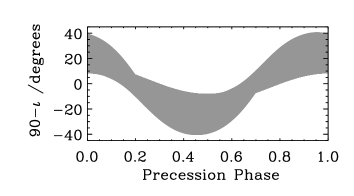
Figure 8: The accretion disc for the solution in Fig. 6 as seen from the compact object. The azimuth angle is equivalent to the precession phase. An observer at a high enough inclination $i$ sees the disc (grey areas) periodically crossing his line of sight to the central source.

An observer at an inclination $i$ close enough to $90\degr$ will see a succession of on-off states as the central source disappears behind the disc for certain phases. Observationally, the X-rays are not fully eclipsed during the off states, suggesting the emission region is extended, very much like accretion disc corona sources (Shakura et al. 1998). Further studies would need to assess whether such partial obscuration is compatible with the present model. Interestingly, the disc in a system seen edge-on need not always obscure the central source as can be seen from Fig. 8; but we would need to include the effects of a non-zero disc thickness to verify this.

Irradiation by the central source can heat the outer disc enough to quench the thermal-viscous instability. This is particularly important in low-mass X-ray binaries where the standard disc instability model without irradiation heating would predict many more unstable systems than actually observed (van Paradijs 1996). Irradiation is most important in the outer regions but these are completely self-shadowed in a flat disc (Dubus et al. 1999). If, however, the disc is warped then the outer regions may see the central source. Following Appendix A, the amount of irradiation received by each element in the disc is

$$F_{\rm irr}=\mbox{\boldmath$F$}\cdot\mbox{\boldmath$\hat{n}$}={\cal C}{L_{\star}\over{4\pi r^{2}}},$$ (56)

where we have defined ${\cal C}=\mbox{\boldmath$e$}_{r}\cdot\mbox{\boldmath$\hat{n}$}$ for the warped disc (Shakura & Sunyaev 1973; Dubus et al. 1999).

We show in Fig. 9 the variation of ${\cal C}$ in the disc. Dark areas are able to intercept a large fraction of the flux from the central source while white areas intercept little, or none if they are shadowed. The strongly irradiated regions form a two-armed spiral, although it should be understood that the re-emitted radiation from the two arms would be emitted on opposite sides of the disc. The average value of ${\cal C}$ over an annulus, taking self-shadowing into account, can be integrated like the radiation torque and this is shown in Fig. 10. In most of the outer region ${\cal C}$ is quite important ($\sim 0.1$) and even a large albedo (the fraction of the flux that is scattered) would not prevent significant heating of the outer disc. For a solution very close to the stability limit and thus corresponding to a much smaller tilt (about 2°), we find ${\cal C}\sim 5\cdot 10^{-3}$. Dubus et al. (1999) found that values of ${\cal C}$ of the order of $10^{-3}$ would be sufficient to heat the disc significantly and stabilize it against the thermal-viscous instability. A warp can easily provide such values of ${\cal C}$ even with a significant albedo. Taking the variations of $H/r$ into account would probably not change these conclusions: $H/r$ would be expected to increase with radius, albeit with some variations due to the warping (equation 43 of Ogilvie 2000), so that even a partially shadowed outer disc would see enough of the X-ray flux.

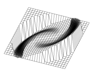
Figure 9: Another view of the stable, steadily precessing disc shown in Fig. 6. The grey-scale shows variations of the coefficient $\cal C$. The regions intercepting a large fraction of the flux are dark while those that intercept little or none (shadowed) appear white. Re-emission from the two arms occurs on opposite sides of the disc.

Figure 10: Average value of $\cal C$ (see Fig. 9) as a function of $r$, taking self-shadowing into account.

While X-ray irradiation appears important for all low-mass X-ray binaries (van Paradijs & McClintock 1994), only a fraction would be expected to be unstable to radiation-driven warping (Section 5.1). If warping is to explain how the outer disc can intercept the X-ray flux in all X-ray binaries then the warp must be produced differently (e.g. winds, Schandl & Meyer 1994; magnetic fields, although this may only work close to the magnetosphere, Lai 1999). The resulting disc will probably also be able to intercept a large fraction of the flux. Warping might have interesting consequences for Doppler tomography and eclipse mapping: if irradiation heating dominates, the emission from the disc is clearly asymmetric (Fig. 9; see also Still et al. 1997, where a search for such features is attempted for Her X-1); viscous heating would also result in asymmetric emission since it is significantly larger where the disc bends most (equation 44 of Ogilvie 2000).

5.5 Uncertainties and neglected effects

Our model rests on a number of assumptions and simplifications. Some of these may have affected our conclusions and we list them here as suggestions for future investigations.

1. Regarding the hydrodynamics of the warped disc, the principal uncertainty is the modelling of the turbulent stress. Although our results here favour a viscosity parameter $\alpha\ga 0.1$, this depends on our assumption that the underlying effective viscous process is isotropic. This difficult issue can be addressed only through numerical simulations of the turbulence (Torkelsson et al. 2000).

2. Although studying the dynamical effects of radiation, we have not taken into account the thermal effects of one-sided irradiation on the vertical structure of the disc. This has been considered by Ogilvie (2000) and could result in a fractional correction to equation (9).

3. In our treatment of irradiation and self-shadowing, we neglected the non-zero thickness of the disc.

4. Our treatment of mass input to the warped disc is admittedly oversimplified (Section 2.2.2).

5. The correct inner boundary condition for different central objects is debatable (Section 2.2.3).

6 Conclusion

We have studied the radiation-driven warping of accretion discs in X-ray binaries. The latest evolutionary equations were adopted, which extend the classical alpha theory to time-dependent thin discs with non-linear warps (Ogilvie 2000). We have also developed accurate, analytical expressions for the tidal torque and the radiation torque, including self-shadowing, that can be easily implemented in numerical calculations.

1. Using the complete set of equations, we re-examined the stability of discs to radiation-driven warping. We found that the critical binary separation is within an order of magnitude of the approximate criterion given by Pringle (1996) if the ratio of effective viscosities $\eta$ is given by equation (42).

2. Only the low-mass X-ray binaries with the longest orbital periods ($P_{\rm orb}\ga 1$d) are likely to be unstable to radiation-driven warping. This could explain the unusual outburst light-curves of the long-period soft X-ray transients. The disc-fed high-mass X-ray binaries are more likely to be unstable.

3. We solved directly for several branches of non-linear solutions representing steadily precessing warped discs. We studied the stability of these branches to further perturbations and found that typically only one branch is stable, and that only in a limited range of parameters. In this case, the precession is usually retrograde.

4. Discs that are beyond this range of parameters will probably show quasi-periodic or chaotic behaviour.

5. For $q\la 0.2$, the radiation-driven instability may produce progradely precessing warped discs.

6. There may exist a certain range of parameters (the ‘indeterminate instability zone’) for which a disc might cycle between being warped and being flat.

7. Our results are sensitive to assumptions concerning the effective viscosity of the disc. If the turbulence acts on internal shearing motions similarly to an isotropic effective viscosity, then values of $\alpha$ exceeding $0.1$, and preferably closer to $0.3$, are required.

Further studies should consider individual systems, including the correct tidal torque on a case-by-case basis, and should make a more detailed comparison with observations. For systems in which periodic behaviour is not indicated, a time-dependent method should be used to model their variability.

The present results confirm the conclusions of exploratory calculations by Wijers & Pringle (1999). Our methods, which are based on solving only ordinary differential equations, should be seen as complementary to their time-dependent numerical approach. High-precision solutions can be obtained rapidly using our approach, and traced throughout the parameter space, but the non-linear dynamics can only be followed up to the point at which the steadily precessing discs become unstable to further perturbations.

We find that showing the binary separation as a function of the mass ratio can be a powerful tool to discuss the behaviour of X-ray binaries with respect to radiation-driven warping (Fig. 7). For the systems selected, there is a very persuasive consistency between the model and the observations: for instance, Her X-1, SS 433 and LMC X-4 are very well explained by stable steadily precessing discs. However, most long-term variabilities observed in low-mass X-ray binaries cannot be associated with a radiatively-driven warped disc and might be due to modulations of the accretion rate. If warps are found to be ubiquitous in low-mass X-ray binaries, then it is likely that other driving mechanisms are at work.

Appendix A Radiation torque

In this section we derive an analytical expression for the radiation torque density $\mbox{\boldmath$T$}_{\rm rad}$. Our discussion is based largely on the analysis of Pringle (1996).

A.1 Geometrical considerations

Consider the disc to be composed of a sequence of concentric circular rings. The unit tilt vector $\mbox{\boldmath$l$}(r,t)$ of the rings varies continuously with radius $r$ and time $t$. In the notation of Ogilvie (1999),

$$\mbox{\boldmath$l$}=(\sin\beta\cos\gamma,\sin\beta\sin\gamma,\cos\beta),$$ (57)

where $\beta(r,t)$ and $\gamma(r,t)$ are the Euler angles of the tilt vector with respect to a fixed Cartesian coordinate system $(x,y,z)$. Introduce the dimensionless complex variable

$$\psi=|\psi|\,{\rm e}^{{\rm i}\chi}=r\left({{\partial\beta}\over{\partial r}}+{\rm i}{{\partial\gamma}\over{\partial r}}\sin\beta\right).$$ (58)

Then

$$|\psi|=\left|{{\partial\mbox{\boldmath$l$}}\over{\partial\ln r}}\right|$$ (59)

is a measure of the amplitude of the warp. In particular,

$$r{{\partial\mbox{\boldmath$l$}}\over{\partial r}}=|\psi|\left[\matrix{\cos\beta\cos\gamma\cos\chi-\sin\gamma\sin\chi\cr\cos\beta\sin\gamma\cos\chi+\cos\gamma\sin\chi\cr-\sin\beta\cos\chi}\right],$$ (60)

$$r\mbox{\boldmath$l$}\times{{\partial\mbox{\boldmath$l$}}\over{\partial r}}=|\psi|\left[\matrix{-\cos\beta\cos\gamma\sin\chi-\sin\gamma\cos\chi\cr-\cos\beta\sin\gamma\sin\chi+\cos\gamma\cos\chi\cr\sin\beta\sin\chi}\right].$$ (61)

The position vector of a point on the ring of radius $r$ is $\mbox{\boldmath$r$}=r\,\mbox{\boldmath$e$}_{r}$, where (equation 7 of Ogilvie 1999, with $\theta=\pi/2$)

$$\mbox{\boldmath$e$}_{r}=\left[\matrix{\cos\beta\cos\gamma\cos\phi-\sin\gamma\sin\phi\cr\cos\beta\sin\gamma\cos\phi+\cos\gamma\sin\phi\cr-\sin\beta\cos\phi}\right]$$ (62)

is the radial unit vector and $\phi$ the azimuth on the ring. Note that $\mbox{\boldmath$l$}\cdot\mbox{\boldmath$e$}_{r}=0$, since points on the ring lie in the plane that passes through the origin and is orthogonal to $l$. Now $(r,\phi)$ are (in general) non-orthogonal coordinates on the surface of the disc. The element of surface area is

$${\rm d}\mbox{\boldmath$S$}=\left({{\partial\mbox{\boldmath$r$}}\over{\partial r}}\,{\rm d}r\right)\times\left({{\partial\mbox{\boldmath$r$}}\over{\partial\phi}}\,{\rm d}\phi\right),$$ (63)

which simplifies to

$${\rm d}\mbox{\boldmath$S$}=\left[\mbox{\boldmath$l$}+|\psi|\cos(\phi-\chi)\,\mbox{\boldmath$e$}_{r}\right]r\,{\rm d}r\,{\rm d}\phi.$$ (64)

The unit normal to the surface is then

$$\mbox{\boldmath$\hat{n}$}=\left[1+|\psi|^{2}\cos^{2}(\phi-\chi)\right]^{-1/2}\left[\mbox{\boldmath$l$}+|\psi|\cos(\phi-\chi)\,\mbox{\boldmath$e$}_{r}\right].$$ (65)

A.2 Radiation

Let the disc be illuminated by isotropic radiation from the central source, of luminosity $L_{\star}$. Then the energy flux is

$$\mbox{\boldmath$F$}={{L_{\star}}\over{4\pi r^{2}}}\,\mbox{\boldmath$e$}_{r},$$ (66)

except in regions of shadow. The power incident on an illuminated surface element ${\rm d}\mbox{\boldmath$S$}$ is

$${\rm d}P=|\mbox{\boldmath$F$}\cdot{\rm d}\mbox{\boldmath$S$}|={{L_{\star}}\over{4\pi r^{2}}}|\psi||\cos(\phi-\chi)|\,r\,{\rm d}r\,{\rm d}\phi.$$ (67)

Assume that the element absorbs the incident radiation and re-radiates it immediately and uniformly from the same side. Since the incident radiation is parallel to the radius vector, the element receives no torque from the absorption process. However, it receives a reaction force

$${\rm d}\mbox{\boldmath$F$}=-{{2}\over{3}}{{{\rm d}P}\over{c}}\,(\pm\mbox{\boldmath$\hat{n}$})$$ (68)

from the re-radiation process, where $(\pm\mbox{\boldmath$\hat{n}$})$ is the normal pointing away from the disc on the side that received the radiation. The correct sign is determined from the condition $\mbox{\boldmath$e$}_{r}\cdot(\pm\mbox{\boldmath$\hat{n}$})<0$, which implies

$${\rm d}\mbox{\boldmath$F$}={{L_{\star}}\over{6\pi r^{2}c}}|\psi|\cos(\phi-\chi)\,\mbox{\boldmath$\hat{n}$}\,r\,{\rm d}r\,{\rm d}\phi.$$ (69)

The corresponding torque is

$$\mbox{\boldmath$r$}\times{\rm d}\mbox{\boldmath$F$}={{L_{\star}}\over{6\pi rc}}q(1+q^{2})^{-1/2}(\mbox{\boldmath$e$}_{r}\times\mbox{\boldmath$l$})\,r\,{\rm d}r\,{\rm d}\phi,$$ (70)

where $q=|\psi|\cos(\phi-\chi)$. The radiation torque density $\mbox{\boldmath$T$}_{\rm rad}(r,t)$ is defined such that $2\pi\mbox{\boldmath$T$}_{\rm rad}\,r\,{\rm d}r$ is the torque acting on a ring of radius $r$ and of infinitesimal radial extent ${\rm d}r$. Therefore

$$\mbox{\boldmath$T$}_{\rm rad}=-{{L_{\star}}\over{12\pi rc}}\,\mbox{\boldmath$l$}\times\mbox{\boldmath$a$},$$ (71)

where

$$\mbox{\boldmath$a$}={{1}\over{\pi}}\int q(1+q^{2})^{-1/2}\,\mbox{\boldmath$e$}_{r}\,{\rm d}\phi$$ (72)

is a dimensionless integral.

Assume at this stage that there is no self-shadowing, so that the integral is taken from $\phi=0$ to $\phi=2\pi$, or, equivalently, from $\phi=\chi$ to $\phi=\chi+2\pi$. Since $\mbox{\boldmath$e$}_{r}$ is a linear combination of $\cos\phi$ and $\sin\phi$, the basic integrals required to compute $a$ are

$${{1}\over{\pi}}\int_{0}^{2\pi}(1+x^{2}\cos^{2}\alpha)^{-1/2}\cos^{2}\alpha\,{\rm d}\alpha = f(x),$$

$${{1}\over{\pi}}\int_{0}^{2\pi}(1+x^{2}\cos^{2}\alpha)^{-1/2}\cos\alpha\sin\alpha\,{\rm d}\alpha = 0,$$ (73)

where

$$f(x)={{4}\over{\pi x^{2}(1+x^{2})^{1/2}}}\left[(1+x^{2})E(k)-K(k)\right].$$ (74)

Here

$$K(k) = \int_{0}^{\pi/2}(1-k^{2}\sin^{2}\alpha)^{-1/2}\,{\rm d}\alpha,$$

$$E(k) = \int_{0}^{\pi/2}(1-k^{2}\sin^{2}\alpha)^{1/2}\,{\rm d}\alpha,$$ (75)

are the complete elliptic integrals of the first and second kinds, respectively, of modulus $k=x/(1+x^{2})^{1/2}$. Thus

$${{1}\over{\pi}}\int_{0}^{2\pi}q(1+q^{2})^{-1/2}\cos\phi\,{\rm d}\phi = |\psi|\cos\chi\,f(|\psi|),$$

$${{1}\over{\pi}}\int_{0}^{2\pi}q(1+q^{2})^{-1/2}\sin\phi\,{\rm d}\phi = |\psi|\sin\chi\,f(|\psi|),$$ (76)

and so

$$\mbox{\boldmath$a$}=f(|\psi|)\,r{{\partial\mbox{\boldmath$l$}}\over{\partial r}}.$$ (77)

We obtain finally

$$\mbox{\boldmath$T$}_{\rm rad}=-{{L_{\star}}\over{12\pi c}}f(|\psi|)\,\mbox{\boldmath$l$}\times{{\partial\mbox{\boldmath$l$}}\over{\partial r}}.$$ (78)

The factor $f(|\psi|)$ reduces the effectiveness of the radiation torque when the disc is significantly warped. It is a monotonically decreasing function of its argument, with $f(0)=1$ and $f(x)\sim 4/(\pi x)$ as $x\to\infty$. It has the Taylor series

$$f(x)=1-{{3}\over{8}}x^{2}+{{15}\over{64}}x^{4}-{{175}\over{1024}}x^{6}+O(x^{8}).$$ (79)

A.3 Self-shadowing

Consider the ring of radius $r$, with tilt vector $l$, and consider an arbitrary ring of smaller radius $\hat{r}<r$, with tilt vector $\mbox{\boldmath$\hat{l}$}\neq\mbox{\boldmath$l$}$. The smaller ring obscures the radiation in the plane orthogonal to $\hat{l}$ and casts shadows at two diametrically opposite points on the larger ring. These points lie in the plane orthogonal to $\hat{l}$ and are therefore defined by $\mbox{\boldmath$r$}\cdot\mbox{\boldmath$\hat{l}$}=0$. This determines their azimuth $\phi_{\rm s}$ according to

$$\tan\phi_{\rm s}={{\hat{\ell}_{x}\cos\beta\cos\gamma+\hat{\ell}_{y}\cos\beta\sin\gamma-\hat{\ell}_{z}\sin\beta}\over{\hat{\ell}_{x}\sin\gamma-\hat{\ell}_{y}\cos\gamma}}.$$ (80)

However, it is more convenient to measure the azimuth with respect to the angle $\chi$, i.e. $\theta=\phi-\chi$. We then find the covariant expression

$$\tan\theta_{\rm s}=-\left(\mbox{\boldmath$\hat{l}$}\cdot{{\partial\mbox{\boldmath$l$}}\over{\partial r}}\right)\bigg{/}\left(\mbox{\boldmath$\hat{l}$}\cdot\mbox{\boldmath$l$}\times{{\partial\mbox{\boldmath$l$}}\over{\partial r}}\right).$$ (81)

Note that $\theta_{\rm s}$ is not uniquely defined since any multiple of $\pi$ may be added to it. Consider a single branch, therefore, and follow $\theta_{\rm s}$ continuously as $\hat{r}$ varies from the inner radius of the disc up to $r$. Let $\theta_{\rm min}$ and $\theta_{\rm max}$ denote the minimum and maximum values obtained. Then the shadow on the ring considered consists of the two segments $\theta_{\rm min}<\theta<\theta_{\rm max}$ and $\theta_{\rm min}+\pi<\theta<\theta_{\rm max}+\pi$. If these overlap (i.e. if $\theta_{\rm max}-\theta_{\rm min}>\pi$), the ring is completely shadowed and the radiation torque is zero. Otherwise, we must reconsider the integral $a$ in the form

$$a = {{1}\over{\pi}}\int_{\theta_{\rm max}}^{\theta_{\rm min}+\pi}q(1+q^{2})^{-1/2}\,\mbox{\boldmath$e$}_{r}\,{\rm d}\theta$$ (82)

$$+{{1}\over{\pi}}\int_{\theta_{\rm max}+\pi}^{\theta_{\rm min}+2\pi}q(1+q^{2})^{-1/2}\,\mbox{\boldmath$e$}_{r}\,{\rm d}\theta$$

$$= {{2}\over{\pi}}\int_{\theta_{\rm max}}^{\theta_{\rm min}+\pi}q(1+q^{2})^{-1/2}\,\mbox{\boldmath$e$}_{r}\,{\rm d}\theta.$$

Now the basic integrals required are

$${{2}\over{\pi}}\int_{0}^{\theta}(1+x^{2}\cos^{2}\alpha)^{-1/2}\cos^{2}\alpha\,{\rm d}\alpha = g_{1}(\theta,x),$$

$${{2}\over{\pi}}\int_{0}^{\theta}(1+x^{2}\cos^{2}\alpha)^{-1/2}\cos\alpha\sin\alpha\,{\rm d}\alpha = g_{2}(\theta,x),$$ (83)

where

$$g_{1}(\theta,x) = {{2}\over{\pi x^{2}(1+x^{2})^{1/2}}}\left[(1+x^{2})E(\theta,k)-F(\theta,k)\right],$$

$$g_{2}(\theta,x) = {{2}\over{\pi x^{2}}}\left[(1+x^{2})^{1/2}-(1+x^{2}\cos^{2}\theta)^{1/2}\right].$$ (84)

Here

$$F(\theta,k) = \int_{0}^{\theta}(1-k^{2}\sin^{2}\alpha)^{-1/2}\,{\rm d}\alpha,$$

$$E(\theta,k) = \int_{0}^{\theta}(1-k^{2}\sin^{2}\alpha)^{1/2}\,{\rm d}\alpha,$$ (85)

are the incomplete elliptic integrals of the first and second kinds, respectively, again of modulus $k=x/(1+x^{2})^{1/2}$. Thus

$$a = \left[g_{1}(\theta_{\rm min}+\pi,|\psi|)-g_{1}(\theta_{\rm max},|\psi|)\right]r{{\partial\mbox{\boldmath$l$}}\over{\partial r}}$$ (86)

$$+\left[g_{2}(\theta_{\rm min}+\pi,|\psi|)-g_{2}(\theta_{\rm max},|\psi|)\right]r\mbox{\boldmath$l$}\times{{\partial\mbox{\boldmath$l$}}\over{\partial r}}.$$

Noting that $g_{1}(\theta+\pi,x)-g_{1}(\theta,x)=f(x)$ and $g_{2}(\theta+\pi,x)-g_{2}(\theta,x)=0$, we confirm that the previous result is recovered in the limit $\theta_{\rm max}-\theta_{\rm min}\to 0$.

The elliptic integrals can be evaluated quickly and accurately using Carlson’s algorithms (see Press et al. 1992).

A.4 Scattering

In reality, when X-rays from the central source are incident on the disc, a significant fraction of the photons are scattered from the surface rather than absorbed. Wijers & Pringle (1999) suggested that this X-ray albedo might reduce the effectiveness of the radiation torque. However, we consider that the torque due to scattered radiation will be very similar to that due to radiation that is absorbed and re-emitted, because in each case the photons leaving the disc have the same total energy flux as the incident radiation flux, and the distribution of momenta of those photons is peaked around the normal to the disc surface. The non-isotropy of the Thomson cross-section is quickly lost after a few scatterings and the photons finally leaving the disc have paths almost perpendicular to the surface. The torque due to scattered radiation could only be much smaller if the net effect of the scattering process was to divert the momenta of the photons through a small angle, which would require specular reflection from a slightly warped surface. In conclusion, the albedo of the disc is probably irrelevant to radiation-driven warping.

Appendix B Tidal torque

Assume that the companion star may be treated as a point mass $M_{2}$ describing a circular orbit in the $xy$-plane. The position vector of the companion star is then

$$\mbox{\boldmath$r$}_{2}=r_{\rm b}(\cos\Omega_{\rm b}t,\sin\Omega_{\rm b}t,0),$$ (87)

The time-averaged gravitational potential due to the companion star is

$$\Phi_{2}(\mbox{\boldmath$r$})=-{{GM_{2}}\over{2\pi}}\int_{0}^{2\pi}{{1}\over{|\mbox{\boldmath$r$}-\mbox{\boldmath$r$}_{2}|}}\,{\rm d}(\Omega_{\rm b}t).$$ (88)

For $|\mbox{\boldmath$r$}|<|\mbox{\boldmath$r$}_{2}|$ we obtain the expansion

$$\Phi_{2}=-{{GM_{2}}\over{r_{\rm b}}}\left[1+{{(s^{2}-2z^{2})}\over{4r_{\rm b}^{2}}}+{{3(3s^{4}-24s^{2}z^{2}+8z^{4})}\over{64r_{\rm b}^{4}}}\right.$$ (89)

$$\left.+{{5(5s^{6}-90s^{4}z^{2}+120s^{2}z^{4}-16z^{6})}\over{256r_{\rm b}^{6}}}+\cdots\right],$$

where $s^{2}=x^{2}+y^{2}$.

Consider a circular ring of radius $r$, centred on the origin and tilted at an angle $\beta$ to the binary plane. Owing to the axial symmetry of $\Phi_{2}$, we may take the tilt vector to be

$$\mbox{\boldmath$l$}=(\sin\beta,0,\cos\beta)$$ (90)

without loss of generality. The position vector of a point on the ring is then

$$\mbox{\boldmath$r$}=r(\cos\beta\cos\phi,\sin\phi,-\sin\beta\cos\phi),$$ (91)

where $\phi$ is the azimuth on the ring. It is clear from the symmetry of the situation that the net torque on the ring has only a $y$-component. Now the $y$-component of the torque per unit mass is

$$t_{y}=-z{{\partial\Phi_{2}}\over{\partial x}}+x{{\partial\Phi_{2}}\over{\partial z}}.$$ (92)

When averaged over $\phi$ this gives

$$\langle t_{y}\rangle=-{{GM_{2}}\over{r_{\rm b}}}\left[{{3r^{2}}\over{8r_{\rm b}^{2}}}\sin 2\beta+{{45r^{4}}\over{1024r_{\rm b}^{4}}}(2\sin 2\beta+7\sin 4\beta)\right.$$ (93)

$$\left.+{{525r^{6}}\over{65536r_{\rm b}^{6}}}(5\sin 2\beta+12\sin 4\beta+33\sin 6\beta)+\cdots\right].$$

The tidal torque density $\mbox{\boldmath$T$}_{\rm tide}$ is obtained by multiplying by the surface density $\Sigma$. Noting that $\mbox{\boldmath$e$}_{z}\cdot\mbox{\boldmath$l$}=\cos\beta$ and $\mbox{\boldmath$e$}_{z}\times\mbox{\boldmath$l$}=\sin\beta\,\mbox{\boldmath$e$}_{y}$, we may write $\mbox{\boldmath$T$}_{\rm tide}$ in the covariant form

$$\mbox{\boldmath$T$}_{\rm tide}=-{{3GM_{2}\Sigma r^{2}}\over{4r_{\rm b}^{3}}}(\mbox{\boldmath$e$}_{z}\cdot\mbox{\boldmath$l$})(\mbox{\boldmath$e$}_{z}\times\mbox{\boldmath$l$})$$ (94)

$$\times\left\{1+{{15}\over{32}}\left({{r}\over{r_{\rm b}}}\right)^{2}\left[7(\mbox{\boldmath$e$}_{z}\cdot\mbox{\boldmath$l$})^{2}-3\right]\right.$$

$$\left.+{{175}\over{512}}\left({{r}\over{r_{\rm b}}}\right)^{4}\left[33(\mbox{\boldmath$e$}_{z}\cdot\mbox{\boldmath$l$})^{4}-30(\mbox{\boldmath$e$}_{z}\cdot\mbox{\boldmath$l$})^{2}+5\right]+\cdots\right\}.$$

This series converges quite rapidly. The magnitude of the fourth term (not shown) in the series in braces is less than $0.0027$ when $r/r_{\rm b}<0.3$. This suggests that the series as truncated above is accurate to within a fraction of a percent for all the calculations in this paper. Of course, higher-order terms can easily be calculated if desired.

If the torque is not averaged over the binary orbital period, it is found to contain an additional, oscillatory component with frequency $2\Omega_{\rm b}$. The oscillatory torque causes a small wobbling motion but is unlikely to be important otherwise, except in very thick discs, or discs much smaller than the standard tidal truncation radius (Lubow & Ogilvie 2000).

References

- [] Abramowicz M., Brandenburg A., Lasota J.-P., 1996, MNRAS, 281, L21
- [] Armitage P. J., Livio M., 1998, ApJ, 493, 898
- [] Balbus S. A., Hawley J. F., 1998, Rev. Mod. Phys., 70, 1
- [] Bate M. R., Bonnell I. A., Clarke C. J., Lubow S. H., Ogilvie G. I., Pringle J. E., Tout C. A., 2000, MNRAS, in press
- [] Bildsten L., et al., 1997, ApJSS, 113, 367
- [] Blum S., Kraus O., 2000, ApJ, 529, 968
- [] Brandenburg A., 1998, in Abramowicz M. A., Björnsson G., Pringle J. E., eds, Theory of Black Hole Accretion Discs, Cambridge Univ. Press, Cambridge, p. 61
- [] Brocksopp C., Fender R. P., Larionov V., Lyuty V. M., Tarasov A. E., Pooley G. G., Paciesas W. S., Roche P., 1999, MNRAS, 309, 1063
- [] Cannizzo J. K., 1998, in Wild Stars in the Old West, ASP Conf. Ser. 137, 308
- [] Chen W., Shrader C. R., Livio M., 1997, ApJ, 491, 312
- [] Cheng F. H., Vrtilek S. D., Raymond J. C., 1995, ApJ, 452, 825
- [] Choi C. S., Nagase F., Makino F. Dotani T., Min K. W., 1994, ApJ, 422, 799
- [] Corbet R. H. D., Peele A. G., 1997, in Matsuoka M., Kawai N., eds, All-Sky X-Ray Observations in the Next Decade, RIKEN, Japan, p.75
- [] Dubus G., Charles P. A., Long K. S., Hakala P. J., 1997, ApJ, 490, L47
- [] Dubus G., Lasota J. P., Hameury J. M., Charles P.A., 1999, 303, 139
- [] Esin A. A., Lasota J. P., Hynes R. I., 2000, A&A, 354, 987
- [] Flannery B. P., 1975, MNRAS, 170, 325
- [] Gammie C. F., 1999, ApJ, 522, L57
- [] Gammie C. F., Goodman J., Ogilvie G. I., 2000, MNRAS, in press
- [] Gerend D., Boynton P. E., 1976, ApJ, 209, 562
- [] Hakala P. J., Muhli P., Dubus G. 1999, MNRAS, 306, 701
- [] Hawley J. F., 2000, ApJ, 528, 462
- [] Hatchett S. P. Begelman M. C., Sarazin C. L., 1981, ApJ, 247, 677
- [] Heemskerk M. H. M., van Paradijs J., 1989, A&A, 223, 154
- [] Hjellming R. M., Johnston K. J., 1981, ApJ, 246, L141
- [] Ilovaisky S. A., 1984, Phys. S., 7, 78
- [] Iooss G., Joseph D. D., 1980, Elementary Stability and Bifurcation Theory, Springer, New York
- [] Iping R. C., Petterson J. A., 1990, A&A, 239, 221
- [] Johnston H. M., Fender R., Wu K., 1999, MNRAS, 308, 415
- [] Katz J. I., 1973, Nat, 246, 87
- [] Krolik J. H., 1999, ApJ, 515, L73
- [] Kuulkers E., van der Klis M., Vaughan B. A., 1996, A&A, 311, 197
- [] Kuulkers E., in’t Zand J. J. M., Cornelisse R., et al., 2000, A&A, 358, 993
- [] Lai D., 1999, ApJ, 524, 1030
- [] Larwood J. D., Nelson R. P., Papaloizou J. C. B., Terquem C., 1996, MNRAS, 282, 597
- [] Leibowitz E. M., 1984, MNRAS, 210, 279
- [] Lubow S. H., Shu F. H., 1975, ApJ, 198, 383
- [] Lubow S. H., Ogilvie G. I., 2000, ApJ, 538, 326
- [] Maloney P. R., Begelman M. C., 1997, ApJ, 491, L43
- [] Maloney P. R., Begelman M. C., Nowak M. A., 1998, ApJ, 504, 77
- [] Maloney P. R., Begelman M. C., Pringle J. E., 1996, ApJ, 472, 582
- [] Margon B., 1984, ARA&A, 22, 507
- [] Nowak M. A., Wilms J., 1999a, ApJ, 522, 476
- [] Nowak M. A., Wilms J. , Vaughan B. A., Dove J. B., Begelman M. C., 1999b, ApJ, 515, 726
- [] Ogilvie G. I., 1999, MNRAS, 304, 557
- [] Ogilvie G. I., 2000, MNRAS, in press
- [] Paczyński B., 1977, ApJ, 216, 822
- [] Papaloizou J. C. B., Lin D. N. C., 1995, ApJ, 438, 841
- [] Papaloizou J. C. B., Pringle J. E., 1977, MNRAS, 181, 441
- [] Papaloizou J. C. B., Pringle J. E., 1983, MNRAS, 202, 1181
- [] van Paradijs J., 1996, ApJ, 464, L139
- [] van Paradijs J., McClintock J. E., 1994, A&A, 290, 133
- [] Paul B., Kitamoto S., Makino F., 2000, ApJ, 528, 410
- [] Petterson J. A., 1975, ApJ, 201, L61
- [] Petterson J. A., 1977, ApJ, 216, 827
- [] Petterson J. A., 1978, ApJ, 224, 628
- [] Press W. H., Teukolsky S. A., Vetterling W. T., Flannery B. P., 1992, Numerical Recipes in Fortran, 2nd ed., Cambridge Univ. Press, Cambridge
- [] Priedhorsky W. C., Terrell J., 1983, ApJ, 273, 709
- [] Priedhorsky W. C., Holt S. S., 1987, Space Sci. Rev., 45, 291
- [] Pringle J. E., 1992, MNRAS, 258, 811
- [] Pringle J. E., 1996, MNRAS, 281, 357
- [] Reynolds A. P., Quaintrell H., Still M. D., Roche P., Chakrabarty D., Levine S. E., 1997, MNRAS, 288, 43
- [] Schandl S., 1996, A&A, 307, 95
- [] Schandl S., Meyer F., 1994, A&A, 289, 149
- [] Schwarzenberg-Czerny A., 1992, A&A, 260, 268
- [] Scott D. M., Leahy D. A., Wilson R. B., 2000, ApJ, submitted (astro-ph/0002327)
- [] Shakura N. I., Sunyaev R. A., 1973, A&A, 24, 337
- [] Shakura N. I., Ketsaris N. A., Prokhorov M. E., Postnov K. A., 1998, MNRAS, 300, 992
- [] Smak J., 1999, Acta Astronomica, 49, 391
- [] Smale A. P., Lochner J. C., 1992, ApJ, 395, 582
- [] Still M. D., Quaintrell H., Roche P. D, Reynolds A. P., 1997, MNRAS, 292, 52
- [] Thorne K. S., 1974, ApJ, 191, 507
- [] Torkelsson U., Ogilvie G. I., Brandenburg A., Pringle J. E., Nordlund Å., Stein R. F., 2000, MNRAS, in press
- [] Tsunemi H., Kitamoto S., Tamura K., 1996, ApJ, 456, 316
- [] White N. E., Nagase F., Parmar A. N., 1995, in Lewin W. H. G., van Paradijs J., van den Heuvel E. P. J., eds, X-ray Binaries, Cambridge Univ. Press, Cambridge, p. 1
- [] Wijers R. A. M. J., Pringle J. E., 1999, MNRAS, 308, 207
- [] Wijnands R. A. D., Kuulkers E., Smale A. P., 1996, ApJ, 473, L45
- [] Wilms J., Nowak M. A., Pottschmidt K. et al., 2000, ApJ, submitted (astro-ph/0005489)
- [] Wojdowski P., Clark G. W., Levine A. M., Woo J. W., Zhang S. N., 1998, ApJ, 502, 253
- [] Woo J. W., Clark G. W., Levine A. M., 1995, ApJ, 449, 880