A Complete Survey of Case A Binary Evolution with Comparison to Observed Algol-type Systems

Abstract

We undertake a comparison of observed Algol-type binaries with a library of computed Case A binary evolution tracks. The library consists of 5500 binary tracks with various values of initial primary mass $M_{10}$, mass ratio $q_{0}$, and period $P_{0}$, designed to sample the phase-space of Case A binaries in the range $-0.10\leq\log M_{10}\leq 1.7$. Each binary is evolved using a standard code with the assumption that both total mass and orbital angular momentum are conserved. This code follows the evolution of both stars until the point where contact or reverse mass transfer occurs. The resulting binary tracks show a rich variety of behavior which we sort into several subclasses of Case A and Case B. We present the results of this classification, the final mass ratio and the fraction of time spent in Roche Lobe overflow for each binary system. The conservative assumption under which we created this library is expected to hold for a broad range of binaries, where both components have spectra in the range G$0$ to B$1$ and luminosity class III – V. We gather a list of relatively well-determined observed hot Algol-type binaries meeting this criterion, as well as a list of cooler Algol-type binaries where we expect significant dynamo-driven mass loss and angular momentum loss. We fit each observed binary to our library of tracks using a $\chi^{2}$-minimizing procedure. We find that the hot Algols display overall acceptable $\chi^{2}$, confirming the conservative assumption, while the cool Algols show much less acceptable $\chi^{2}$ suggesting the need for more free parameters, such as mass and angular momentum loss.

1 Introduction

Many binary stars are observed to be undergoing Roche-lobe overflow (RLOF), which is recognised as being a natural response to the fact that, for a binary of given separation, there is a critical maximum radius, the Roche-lobe radius, that a star cannot exceed without losing mass to its companion. There are many sub-types of stars undergoing RLOF, but we concentrate here on those which, like the prototype Algol, consist of (i) a lobe-filling, mass-losing star that is substantially above the main sequence, and (ii) a component which underfills its Roche lobe, and is usually nearer to, though still larger than, the main sequence. We concentrate on those (Case A) with short initial periods, the lower and upper period depending on the primary mass.

It is not difficult to evolve theoretically pairs of stars with a given initial primary mass $M_{10}$, initial mass ratio $q_{0}$ and initial orbital period $P_{0}$, and follow them into, and beyond, the stage of RLOF. However, such evolution is certainly affected by assumptions regarding both mass loss and angular momentum loss from the system as a whole. As a zero-order model it is commonly supposed that both total mass and orbital angular momentum are conserved, and we have computed conservative evolution for a large number of binary initial parameters: $37\times 10\times 15$ models with various $M_{10}$, $q_{0}$ and $P_{0}$. Most of the periods considered are appropriate to Case A, but some correspond to Case B.

There is plenty of evidence, both direct and indirect, that mass loss and/or angular momentum loss takes place in at least some systems. If mass escapes from the system as stellar wind, then it will also carry angular momentum away. Mass loss is observed fairly directly both in cool stars, where it appears to be driven by dynamo activity in their convective envelopes, and in hot stars, where radiation pressure in spectral lines may be the main driving force. Mass loss is also clearly evident in many stars of supergiant luminosity, across the whole range of spectral types; but we do not consider supergiants here. However there is a broad range of spectra, from about G0 to perhaps B1 and luminosity class III – V, where there is rather little evidence of significant mass loss, and where the conservative assumption may therefore be reasonable. We test this by comparing a selection of observed ‘hot Algols’ (having both spectra in this range) with theoretical conservative models, using a $\chi^{2}$ test. We find a reasonable agreement, especially if we exclude one system which is near the extreme of this temperature range. Comparing the same conservative models against some observed ‘cool Algols’ we find, as we expect, that the agreement is much poorer.

We have used a massively-parallel array, the Compaq Teracluster 2000 at LLNL, to evolve our data cube of models. This data cube covers the following ranges of initial primary mass $M_{10}$ (in solar units), initial mass ratio, defined by

$$q_{0}\equiv\frac{M_{10}}{M_{20}}>1\ ,$$ (1)

and initial period $P_{0}$:

$$\log M_{10}=-0.10,-0.05,\dots,1.7\ ,$$ (2a)

$$\log q_{0}=0.05,0.10,\dots,0.5\ ,$$ (2b)

$$\log(P_{0}/P_{ZAMS})=0.05,0.1,\dots,0.75\ .$$ (2c)

Here $P_{ZAMS}$, a function of $M_{10}$, is the period at which the initially more massive component would just fill its Roche lobe on the zero-age main sequence. We used the approximation

$$P_{ZAMS}\approx\frac{0.19M_{10}+0.47M_{10}^{2.33}}{1+1.18M_{10}^{2}}\ .$$ (3)

These initial periods cover Case A and a small part of Case B. We constructed such a ‘data cube’ with each of six metallicities ($Z=0.03,0.02,0.01,0.004,0.001,.0003$), and also, for $Z=0.02$ only, with three different assumptions about mass loss/angular momentum loss (in addition to the conservative assumption). We present here only the conservative, $Z=0.02$ data cube.

In §2, we discuss the numerical modelling and the physical assumptions that go into our data cube, and in §3 we discuss the results. We attempt to classify the results into a small number of sub-categories of Case A (and some analogues in Case B), depending for instance on whether the two components come into contact rapidly, slowly, or not at all after the start of RLOF, and (in the last case) on whether or not primary reaches a supernova before the secondary swells up enough to reach reverse RLOF. In §4 we discuss our attempts to fit several observed semidetached systems (Algols) with the theoretical models. We give our conclusions in §5.

We emphasise here that even if a particular Algol can be reasonably fitted by a conservative model, this does not prove that the evolution was conservative. Some models of non-conservation might lead to the same current parameters, starting from different initial conditions. Even if we had a mass loss/angular momentum loss model with no free parameters in it, we might still have ambiguity, partly because there are only six independent observational parameters (current $P,~{}M_{1},~{}M_{2},~{}R_{2},~{}T_{1},~{}T_{2}$) to be fitted by four theoretical parameters (age, and $P_{0},~{}M_{10},~{}q_{0}$), and partly because our data cube is still quite coarse even with 5550 models in it.

We also emphasise that throughout this paper we use suffixes 1 and 2 consistently to refer to the components with the greater and smaller initial mass respectively. This may seem unfortunate since observers normally call the currently hotter (and normally more massive) component the ‘primary’, at least in Algol systems. This component is the descendant of the originally less massive star. We do not think it would be helpful to interchange the suffices at the points in evolution where the ordering of the temperatures changes. However to avoid the most obvious possibility of confusion we do not use the terms ‘primary’ and ‘secondary’: instead we refer to the components as $*1$ (pronounced ’star one’) and $*2$, and keep these designations throughout their entire evolution. The mass ratio $q$ as defined in Equation 1 always starts off with $q_{0}>1$. After some RLOF it is commonly $<1$.

2 The Theoretical Data Cube

We used the stellar evolution code most recently described by Pols et al. (1995), based on the code of Eggleton (1971, 1972); Eggleton, Faulkner & Flannery (1973). This code is fully implicit in the composition equations as well as in the structure and the mesh-spacing equations. The implicit adaptive mesh is particularly useful for mass-transfer situations. In fact, it means that in a first approximation we do not have to do anything to the code to account for mass transfer, except replace a boundary condition $M(t)={\rm constant}$ by a condition which gives the mass-loss rate $\dot{M}$ as a function of stellar radius $R$ and Roche-lobe radius $R_{\rm L}$ (Tout & Eggleton, 1988).

We will not repeat here a description of the physical input (Pols et al. 1995). We have however included a simplistic model of convective overshooting (Schröder, Pols & Eggleton, 1997; Pols et al., 1997), based on a comparison of theoretical and observed non-interacting binaries. Other assumptions in the code are standard, and include the following: (a) the convective mixing of composition is treated as a diffusion equation, with diffusion coefficient a function of $\nabla_{r}-\nabla_{a}$ (Eggleton, 1972), and (b) because the mesh is fully adaptive, i.e. non-Lagrangian, an upstream advection term is needed in all time derivatives (Eggleton, 1971). The former ensures that any convection zones satisfy the K. Schwarzschild convection criterion ($\nabla_{\rm r}\approx\nabla_{\rm a}$) and simultaneously that any semiconvection zones that may arise satisfy the M. Schwarzschild condition (Schwarzschild & Härm, 1958) and are dealt with automatically, without extra code; the latter ensures that any evolutionary stage involving thin burning shells is computed very efficiently.

Regarding situations specific to binaries, we make the following assumptions:

1. The star is still treated as spherically symmetric, the radial coordinate $r$ being the volume-radius of an equipotential surface. The gravity at effective radius $r$ is reduced by a factor dependent on angular velocity:

   $$g=\frac{Gm}{r^{2}}\left(1-\frac{2\Omega^{2}r^{3}}{3Gm}\right)\ ,$$ (4)

   where $m$ is the mass within an equipotential of volume-radius $r$ and $\Omega$ is the angular velocity of the star, assumed corotating with the binary.

2. Mass transfer from a star that overfills its Roche lobe is treated as spherically symmetric, and governed by the boundary condition

   $$\begin{array}[]{cc}\dot{M}&=-C\{\log(R/R_{\rm L})^{3}\},\ \ R>R_{\rm L}\\ &=0,\ \ R<R_{\rm L}\end{array}$$ (5)

   where $C=500\thinspace M_{\odot}/$yr. Thus a transfer rate of $5\times 10^{-7}M_{\odot}/$yr corresponds to an overfill of 0.1%. We only do this for $*1$. There inevitably comes a point in evolution when $*2$ fills its own Roche lobe, but this is usually either (a) while $*1$ already fills its own lobe, so that the binary comes into contact – for the present, we stop evolution at this point; or (b) when $*1$ has evolved to a late and relatively compact state of low mass, and $*2$ has grown to a very large radius. In the latter case the mass ratio is very small ($q\lesssim 0.2$). Therefore the mass transfer can be expected to be rapid, and unstable on a short (hydrodynamical) timescale. We expect common-envelope evolution beyond this point (Paczyński, 1976), and so we stop evolution at this point, also.

3. It is assumed that the matter which leaves $*1$ is accreted in a spherically symmetric manner at the surface of $*2$, with entropy and temperature equal to the surface values of $*2$. Thus no model is incorporated for the temperature/entropy budget of the material during transfer. This may seem potentially serious, but when most of the mass is transferred on a nuclear timescale it should not be important.

4. The composition of accreting material on $*2$ is assumed to be the same as that of material already just below the surface of $*2$, rather than (as it should be) of the material leaving $*1$. This is just done for convenience, and is only significantly in error at a fairly late stage in mass transfer. The observed Algols that we make comparison with are probably not at such late stages.

5. On a somewhat technical level, the implementation of Equations 4 and  5 numerically within the framework of a fully implicit and adaptive code means that it is desirable, though possibly not essential, to introduce an extra equation into the usual set of difference equations – for the structure, composition and mesh-distribution variables – that are solved for by Newton-Raphson iteration. This is because Equation (4), while depending primarily on the local variables $r$ and $m(r)$, also depends on the surface mass $M(t)$, through $\Omega(t)$. $\Omega$ depends not only on the orbital angular momentum (which, being assumed constant in a conservative model, is no problem) but also on the the masses of the two components via Newtonian gravitation. Because of Equation (5), $M(t)$ is not known a priori, but only after the iteration is finished. We found it convenient to add $M^{\prime}(t,r)$ as a new but somewhat artificial variable satisfying the trivial equation

   $$\frac{\partial M^{\prime}}{\partial r}=0~{},$$ (6)

   with the equally trivial boundary condition that at the surface

   $$M^{\prime}(t,r)=M(t)\ .$$ (7)

   Although this modification is barely necessary for the conservative models, it is rather more important for non-conservative models, where Equation 5 may have an extra term, attributable to stellar wind, and where the angular momentum is no longer constant.

With the above assumptions and modifications the code works reasonably satisfactorily in an automatic way. We set up a grid of starting models with $M_{10}$, $\log q_{0}$ and $P_{0}$ given by Equation 2. For most masses in the range $1.5M_{\odot}\leq M\leq 16M_{\odot}$ we found that we obtained Case A evolution with $1<P_{0}/P_{\rm ZAMS}\lesssim 4$, and Case B for $\gtrsim 4$, but the critical value for Case B decreased rapidly below $\sim 1.5M_{\odot}$, and increased slowly above $\sim 16M_{\odot}$.

Given $M_{10}$, $q_{0}$ and $P_{0}$, we started by evolving $*1$ until one or other of the following conditions occurred:

1. 2000 timesteps were taken

2. carbon-burning luminosity exceeded $1L_{\odot}$, indicating that a supernova explosion was imminent

3. the age exceeded $20$ Gyr

4. the code failed to converge, or

5. the stellar radius exceeded the Roche-lobe radius by more than $10\%$.

For $*1$, (e) indicated that hydrodynamically unstable RLOF was taking place, usually due to a large initial mass ratio ($q_{0}\gtrsim 3$), or to a deep convective envelope on the loser.

We then ran $*2$, giving it a rate of mass gain that was the negative of the stored mass loss rate of $*1$. This run was also terminated at the first point when one of the first four conditions above occurred, but it could also terminate itself if

1. the age of $*2$ went beyond the age at which $*1$ terminated, or

1. the radius of $*2$ reached its Roche-lobe radius. The latter normally meant either that the system had evolved into contact, $*2$ filling its lobe while $*1$ still was, or else that it had evolved into a reverse RLOF situation, with $q<0.2$, that would presumably lead to mass transfer on a hydrodynamical timescale, probably implying common-envelope evolution. In either case, the implicit assumption that $*1$’s evolution is independent of whatever happens to $*2$ breaks down, and so we consider here only the evolution that takes place prior to the point where $*2$ filled its Roche lobe.

Convergence failure – (d) above – was not very common, though more common than we would have wished. For $*1$ it was usually because either (i) Equation 3 apparently gives slightly too small a value, for some ranges of $M_{10}$, so that at the lowest value of $P_{0}$ for those masses $*1$ already filled its Roche lobe while still making a rapid adjustment from the approximate ZAMS from which it started; or (ii) for the most massive stars, $\gtrsim 25M_{\odot}$, a breakdown often occurred when $*1$ approached a sloping line across the HRD, starting just before the terminal main sequence at $\sim 50M_{\odot}$ (our highest initial value) and reaching to the red supergiant region at $\sim 25M_{\odot}$. It may not be just coincidence that this is also approximately the observational ‘Humphreys-Davidson Limit’, which appears to be an upper limit for stars in the HRD. Stars close to this limit are typically P Cyg stars, Hubble-Sandage variables, or Luminous Blue Variables (LBVs). Such stars have internal luminosities that are close to or even above the Eddington limit in zones where the opacity has a local maximum. Thus it may be that the numerical convergence difficulties have their origin in the physical difficulty of maintaining hydrostatic equilibrium in such stars.

For $*2$ convergence failure occurs because:

1. In binaries with extreme initial mass ratios $q_{0}\gtrsim 4$, $*2$ often fails to converge while gaining mass at the thermal timescale of $*1$. This may occur because the large mass ratio means that the thermal timescale of $*1$ is closer to the dynamic timescale of $*2$

2. In our lowest mass binaries, $M_{20}\lesssim 0.80M_{\odot}$, the mass gaining star ($*2$) ‘ignores’ the fact that $*1$ is losing mass for a handful of timesteps and maintains a constant mass. Then $*2$ attempts to gain all the mass that $*1$ has lost in of order ten timesteps in a single timestep and fails to converge

3. When the mass gaining star has a mass $\sim 1.5M_{\odot}$. These stars are in the transition region between lower MS stars with convective envelopes and upper MS stars with convective cores, and they possess very shallow surface convection zones which may only be a few mesh points wide. We suspect that this barely resolved surface convection zone contributes to their numerical instability; or, finally,

4. we also see a theoretical ‘Humphreys-Davidson Limit’ in $*2$ at high mass.

3 Classification of Types of Evolution

We define here the six major subtypes of Case A evolution identified by Eggleton (2000), cases AD, AR, AS, AE, AL, AN. In addition, we define two rather more rare cases, AG and AB. Three of these subtypes (AD, AR, AS) lead to contact while both components are on the main sequence (MS). Two cases (AE, AG) reach contact with one or both components evolved past the terminal MS. After the initial episode of mass transfer from $*1$ to $*2$, the remaining three cases experience a period of separation followed either by reverse mass transfer at very small $q$ (AB, AL) or the supernova of $*1$ (AN). Specifically, the six cases, are:

• AD – dynamic RLOF: this occurs in binaries with large $q_{0}$ and in binaries where the mass losing star ($*1$) has a deep convective envelope. Once RLOF begins, mass transfer quickly accelerates to the dynamic timescale of $*1$, $t_{\rm dyn}$, which we assume to be less than a tenth of the thermal timescale, $t_{KH}$. The thermal (or Kelvin-Helmholtz) timescale is determined in the code as the integrated total energy, thermal plus gravitational, divided by the total luminosity at the surface. Thus the mass transfer is determined to be dynamic when

  $$\dot{M}>10.0\times\frac{M}{t_{\rm KH}}\ .$$ (8)

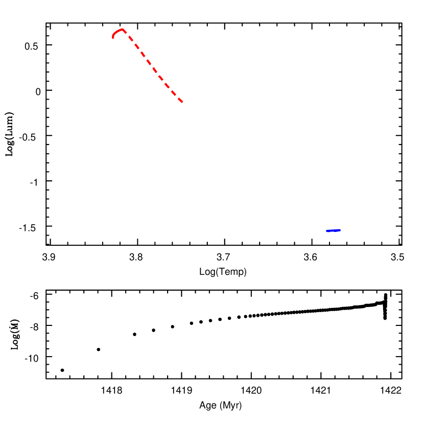
Figure 1: Case AD - Dynamic Contact. In the top panel of this figure, and in Figures  2 - 8, we show the evolution of both stars in an HR diagram. The track for $*1$ is always the initially more luminous, $*2$ the initially less luminous. Solid lines indicate periods where the binary is separated, dashed lines indicate periods where $*1$ is transferring mass to $*2$. We mark any transitions to the Hertzsprung Gap as H, and transitions to the Giant Branch as G. The bottom panel shows the mass transfer rate in logarithmic units of $\dot{M}/\rm$yr for the period in time during which mass transfer occurs. The initial parameters of this binary are $\log{M_{10}}=0.15$, $q_{0}=0.50$ and $\log P_{0}/P_{\rm ZAMS}=0.15$. The mass transfer rises rapidly to the dynamic timescale and the two stars come into contact.

  The calculation is terminated by (e) above, but seems likely to lead either to contact or to a common-envelope situation, and probably then to a complete merger of the two components. We illustrate the behaviour in the HRD and the mass transfer rate of case AD in Figure 1.

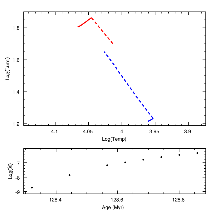
Figure 2: Case AR - Rapid Contact. The initial parameters of this binary are $\log{M_{10}}=0.45$, $q_{0}=0.15$ and $\log P_{0}/P_{\rm ZAMS}=0.10$. The mass transfer rate rises rapidly to the thermal timescale and the two stars come into contact with a final mass ratio $\log q=0.11$, still well above unity.

• AR – rapid evolution to contact: this occurs in binaries with moderate to large $q_{0}$. In these cases $*2$ expands so rapidly in response to the onset of $*1$’s thermal-timescale RLOF that it fills its own Roche lobe before much mass is transferred. We define the mass transfer rate to be thermal when the magnitude of the thermal luminosity, $\mid L_{\rm therm}\mid$, reaches 2% of the nuclear burning luminosity, $L_{\rm nuc}$. This probably leads to a contact binary of the W UMa type, although it can happen as easily for massive stars (provided $q_{0}$ is suitably large) as for the lower masses of typical W UMa systems. Case AR behavior is illustrated in Figure 2.

In some binary runs, these two cases are difficult to distinguish. While evolution of $*1$ will proceed through several timesteps of dynamic timescale mass transfer before being terminated by (e), the calculation of $*2$ is often unable to converge while gaining mass at this rate. The calculations of case AR and AD binaries at very large $q_{0}$, therefore, often terminate before contact is reached and we must guess the rate mass transfer achieves before contact occurs.

To do so we extrapolate the function $\log{\frac{R_{2}}{RL_{2}}(t)}$ to the time $t_{\rm contact}$ at which the radius of $*2$ has expanded to fill its RL and $\log{\frac{R_{2}}{RL_{2}}(t)}=0$. We then examine the mass loss history of $*1$ (whose calculation has proceeded further in time than that of $*2$) and determine whether the mass transfer rate reaches the thermal or dynamic timescale at $t\leq t_{\rm contact}$. Unfortunately, the function $\log{\frac{R_{2}}{RL_{2}}(t)}$ can be both non-linear and slightly noisy, and so $t_{\rm contact}$, along with the maximum mass transfer rate, can depend rather sensitively on the exact point in time at which $*2$ fails.

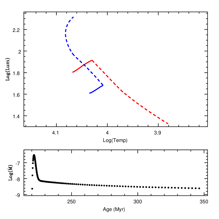
Figure 3: Case AS - Slow Contact. The initial parameters of this binary are $\log{M_{10}}=0.45$, $\log{q_{0}}=0.05$ and $\log P_{0}/P_{\rm ZAMS}=0.20$. Contact is avoided during the period of thermal scale mass transfer and a long period of nuclear timescale mass transfer follows. The run ends in contact with a final mass ratio, $\log{q}=-0.27$.

• AS – slow evolution to contact: this occurs in binaries with small $q_{0}$ and small $P_{0}$. These binaries experience a short burst of thermal timescale mass transfer, followed by a long phase of nuclear timescale mass transfer, during which much mass is exchanged. The two stars come into contact slowly, but reach contact before either star has left the MS. The large amount of mass transfer leads to a final mass ratio substantially below unity (typically $q\sim 0.4-0.6$), and with both stars substantially larger than their ZAMS radii. Case AS behavior is illustrated in Figure 3. We note that while $*2$ always remains near the main-sequence band, $*1$ evolves to substantially cooler temperatures. This is a common configuration in observed Algol systems.

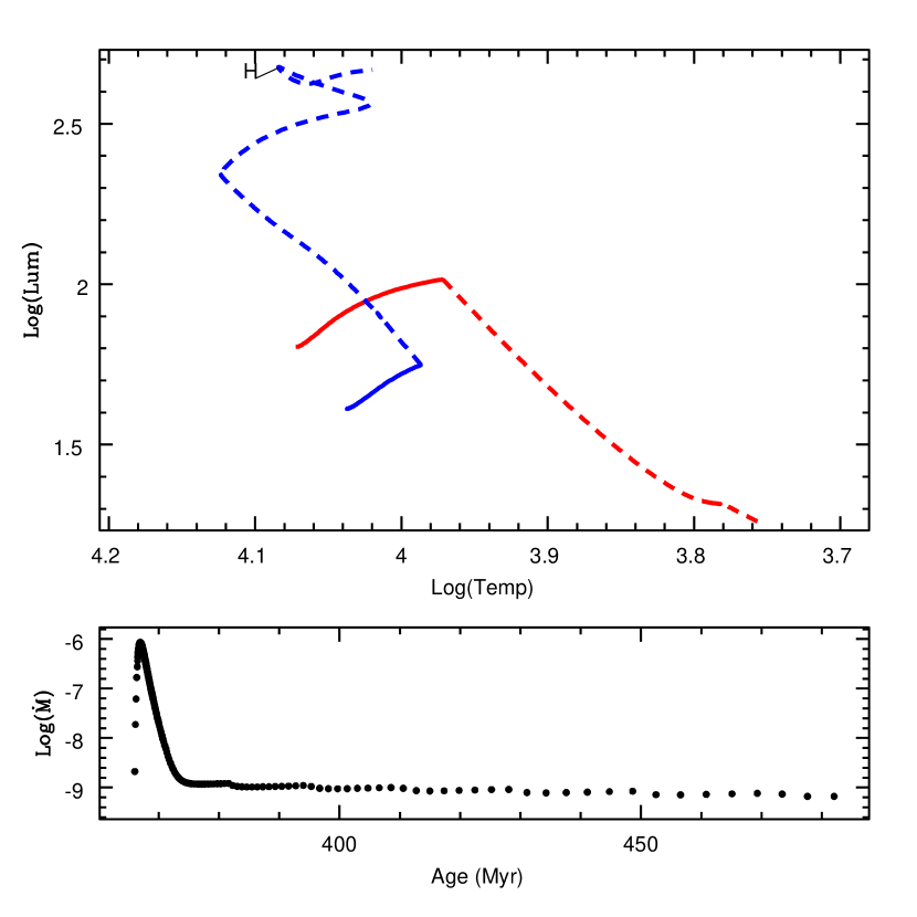
Figure 4: Case AE - Early Overtaking. The initial parameters of this binary are $\log{M_{10}}=0.45$, $\log{q_{0}}=0.05$ and $\log P_{0}/P_{\rm ZAMS}=0.45$. $*2$ gains so much mass that its evolution overtakes that of $*1$ and $*2$ reaches the HG first. The run ends in contact with a final mass ratio of $\log{q}=-0.23$.

• AE – early overtaking: this occurs in binaries with small $q_{0}$ and moderate $P_{0}$. It occurs only in binaries with initial masses $2M_{\odot}\lesssim M_{1}\lesssim 10M_{\odot}$. The mass transfer in this case is very similar to case AS. In case AE, however, $*2$ gains so much mass that its evolution is accelerated to the extent that $*2$ reaches the Hertzsprung Gap, HG, while $*1$ is still on the MS; the evolution of the initially less massive star, $*2$, has overtaken that of $*1$. We define the overtaking as early because it occurs with $*1$ still on the MS. Most case AE binaries reach contact shortly thereafter. However, in a few cases $*1$ shrinks very slightly inside its RL at the end of the calculation and the run ends with the RLOF of $*2$. In these cases, $*1$ has very nearly exhausted hydrogen and it is likely that it will soon swell once again to fill its RL and contact will again occur. Case AE behavior is illustrated in Figure 4.

In most cases where contact is avoided while $*1$ is on the MS, $*1$ loses so much mass that it eventually shrinks inside its RL leaving only a compact core. A period of separation ensues which may then be followed by further RLOF of $*1$ or $*2$. These are the cases AL, AB and AN, described in more detail below. However, in our lower mass binaries ($M_{10}\leq 1.6M_{\odot}$) we see a few cases where contact is avoided while $*1$ is on the MS, but reached later on.

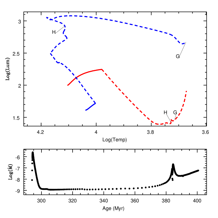
Figure 5: Case AG - Contact on Giant Branch. The initial parameters of this binary are $\log{M_{10}}=0.50$, $\log{q_{0}}=0.10$ and $\log P_{0}/P_{\rm ZAMS}=0.55$. The stars come into contact at a mass ratio of $\log{q}=-0.83$. There is a brief period of separation at $t\sim 384$ Myr with $*1$ in the HG.

• AG – contact on giant branch: this occurs for $M_{10}\lesssim 1.6M_{\odot}$, and $P_{0}$ larger then those of AS/AE, but smaller then AL/AN. Contact is avoided while $*1$ is on the MS, but occurs when $*1$ reaches the giant branch, GB. At time of contact $*2$ is in the HG or on the GB as well. A typical example of case AG is shown in Figure 5.

Cases AL, AN are distinguished by whether or not $*1$ supernovas before $*2$ reaches RLOF. In practice, we assume a supernovae explosion to be iminent when $*1$ begins burning carbon.

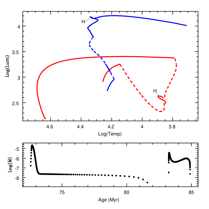
Figure 6: Case AL - Late Overtaking. The initial parameters of this binary are $\log{M_{10}}=0.75$, $\log{q_{0}}=0.05$ and $\log P_{0}/P_{\rm ZAMS}=0.60$. In this run $*1$ loses so much mass in two periods of mass transfer that it eventually shrinks inside its RL and becomes a low mass helium burning core, $\log{M_{1}}=-0.07$. The run ends as $*2$ crosses the HG and fills its RL at a very low mass ratio, $\log q=-1.07$. The brief period of separation between the two bursts of mass transfer is a feature common to all of our higher mass case AL/AN binaries. This feature occurs as $*1$ exhausts hydrogen in the core, convection in the core shuts off and $*1$ shrinks slightly inside its RL. At this point $*1$ behaves as a “normal” massive terminal MS star, executing the classic hook at the end of the MS. When hydrogen is completely exhausted in the core and hydrogen shell burning begins $*1$ starts to cross the HG. During this rapid phase of envelope expansion, $*1$ quickly fills its RL again and mass transfer begins again.

• AL – late overtaking: this occurs in binaries with $M_{10}\lesssim 13M_{\odot}$ and moderate to large $P_{0}$. In these binaries, $*2$ reaches RLOF before $*1$ begins burning carbon. In many of the lower-mass AL cases, $*1$ has become a low mass remnant (WD or NS) which will never supernovae unless the (uncomputed) reverse mass transfer results in significant mass gain for $*1$. The evolution of $*2$ has overtaken the evolution of $*1$ in the sense that the initially more massive star is now shrunk inside its RL while the initially less massive star is undergoing RLOF. The overtaking is late because it occurs with $*1$ past the MS. Case AL behavior is illustrated in Figure 6.

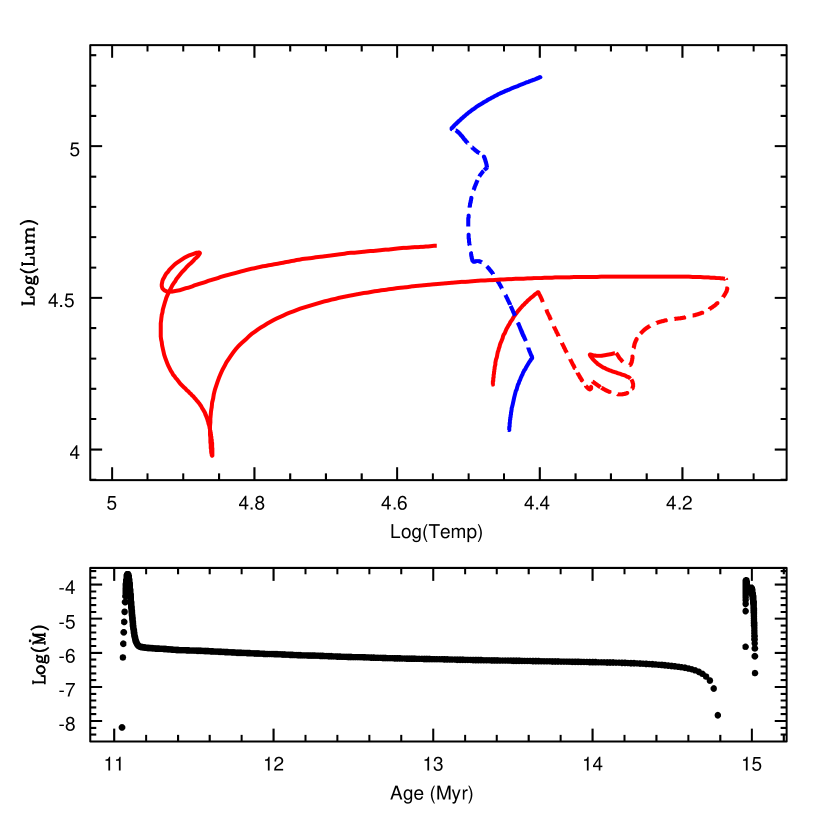
Figure 8: Case AN - No Overtaking. The initial parameters of this binary are $\log{M_{10}}=1.15$, $\log{q_{0}}=0.05$ and $\log P_{0}/P_{\rm ZAMS}=0.45$. After two periods of mass transfer, $*1$ becomes a helium star of mass $\log{M_{1}}=0.48$. As $*2$ evolves towards the terminal MS, $*1$ ignites carbon in the core. The ignition of carbon suggests an imminent supernovae explosion, and we conclude that $*1$ will supernovae before $*2$ fills its RL.

• AN – no overtaking: this occurs in higher mass binaries with moderate to large $P_{0}$. In these binaries $*1$ reaches carbon burning, indicating an imminent supernova, before $*2$ has reached RLOF. Case AN behavior is illustrated in Figure 8.

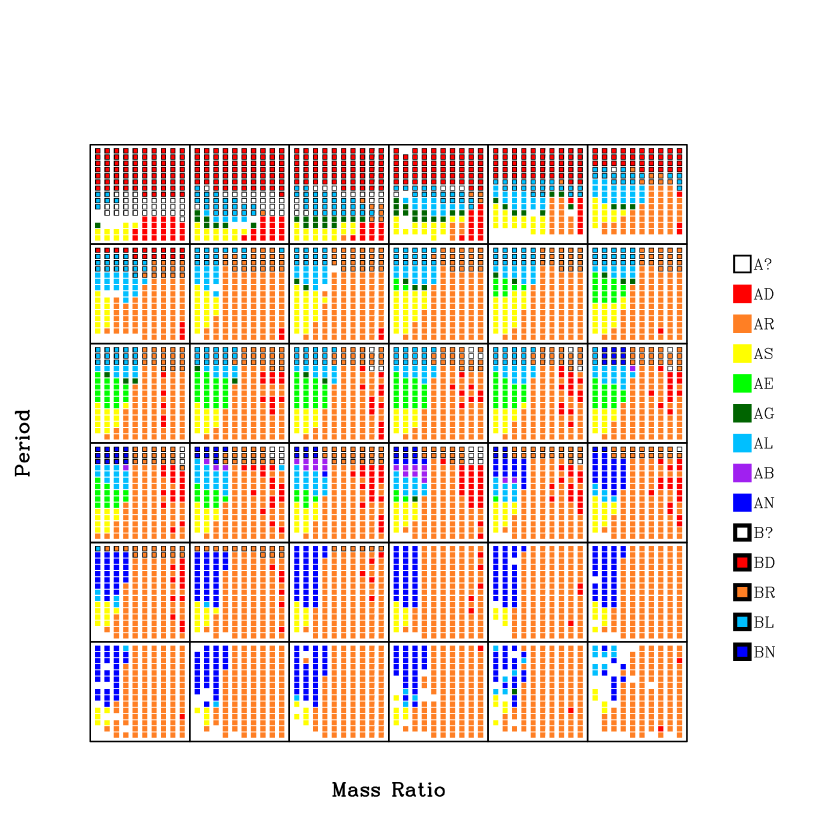
Figure 9: The classification of each of our individual binary runs into cases AD, AR, AS, AE, AG, AL, AB, AN, BD, BR, BL, and BN, as described in §3. Each square represents a slice through the data cube at constant $M_{10}$. The upper left hand block is a slice at $\log{M_{10}}=-0.05$. The squares increase in the order one reads the page of a book, increasing in units of $0.05$ and ending in the bottom right hand corner with $\log{M_{10}}=1.70$. We do not show our results for $\log{M_{10}}=-0.10$ as very few of these binaries reached RLOF at an age younger then 20 Gyr. Within each square the x-axis represents increasing mass ratio in logarithmic units of $0.05$ from $\log{q}=0.05$ to $0.50$. The y-axis represents increasing period in units of $0.05$ from $\log P_{0}/P_{\rm ZAMS}=0.05$ to $0.75$, where $P_{\rm ZAMS}$ is the critical period at which RLOF would occur on the ZAMS. The color of each dot represents the classification of the binary run according to the legend to the right of the plot. A white dot represents a Case A binary for which we could not determine a sub-class, a white dot outlined in black indicates a Case B binary for which we could not determine a sub-class.

As discussed in §2 the evolution of our most massive stars, $M_{10}\gtrsim 25M_{\odot}$ often breaks down. This leads us again to the situation where we must make a best guess as to what happens after the run stops. To distinguish case AL from AN we must determine whether $*2$ reaches RLOF before $*1$ ignites carbon. This procedure is somewhat uncertain and leads to the great majority of our unclassified runs at very high mass. We also suspect that several of the highest mass runs, $M_{10}\gtrsim 40M_{\odot}$, which were classified as AL are uncertain, and may more probably be Case AN. (See Figure 9.)

We note that the definitions of case AL and AN given here do not correspond exactly to those of Eggleton (2000). In this previous work, case AN also included those binaries where $*1$ had become a WD or NS before $*2$ filled its RL. In this work, those binaries are included in case AL.

Pols (1994) noted that occasionally, in what we call case AL here, $*2$ could get to carbon ignition before $*1$, and thus be the first component to explode as a supernova. Pols (1994) modeled, in a simple way, the effect of the presumed common-envelope phase in ejecting $*2$’s envelope, and then continued the evolution of the core. Although it would always have started He burning later than $*1$, it might be sufficiently more massive to overtake and ignite carbon first. However, in our work we did not attempt to model the common-envelope phase at all, and so we cannot be definitive about this possibility.

In addition, we include one more class: the classic Case AB. In our context this is a subclass of case AL, where $*1$, after becoming a compact helium core with a mass of $\sim 1-2M_{\odot}$, expands again and experiences a further period of RLOF.

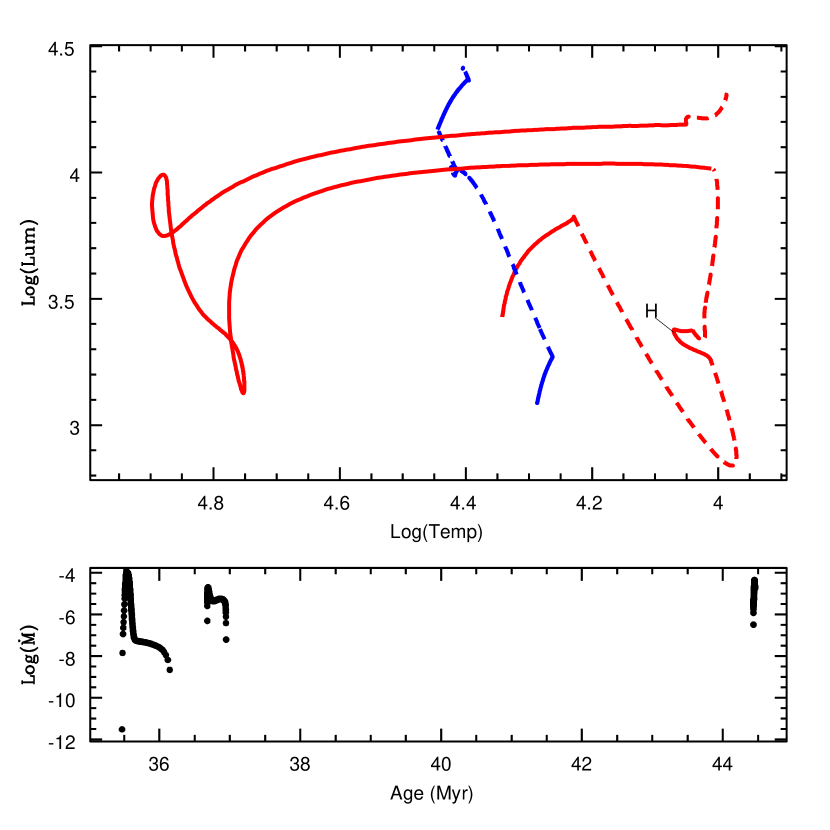
Figure 7: Case AB - (Sub-type of AL). The initial parameters of this binary are $\log{M_{10}}=0.90$, $\log{q_{0}}=0.10$ and $\log P_{0}/P_{\rm ZAMS}=0.65$. After igniting helium towards the end of the second burst of mass transfer, $*1$ shrinks inside its RL for awhile, but eventually re-expands and undergoes a third period of mass transfer.

• AB - this occurs in binaries with $6M_{\odot}\lesssim M_{10}\lesssim 11M_{\odot}$, at small mass ratios and in a narrow range of periods between cases AL and AN. During the second burst of mass transfer, $*1$ ignites helium. It shrinks inside its RL for awhile, becoming a compact helium star. It then expands again and experiences a third period of mass transfer. Although these binaries often fail to converge at some point during this third period of mass transfer, we suspect that it is followed by a period of separation and then reverse mass transfer, making this a subclass of AL rather then AN. An example of case AB evolution is shown in Figure 7.

In Table 1 we summarize the seven major subcases (excluding case AB), providing the defining equations as well the evolutionary state and geometrical configuration of the binary components at the end of the calculation. In this table we denote the main sequence as M, the Hertzsprung Gap as H, the giant branch as G, and low and high mass remnants as R and C, respectively. In addition, we define the time of first RLOF, $t_{\rm RLOF}$, the approximate MS lifetime of a single star, $t_{\rm MS}$, the time at which the star enters the Hertzprung Gap, $t_{\rm H}$ and the time at which carbon is ignited $t_{\rm Cburn}$. We emphasize that we execute the classification of each binary in our library automatically, and while the various clauses we define work for the great majority of systems, we inevitably make a few misclassifications.

As mentioned above, figures 1 - 8 illustrate the behaviour in the HRD of the subtypes of Case A. We also show the mass transfer rate for times when $\dot{M}>0$. Figure 9 shows which elements of our data cube reached which outcome. Some of the systems of longer $P_{0}$ are Case B rather than Case A. These are usually analogous to either AD, AR, AL or AN. Case BD is effectively the classical Late Case B, where $*1$ reaches the giant branch and acquires a deep convective envelope before RLOF begins; however it can also be an extreme initial mass ratio rather than a convective envelope which triggers dynamic mass transfer. Case B systems, or at least those which we have computed here, normally have fewer options than Case A because it is difficult for $*2$ to catch up with $*1$ when $*1$ has already reached the terminal main sequence before RLOF. However, as emphasised by De Greve & Packet (1990), it is possible for early Case B systems to show what we call here Case BL for late overtaking, with $*2$ evolving to fill its own Roche lobe while $*1$ has shrunk inside its own. This kind of behaviour is particularly prevalent in the mass range $M_{10}\lesssim 8M_{\odot}$.

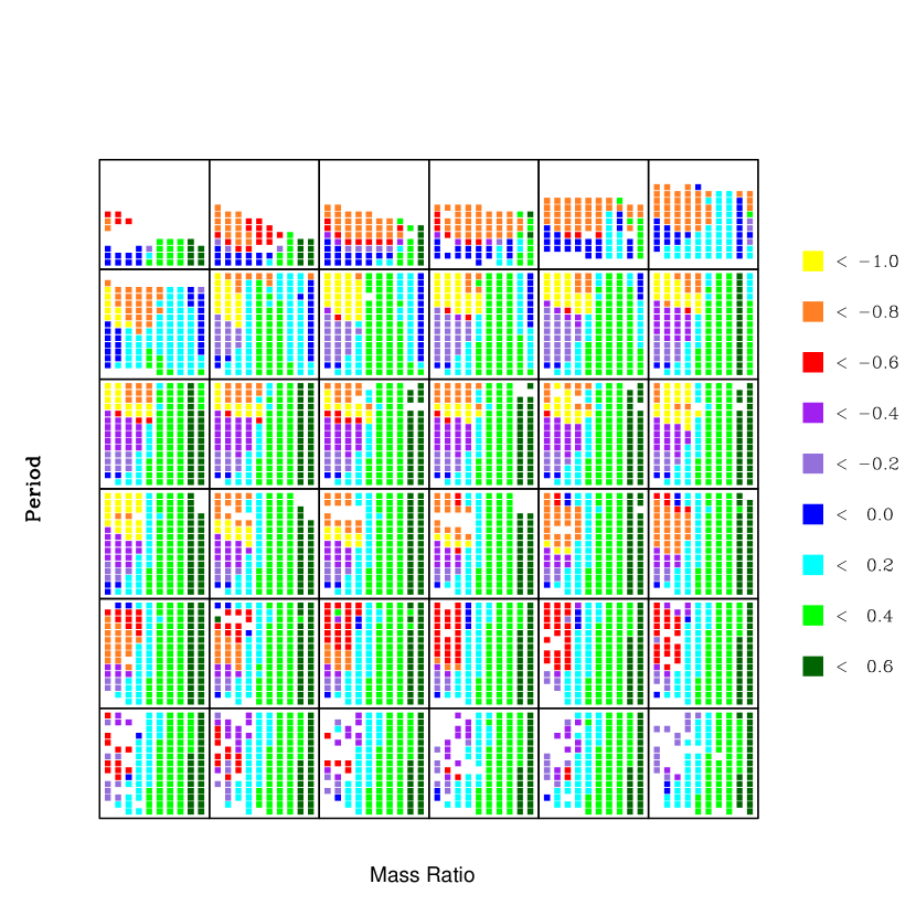
Figure 10: The final mass ratio of each binary system. The ordinates are defined as in Figure 9. We define the final state to be the point where either a) contact is reached or seems imminent, b) reverse mass transfer begins, c) $*1$ has ignited carbon or d) the binary is in a detached phase and reverse mass transfer is imininent. Binaries for which the final state could not be determined appear as white squares. Higher mass white squares are generally due to binaries which break down during thermal timescale mass transfer. The color-coded final mass ratios are in logarithmic units. The legend is to be interpreted as follows: binaries with $\log q<-1.0$ are shown as yellow squares, those with $-1.0\leq\log q<-0.8$ as orange squares, and so forth.

In Figures 10 and 11 we show, also in colour-coded form, the following two properties of systems in our data cube: (i) the final mass ratio of each system and (ii) the fraction of time spent as a semidetached system. We define the state of the binary to be final when a) contact is reached, b) reverse mass transfer begins, c) $*1$ has ignited carbon, or d) the binary is detached and we believe reverse mass transfer to be imminent (ie. the function $\log{\frac{R_{2}}{RL_{2}}(t)}$ will soon reach zero). The time spent as a semi-detached system has implications for the frequency of Algols in the field. We find that for a given primary mass the longest-lived Algols originate from systems where mass transfer begins near the transition to the HG (Late Case A to Early Case B or cases AL, AN, BL, BN) and with small to moderate initial mass ratios.

4 Comparison with Observed Systems

Many observed binaries are semidetached (Algols), and one might hope that they could be matched by some of the above theoretical models during their stage of RLOF. However it has been clear for some time (Refsdal, Roth & Weigert 1974) that at least some systems (specifically, AS Eri) have such low angular momentum that they could hardly have started as detached systems of two zero-age main sequence stars of comparable mass. Furthermore there are some Algols of such low total mass (e.g. R CMa) that they also could hardly have started in such a configuration.

In an important paper, Maxted & Hilditch (1996) identified 9 Algol systems for which they thought the observational data was of an unusually high quality. They compared these with models computed by De Greve (1993). The comparison was not at all satisfactory, the theoretical models having luminosities at least 20 times greater than the observed models. They also had substantially longer periods. These discrepancies appear to be due to the following two features:

1. the theoretical models were all Case B

2. they were non-conservative, the assumption being made that 50% of the mass lost by $*1$ escaped to infinity, and 50% was accreted by $*2$. The escaping mass was assumed to remove the same specific angular momentum as resided in the orbit of $*1$.

We feel that although the kind of non-conservation modeled by De Greve (1993) may perhaps be appropriate for massive stars (O, and even early B), where radiation pressure may be an important agent in mass loss, it is not appropriate for mid-main sequence stars where, at least in single stars, very little mass loss is normally observed. At the other end of the main sequence, stellar winds are rather commonly observed, particularly in rapidly rotating G/K/M dwarfs (and even more so in giants). These winds probably do not carry off much mass (although see later), but they may be rich in angular momentum because of magnetic linkage to the parent star. We therefore think that conservative models may be reasonable for systems which are in the middle of the main sequence initially (say B1 to G0), and where the loser has not yet evolved to the red-giant region at spectra type $\sim$G or later. Following Popper (1980) we refer to these systems as ‘hot Algols’. Unfortunately rather few of the Maxted & Hilditch (1996) selection qualify as hot Algols in this sense, although two (U CrB and AF Gem) are on the border, with the cooler component having spectral type $\sim$G0. We have therefore included a few more from the literature. Our selection of hot Algols is listed in Table 2, with references.

The observed parameters which we attempt to fit with our theoretical models are the six independent quantities $\log P$, $\log M_{1}$, $\log q$, $\log R_{2}$, $\log T_{1}$ and $\log T_{2}$. $R_{1}$ is not independent of these, since it is obtained from the assumption that $*1$ fills its Roche lobe, whose radius is determined by the first 3 parameters. $L_{1}$ and $L_{2}$ are similarly not independent of these 6 parameters. Our theoretical models have four independent parameters, $\log P_{0}$, $\log M_{10}$, $\log q_{0}$ and age.

For each system in Tables 2 and 3 we give three rows. The first gives the observational data from the literature, and the next the theoretical values from our data cube which minimize $\chi^{2}$. The second row also includes the best-fit age, in units of Myr. The third row gives the zero-age values for the system which we infer from our best fit. We use mass-ratio $q$ because this is usually obtained more directly from the observational data, whether spectroscopic or photometric, than either $M_{1}$ or $M_{2}$. We list observational errors (when available) in the first row for all quantities, but we list total errors (described below) in the second row only for those quantities that we actually fit.

In fitting observed stars to theoretical models, a $\chi^{2}$ test seems appropriate. However, we have to modify the standard test in order to incorporate the fact that our theoretical models have an intrinsic ‘graininess’ because they have not been computed for a continuous range of input parameters, but only at the grid-points in our data cube. We therefore use a total error, $\sigma$, which is the sum in quadrature of the observational error, $\sigma_{\rm obs}$, and a ‘theoretical error’, $\sigma_{\rm th}$, representing the intrinsic graininess. For $\log P,~{}\log M_{1}$ and $\log q$ we take $\sigma_{\rm th}=0.05$, the initial spacing of our grid. For $\log R$ and $\log T$ we take the graininess to be the difference in these parameters between adjacent ZAMS models from the grid, centered on the mass of the observed binary. For example, for an observed star of mass $\log M=1.02$ we take the theoretical error in the radius to be

$$\sigma_{\rm th,R}(\log M=1.02)=R_{\rm ZAMS}(\log M=1.05)-R_{\rm ZAMS}(\log M=1.00)~{}.$$ (9)

We can then look in our data cube for the minimum value of

$$\chi^{2}=\sum{\frac{({\rm obs-th})^{2}}{\sigma_{\rm obs}^{2}+\sigma_{\rm th}^{2}}}~{}.$$ (10)

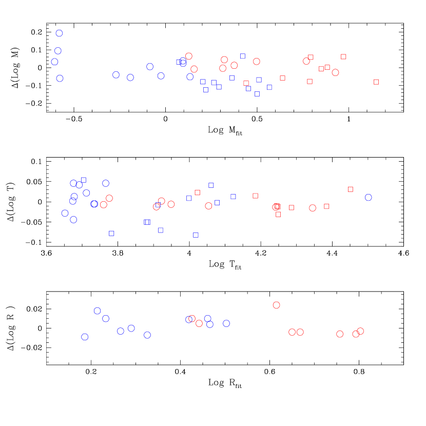
Figure 12: The residuals of observed binary fits. The hot Algols of Table 2 are shown in red, the cool Algols of Table 3 are shown in blue. The residuals of $*1$ are shown as circles, the residuals of $*2$ as squares. The residuals are defined in the sense $\Delta=\rm{fit}-\rm{obs}$ .

We find that the best fit point picked by minimizing this $\chi^{2}$ is insensitive to the exact definition of $\sigma_{\rm th}$. However, the magnitude of $\chi^{2}_{\rm min}$ depends directly on $\sigma$, so we have attempted a reasonable definition. In Figure 12 we present the residuals to the fit for all Algols from both Tables 2 and 3.

The hot Algols of Table 2 have a mean $\chi^{2}$ of $\sim 3$. Since there are 2 degrees of freedom (6 observed parameters less 4 theoretical parameters), this value is rather more, but not enormously more, than is expected for a normal distribution of errors. The number of systems which we use is too small to provide a really convincing confirmation or refutation. The worst case, AF Gem, is very close to the lower temperature limit, where we suppose a priori that conservation might break down. If we reject AF Gem, we have a mean $\chi^{2}$ of just 2.

After AF Gem, the next worse cases are DM Per and $\lambda$ Tau. Interestingly, both of these systems possess a close third body – extraordinarily close in the case of $\lambda$ Tau. The latter system can be seen to be problematic even without a detailed attempt at fitting. The angular momentum of this system is seen to be quite low compared with a system of comparable-mass stars at the same total mass, so that something like Case AS is to be expected. But Case AS normally evolves into contact at a mass ratio which is moderately small, roughly $\gtrsim 0.4$ (Figure 10), whereas $\lambda$ Tau has quite a small present mass ratio of $0.27$. This suggests that $\lambda$ Tau has lost some angular momentum, necessarily during its slow, nuclear-timescale, RLOF rather than the comparable interval of detached evolution before RLOF. DM Per’s problem is similar, though not so obvious without a detailed attempt at fitting.

But for $\lambda$ Tau and DM Per, unlike most other hot Algols, there does in fact exist a mechanism that should do just that. The third star in the $\lambda$ Tau system (Fekel & Tomkin, 1982) is in such a close orbit ($33$d) that it must influence the orbit of the eclipsing pair to a small but significant extent, making its eccentricity fluctuate by $\sim 0.7\%$ on a timescale of days (Kiseleva, Eggleton & Mikkola, 1998). Tidal friction will tend to oppose this, but can only do so by draining energy and angular momentum from the short-period orbit. Conservation laws require the angular momentum lost by the inner orbit to go to the outer orbit, but the energy loss leads to a net secular evolution, the inner orbit shrinking while the outer widens. This process was probably negligible in the pre-RLOF state because the orbit would have been substantially smaller than at present, at least if $q_{0}$ were not unusually large. But it can now be significant as the stars are larger and the inner orbit wider. Tidal friction should be capable of setting up a transient equilibrium between nuclear evolution, leading to expansion of the inner orbit, and tidal friction, leading to contraction (Kiseleva, Eggleton & Mikkola, 1998).

DM Per also has a third body in orbit. The outer orbit is longer ($\sim 100$d) while the inner orbit is shorter, and so the process might be thought less likely to be significant. But on the other hand the third body is relatively much more massive, which may compensate to some extent.

When we turn to a selection of cooler Algols (Table 3) we find significantly larger $\chi^{2}$ for many systems. This, we believe, is consistent with the view that they are less conservative, certainly of angular momentum (which is fairly readily removed by magnetic braking on something like a nuclear timescale), and perhaps also of mass. We do not normally think of stellar winds from cool dwarfs and subgiants as being strong enough to remove significant mass, and yet certain active (RS CVn) binaries show evidence to the contrary. Both Z Her (Popper, 1988) and to a lesser extent RW UMa (Popper, 1980; Scaltriti et al., 1993) exhibit the phenomenon that the cooler, presumably more evolved, subgiant is the less massive star, despite the fact that it does not fill its Roche lobe. This suggests that mass loss by wind from the cooler star is already on the nuclear timescale of the star.

V1379 Aql (Jeffery & Simon, 1997) is an example of a ‘post-Algol’ binary: the low-mass SDB component is presumably the remains of $*1$ after it has retreated within its Roche lobe, and $*2$ has already evolved to the giant branch. We include it in our list of cool Algols as we believe the components to have been relatively cool during its Algol phase. The cool ZAMS temperatures which we derive support this assumption. Even without detailed fitting, it is clear that the system is problematic. For a period as short as 21d the SDB mass is rather large – such a core would seem to imply a period of 50 – 100d. More intriguingly, the orbit is very significantly eccentric: $e=0.09\pm 0.01$. Several radio pulsars with WD companions are known with comparable period and with highly circular orbits – e.g. 1855+09 (Ryba & Taylor, 1991) – as expected following stable RLOF from a low-mass giant. Probably the least far-fetched explanation of the eccentricity in V1379 Aql is the presence of a third body in a substantially inclined orbit; and this might also explain some loss of angular momentum.

5 Conclusions

Case A RLOF, even when restricted to the classical ‘conservative’ model, shows a rich variety of behaviour, which we feel is often not emphasised enough. We identify 9 sub-classes, depending partly on whether the system evolves into contact (in 5 different ways) or reaches reverse RLOF (in 4 different ways). Further subdivision depends on the evolutionary states reached when contact or reverse RLOF occurs. We can expect even more subclasses when non-conservative processes are modeled, as will certainly be necessary for extremes of high-temperature and low-temperature systems.

For all but one of our selection of observed hot Algols we find an acceptable $\chi^{2}$ when fitting the observed parameters to our library of conservative Case A binary tracks. It is encouraging to note that the worst outlier (AF Gem) lies near the lower boundary of the temperature range in which we expect the conservative assumption to hold. The next largest $\chi^{2}$’s come from two binaries with known third bodies, which may act to remove angular momentum from the inner orbit.

Our selection of cool Algols shows significantly worse agreement between the observed systems and the conservative theoretical tracks, suggesting the need for more free parameters in the modelling, such as mass and angular momentum loss.

This data set of conservative Case A tracks has uses beyond an indiviual comparison of observed systems. With an estimate of the initial mass function and period distribution of binaries, it may be useful for population synthesis studies or for creating close binary-inclusive isochrones for stellar population studies. We hope to make these tracks available in early 2001 on the Institute of Geophysics and Planetary Physics web site http://www.llnl.gov/urp/IGPP.

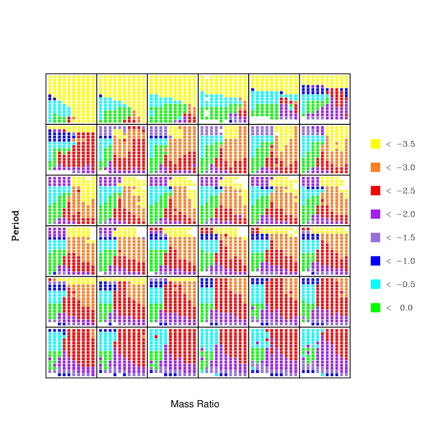
Figure 11: The fraction of a given binary’s lifetime time spent transferring mass from $*1$ to $*2$, $f_{\rm RLOF}$. The ordinates are defined as in Figure 9. The blank squares are those binaries which failed to converge for more then a few timesteps. The color-coded fractions are in logarithmic units. The legend is to be interpreted as follows: binaries with $\log f_{\rm RLOF}<-3.5$ are shown as yellow squares, those with $-3.5\leq f_{\rm RLOF}<-3.0$ as orange squares, and so forth.

Table 1: Summary of Binary Classification Scheme

Case	Defining Equations	End State $*1$	End State $*2$	End Geometry
AD	$\dot{M}>M/t_{\rm dyn}$	M	M	Contact
AR	$\dot{M}>M/t_{\rm KH}$, $t_{\rm contact}-t_{\rm RLOF}(*1)<0.10\times t_{\rm MS}(*1)$	M	M	Contact
AS	$t_{\rm contact}-t_{\rm RLOF}(*1)>0.10\times t_{MS}(*1)$	M	M	Contact
AE	$t_{\rm H}(*2)<t_{\rm H}(*1)$	M	H	Contact
AG	$t_{\rm H}(*1)<t_{\rm H}(*2)$	G	H,G	Contact
AL	$t_{\rm RLOF}(*2)<t_{\rm Cburn}(*1)$	R,C	H,G	RLOF $*2$
AN	$t_{\rm Cburn}(*1)<t_{\rm RLOF}(*2)$	SNe	M,H,G	Detached

Table 2: Hot Algols: observed, best fit and ZAMS parameters

	log	log		log		log		log		log		log		log		log
Star	$P$	$M_{1}$	$\sigma_{M_{1}}$	$q$	$\sigma_{q}$	$T_{1}$	$\sigma_{T_{1}}$	$T_{2}$	$\sigma_{T_{2}}$	$R_{1}$	$\sigma_{R_{1}}$	$R_{2}$	$\sigma_{R_{2}}$	$L_{1}$	$\sigma_{L_{1}}$	$L_{2}$	$\sigma_{L_{2}}$	Age	$\chi^{2}$
TT Aur9	0.124	0.732	0.023	-0.175	0.010	4.255	0.020	4.395	0.020	0.623	0.010	0.591	0.011	3.210	0.030	3.710	0.030	$\cdots$	$\cdots$
$\cdots$	0.149	0.769	0.055	-0.201	0.051	4.242	0.035	4.384	0.033	0.650	$\cdots$	0.615	0.031	3.220	$\cdots$	3.720	$\cdots$	16	1.775
$\cdots$	0.119	0.950	$\cdots$	0.150	$\cdots$	4.369	$\cdots$	4.287	$\cdots$	0.581	$\cdots$	0.493	$\cdots$	3.593	$\cdots$	3.088	$\cdots$	$\cdots$	$\cdots$
U CrB4	0.538	0.164	0.023	-0.420	0.022	3.767	0.015	4.170	0.009	0.694	0.008	0.436	0.011	1.430	0.060	2.510	0.130	$\cdots$	$\cdots$
$\cdots$	0.547	0.158	0.055	-0.481	0.055	3.761	0.049	4.187	0.031	0.703	$\cdots$	0.433	0.032	1.403	$\cdots$	2.567	$\cdots$	218	1.604
$\cdots$	0.235	0.550	$\cdots$	0.200	$\cdots$	4.137	$\cdots$	4.003	$\cdots$	0.341	$\cdots$	0.227	$\cdots$	2.185	$\cdots$	1.417	$\cdots$	$\cdots$	$\cdots$
AF Gem7	0.095	0.063	0.015	-0.466	0.010	3.767	0.010	4.000	0.020	0.365	0.007	0.417	0.010	0.750	0.030	1.780	0.090	$\cdots$	$\cdots$
$\cdots$	0.124	0.127	0.052	-0.313	0.051	3.776	0.027	4.023	0.037	0.414	$\cdots$	0.426	0.032	0.883	$\cdots$	1.897	$\cdots$	635	11.394
$\cdots$	0.026	0.400	$\cdots$	0.200	$\cdots$	4.038	$\cdots$	3.878	$\cdots$	0.254	$\cdots$	0.169	$\cdots$	1.612	$\cdots$	0.803	$\cdots$	$\cdots$	$\cdots$
u Her5	0.312	0.462	0.029	-0.409	0.022	4.064	0.020	4.300	0.020	0.643	0.029	0.763	0.022	2.490	0.060	3.680	0.050	$\cdots$	$\cdots$
$\cdots$	0.330	0.497	0.058	-0.386	0.055	4.054	0.039	4.286	0.033	0.673	$\cdots$	0.757	0.037	2.516	$\cdots$	3.612	$\cdots$	64	0.949
$\cdots$	0.120	0.800	$\cdots$	0.150	$\cdots$	4.287	$\cdots$	4.200	$\cdots$	0.493	$\cdots$	0.402	$\cdots$	3.088	$\cdots$	2.554	$\cdots$	$\cdots$	$\cdots$
DM Per6	0.436	0.316	0.012	-0.547	0.011	3.920	0.010	4.260	0.020	0.677	0.008	0.653	0.009	2.000	0.060	3.280	0.100	$\cdots$	$\cdots$
$\cdots$	0.488	0.313	0.052	-0.474	0.051	3.908	0.039	4.248	0.034	0.715	$\cdots$	0.650	0.031	2.016	$\cdots$	3.243	$\cdots$	114	3.379
$\cdots$	0.187	0.700	$\cdots$	0.200	$\cdots$	4.229	$\cdots$	4.106	$\cdots$	0.432	$\cdots$	0.311	$\cdots$	2.735	$\cdots$	1.997	$\cdots$	$\cdots$	$\cdots$
V Pup8	0.163	0.954	0.046	-0.277	0.068	4.360	0.060	4.420	0.040	0.724	0.024	0.799	0.020	3.850	0.250	4.200	0.160	$\cdots$	$\cdots$
$\cdots$	0.185	0.927	0.068	-0.223	0.085	4.345	0.065	4.451	0.045	0.724	$\cdots$	0.793	0.034	3.784	$\cdots$	4.344	$\cdots$	10	1.311
$\cdots$	0.117	1.100	$\cdots$	0.100	$\cdots$	4.444	$\cdots$	4.395	$\cdots$	0.668	$\cdots$	0.610	$\cdots$	4.065	$\cdots$	3.755	$\cdots$	$\cdots$	$\cdots$
$\lambda$Tau2,3	0.597	0.276	0.009	-0.578	0.007	3.920	0.030	4.280	0.040	0.724	0.016	0.806	0.007	2.110	$\cdots$	3.690	$\cdots$	$\cdots$	$\cdots$
$\cdots$	0.641	0.321	0.051	-0.529	0.050	3.922	0.048	4.249	0.048	0.819	$\cdots$	0.803	0.030	2.281	$\cdots$	3.557	$\cdots$	99	2.918
$\cdots$	0.254	0.750	$\cdots$	0.200	$\cdots$	4.259	$\cdots$	4.138	$\cdots$	0.463	$\cdots$	0.341	$\cdots$	2.913	$\cdots$	2.185	$\cdots$	$\cdots$	$\cdots$
Z Vul1,8	0.391	0.362	0.018	-0.367	0.039	3.955	0.020	4.255	0.040	0.653	0.019	0.672	0.018	2.070	0.060	3.300	0.160	$\cdots$	$\cdots$
$\cdots$	0.387	0.375	0.053	-0.417	0.063	3.949	0.041	4.245	0.049	0.670	$\cdots$	0.668	0.035	2.088	$\cdots$	3.268	$\cdots$	107	0.776
$\cdots$	0.137	0.700	$\cdots$	0.150	$\cdots$	4.229	$\cdots$	4.138	$\cdots$	0.432	$\cdots$	0.341	$\cdots$	2.735	$\cdots$	2.185	$\cdots$	$\cdots$	$\cdots$

References. — (1) Cester et al. (1977); (2) Fekel & Tomkin (1982); (3) Giuricin, Mardirossian & Mezzetti (1983) (4) Heintze & van Gent (1988); (5) Hilditch (1984); (6) Hilditch, Hill & Khalesseh (1992) (7) Maxted & Hilditch (1995); (8) Popper (1980); (9) Popper & Hill (1991);

Table 3: Cool Algols: observed, best fit and ZAMS parameters

	log	log		log		log		log		log		log		log		log
Star	$P$	$M_{1}$	$\sigma_{M_{1}}$	$q$	$\sigma_{q}$	$T_{1}$	$\sigma_{T_{1}}$	$T_{2}$	$\sigma_{T_{2}}$	$R_{1}$	$\sigma_{R_{1}}$	$R_{2}$	$\sigma_{R_{2}}$	$L_{1}$	$\sigma_{L_{1}}$	$L_{2}$	$\sigma_{L_{2}}$	Age	$\chi^{2}$
S Cnc15,9	0.977	-0.638	0.036	-1.045	0.001	3.665	0.010	3.990	0.010	0.720	0.004	0.332	0.004	1.050	0.050	1.580	0.045	$\cdots$	$\cdots$
$\cdots$	1.033	-0.605	0.062	-0.897	0.050	3.678	0.039	3.920	0.036	0.773	$\cdots$	0.326	0.028	1.210	$\cdots$	1.283	$\cdots$	4182	14.447
$\cdots$	-0.055	0.150	$\cdots$	0.250	$\cdots$	3.832	$\cdots$	3.680	$\cdots$	0.148	$\cdots$	-0.144	$\cdots$	0.580	$\cdots$	-0.614	$\cdots$	$\cdots$	$\cdots$
R CMa12,13	0.055	-0.775	0.049	-0.801	0.029	3.630	0.030	3.860	0.030	0.025	0.028	0.196	0.027	-0.410	0.160	0.760	0.180	$\cdots$	$\cdots$
$\cdots$	0.152	-0.580	0.070	-0.653	0.058	3.676	0.048	3.782	0.039	0.192	$\cdots$	0.214	0.077	0.041	$\cdots$	0.508	$\cdots$	19470	22.871
$\cdots$	-0.319	0.000	$\cdots$	0.350	$\cdots$	3.751	$\cdots$	3.569	$\cdots$	-0.050	$\cdots$	-0.386	$\cdots$	-0.143	$\cdots$	-1.544	$\cdots$	$\cdots$	$\cdots$
RZ Cas5	0.077	-0.137	0.012	-0.480	0.010	3.672	0.020	3.934	0.005	0.288	0.007	0.223	0.008	0.160	0.080	1.120	0.020	$\cdots$	$\cdots$
$\cdots$	0.109	-0.192	0.051	-0.412	0.051	3.674	0.043	3.884	0.036	0.296	$\cdots$	0.233	0.028	0.239	$\cdots$	0.954	$\cdots$	3971	5.382
$\cdots$	-0.105	0.150	$\cdots$	0.200	$\cdots$	3.832	$\cdots$	3.718	$\cdots$	0.148	$\cdots$	-0.102	$\cdots$	0.580	$\cdots$	-0.379	$\cdots$	$\cdots$	$\cdots$
TV Cas4	0.258	0.185	0.014	-0.393	0.008	3.720	0.040	4.020	0.020	0.517	0.007	0.498	0.008	0.860	0.170	2.030	0.090	$\cdots$	$\cdots$
$\cdots$	0.265	0.134	0.052	-0.376	0.051	3.766	0.060	4.061	0.037	0.509	$\cdots$	0.503	0.032	1.033	$\cdots$	2.202	$\cdots$	502	2.925
$\cdots$	0.097	0.450	$\cdots$	0.200	$\cdots$	4.072	$\cdots$	3.924	$\cdots$	0.282	$\cdots$	0.183	$\cdots$	1.806	$\cdots$	1.014	$\cdots$	$\cdots$	$\cdots$
AS Eri1,10	0.426	-0.682	0.018	-0.968	0.012	3.720	0.030	3.930	0.030	0.340	0.023	0.196	0.016	0.470	$\cdots$	1.060	$\cdots$	$\cdots$	$\cdots$
$\cdots$	0.542	-0.587	0.053	-0.791	0.051	3.676	0.048	3.880	0.048	0.451	$\cdots$	0.186	0.029	0.558	$\cdots$	0.848	$\cdots$	3474	22.549
$\cdots$	-0.005	0.150	$\cdots$	0.500	$\cdots$	3.832	$\cdots$	3.569	$\cdots$	0.148	$\cdots$	-0.386	$\cdots$	0.580	$\cdots$	-1.544	$\cdots$	$\cdots$	$\cdots$
TT Hya9,15	0.842	-0.229	0.132	-0.646	0.002	3.680	0.010	3.990	0.010	0.769	0.029	0.290	0.028	1.200	0.080	1.500	0.070	$\cdots$	$\cdots$
$\cdots$	0.846	-0.270	0.141	-0.633	0.050	3.652	0.039	3.999	0.036	0.759	$\cdots$	0.290	0.040	1.080	$\cdots$	1.529	$\cdots$	2262	0.718
$\cdots$	0.226	0.200	$\cdots$	0.100	$\cdots$	3.879	$\cdots$	3.802	$\cdots$	0.167	$\cdots$	0.090	$\cdots$	0.803	$\cdots$	0.339	$\cdots$	$\cdots$	$\cdots$
AT Peg6	0.059	0.021	0.012	-0.325	0.008	3.690	0.017	3.920	0.005	0.332	0.006	0.270	0.006	0.380	0.070	1.190	0.030	$\cdots$	$\cdots$
$\cdots$	0.090	-0.025	0.051	-0.289	0.051	3.712	0.031	3.913	0.036	0.341	$\cdots$	0.266	0.027	0.483	$\cdots$	1.139	$\cdots$	2078	2.252
$\cdots$	0.054	0.250	$\cdots$	0.250	$\cdots$	3.924	$\cdots$	3.750	$\cdots$	0.182	$\cdots$	-0.050	$\cdots$	1.014	$\cdots$	-0.149	$\cdots$	$\cdots$	$\cdots$
$\beta$ Per2,11	0.457	-0.092	0.026	-0.663	0.010	3.650	0.028	4.100	0.017	0.544	0.012	0.462	0.006	0.630	$\cdots$	2.190	$\cdots$	$\cdots$	$\cdots$
$\cdots$	0.554	-0.085	0.056	-0.537	0.051	3.692	0.047	4.018	0.036	0.626	$\cdots$	0.466	0.031	0.973	$\cdots$	1.959	$\cdots$	1135	15.972
$\cdots$	0.154	0.350	$\cdots$	0.200	$\cdots$	4.002	$\cdots$	3.831	$\cdots$	0.227	$\cdots$	0.150	$\cdots$	1.416	$\cdots$	0.578	$\cdots$	$\cdots$	$\cdots$
HU Tau8	0.313	0.057	0.011	-0.592	0.008	3.738	0.012	4.080	0.034	0.507	0.004	0.410	0.005	0.920	0.050	2.090	0.150	$\cdots$	$\cdots$
$\cdots$	0.414	0.095	0.051	-0.405	0.051	3.733	0.028	4.078	0.045	0.594	$\cdots$	0.419	0.031	1.075	$\cdots$	2.102	$\cdots$	515	18.311
$\cdots$	0.247	0.450	$\cdots$	0.250	$\cdots$	4.072	$\cdots$	3.878	$\cdots$	0.282	$\cdots$	0.169	$\cdots$	1.806	$\cdots$	0.803	$\cdots$	$\cdots$	$\cdots$
TX Uma7	0.486	0.072	0.014	-0.606	0.010	3.740	0.016	4.110	0.010	0.627	0.007	0.451	0.006	1.170	0.065	2.300	0.040	$\cdots$	$\cdots$
$\cdots$	0.525	0.096	0.052	-0.471	0.051	3.735	0.030	4.123	0.031	0.668	$\cdots$	0.461	0.031	1.229	$\cdots$	2.368	$\cdots$	373	8.113
$\cdots$	0.266	0.500	$\cdots$	0.250	$\cdots$	4.105	$\cdots$	3.924	$\cdots$	0.311	$\cdots$	0.183	$\cdots$	1.997	$\cdots$	1.015	$\cdots$	$\cdots$	$\cdots$
V1379 Aql3	1.315	-0.517	0.021	-0.873	0.005	4.490	0.020	3.650	0.030	-1.284	0.076	0.955	0.036	0.380	0.110	1.480	0.070	$\cdots$	$\cdots$
$\cdots$	1.372	-0.577	0.054	-0.998	0.050	4.501	0.043	3.704	0.047	-0.997	$\cdots$	0.967	0.044	0.963	$\cdots$	1.702	$\cdots$	2585	10.138
$\cdots$	0.004	0.250	$\cdots$	0.200	$\cdots$	3.924	$\cdots$	3.775	$\cdots$	0.182	$\cdots$	0.016	$\cdots$	1.014	$\cdots$	0.085	$\cdots$	$\cdots$	$\cdots$

References. — (1) Cester et al. (1978); (2) Van Hamme & Wilson (1993); (3) Jeffery & Simon (1997); (4) Khalesseh & Hill (1992); (5) Maxted, Hill & Hilditch (1994a); (6) Maxted, Hill, & Hilditch (1994b); (7) Maxted, Hill, & Hilditch (1995a); (8) Maxted, Hill, & Hilditch (1995b); (9) Maxted & Hilditch (1996); (10) Popper (1973); (11) Richards, Mochnacki, & Bolton (1988); (12) Sarma, Vivekananda Rao & Abhyankar (1996); (13) Tomkin (1985); (14) Van Hamme & Wilson (1993)

References

- Cester et al. (1977) Cester, B., Fedel, B., Giuricin, G., Mardirossian, F. & Pucillo, M. 1977, A&A, 61, 469
- Cester et al. (1978) Cester, B., Fedel, B., Giuricin, G., Mardirossian, F. & Mezetti, F. 1978, A&A, 62, 291
- De Greve (1993) De Greve, J. P. 1993, A&AS, 97, 527
- De Greve & Packet (1990) De Greve, J. P. & Packet, W. 1990, A&A, 230, 97
- Eggleton (1971) Eggleton, P. P. 1971, MNRAS, 151, 351
- Eggleton (1972) Eggleton, P. P. 1972, MNRAS, 156, 361
- Eggleton (2000) Eggleton, P. P. 2000, in the Brian Warner Symposium, New Astronomy Reviews, 44, 111
- Eggleton, Faulkner & Flannery (1973) Eggleton, P. P., Faulkner, J. & Flannery, B. P. 1973, A&A, 23, 325
- Fekel & Tomkin (1982) Fekel, F. C. & Tomkin, J. 1982, ApJ, 263, 289
- Giuricin, Mardirossian & Mezzetti (1983) Giuricin, G., Mardirossian, F. & Mezzetti, M. 1983, ApJS, 52, 35
- Heintze & van Gent (1988) Heintze, J. R. W. & van Gent, R. H. 1988, in ‘Algols’, ed. Batten, A. H. Kluwer AP, p264
- Hilditch (1984) Hilditch, R. W. 1984, MNRAS, 211, 943
- Hilditch, Hill & Khalesseh (1992) Hilditch, R. W., Hill, G. & Khalesseh, B. 1992, MNRAS, 254, 82
- Jeffery & Simon (1997) Jeffery, C. S. & Simon, T. 1997, MNRAS, 286, 487
- Khalesseh & Hill (1992) Khalesseh, B. & Hill, G. 1992, A&A, 257, 199
- Kiseleva, Eggleton & Mikkola (1998) Kiseleva, L. G., Eggleton, P. P. & Mikkola, S. 1998, MNRAS, 300, 292
- Maxted & Hilditch (1995) Maxted, P. F. L. & Hilditch, R. W. 1995, A&A, 301, 149
- Maxted & Hilditch (1996) Maxted, P. F. L. & Hilditch, R. W. 1996 A&A, 311, 567
- Maxted, Hill & Hilditch (1994a) Maxted, P. F. L., Hill, G. & Hilditch, R. W. 1994a, A&A, 282, 821
- Maxted, Hill, & Hilditch (1994b) Maxted, P. F. L., Hill, G. & Hilditch, R. W. 1994b, A&A, 285, 535
- Maxted, Hill, & Hilditch (1995a) Maxted, P. F. L., Hill, G. & Hilditch, R. W. 1995a, A&A, 301, 135
- Maxted, Hill, & Hilditch (1995b) Maxted, P. F. L., Hill, G. & Hilditch, R. W. 1995b, A&A, 301, 141
- Paczyński (1976) Paczyński, B. 1976, Structure and Evolution of Close Binary Systems; IAU Symp. 73, eds P. Eggleton, S. Mitton, and J. Whelan. Reidel: Dordrecht. p.75
- Pols (1994) Pols, O. R. 1994, A&A, 290, 119
- Pols et al. (1997) Pols, O. R., Tout, C. A., Schröder, K.-P., Eggleton, P. P. & Manners, J. 1997, MNRAS, 289, 869
- Popper (1973) Popper, D. M. 1973, ApJ, 185, 265
- Popper (1980) Popper, D. M. 1980, ARA&A, 18, 115
- Popper (1988) Popper, D. M. 1988, AJ, 96, 1040
- Popper & Hill (1991) Popper, D. M. & Hill, G. 1991, AJ, 101, 600
- Richards, Mochnacki, & Bolton (1988) Richards, M. T., Mochnacki, S. W. & Bolton, C. T. 1988, AJ, 96, 326
- Ryba & Taylor (1991) Ryba, M. F. & Taylor, J. H. 1991, ApJ, 371, 739
- Sarma, Vivekananda Rao & Abhyankar (1996) Sarma, M. B. K., Vivekananda Rao, P. & Abhyankar, K. D. 1996, ApJ, 458, 371
- Scaltriti et al. (1993) Scaltriti, F., Busso, M., Ferrari-Toniolo, M., Origlia, L., Persi, P., Robberto, M. & Silvestro, G. 1993, MNRAS, 264, 5
- Schröder, Pols & Eggleton (1997) Schröder, K.-P., Pols, O. R. & Eggleton, P. P. 1997, MNRAS, 285, 696
- Schwarzschild & Härm (1958) Schwarzschild, M. & Härm, R., 1958, ApJ, 128, 348
- Tomkin (1985) Tomkin, J. 1985, ApJ, 297, 250
- Tout & Eggleton (1988) Tout, C. A. & Eggleton, P. P. 1988, ApJ, 334, 357
- Tout, et al. (1996) Tout, C. A., Pols, O. R., Han, Zh. & Eggleton, P. P. 1996, MNRAS, 281, 257
- Van Hamme & Wilson (1993) Van Hamme, W. & Wilson, R. E. 1993, MNRAS, 262, 220