Supernova data may be unable to distinguish between quintessence and $k$-essence

Abstract

We consider the efficacy of using luminosity distance measurements of deep redshift supernovae to discriminate between two forms of dark energy, quintessence (a scalar field with canonical kinetic terms rolling down a potential) and $k$-essence (a scalar field whose cosmic evolution is driven entirely by non-linear kinetic terms). The primary phenomenological distinction between the two types of models that can be quantified by supernova searches (at least in principle) is that the equation of state $w\equiv p/\rho$ of quintessence is falling today while that of $k$-essence is rising. By simulating $10^{5}$ possible datasets that SNAP could obtain, we show that even if the mass density $\Omega_{m}$ is known exactly, an ambiguity remains that may not allow a definitive distinction to be made between the two types of theories.

Introduction. Mounting evidence indicates that the universe is in an accelerating phase [1, 2, 3, 4]. A phenomenological way to describe this is to postulate the existence of energy (called dark energy) with negative pressure. A popular form of dark energy that was suggested a decade ago [5] and has received considerable attention recently is that of an evolving scalar field that couples minimally to gravity [6]. It has become standard to call this field, quintessence [7, 8]. Since quintessence rolls down a potential, its equation of state is a function of redshift $p_{Q}(z)=w_{Q}(z)\rho_{Q}(z)$, where $-1\leq w_{Q}(0)<-1/3$ so as to explain the accelerated expansion of the universe. The cosmological constant is a special case corresponding to $w_{Q}(z)=-1$. However, quintessence models do not explain why the dark energy component dominates the universe only recently (the cosmic coincidence problem). The concept of $k$-inflation [9] when applied to quintessence [10, 11] addresses this problem; $k$-essence [11] is a scalar field whose action has non-linear kinetic terms and no potential term. The non-linear kinetic terms lead to dynamical attractor behavior that serves to avoid the cosmic coincidence problem. This class of models preserves the welcome feature of tracker quintessence models [8] in that cosmic evolution is insensitive to initial conditions. Indubitably, it is important to distinguish between different models of quintessence as characterized by their potentials, but it is even more urgent to discriminate between different kinds of theories (like quintessence and $k$-essence) that seek to explain the acceleration of the universe.

Current luminosity distance $(d_{L})$ measurements of type Ia supernovae (SNe Ia) at redshift $z\mathrel{\raise 1.29167pt\hbox{$<$\kern-7.5pt\lower 4.30554pt\hbox{$\sim$}}}1$ [2, 3, 4], though providing direct evidence of cosmic acceleration, are unable to establish with a reasonable degree of certitude whether a cosmological constant or an evolving scalar field is responsible for this acceleration. Numerous studies using supernova data (real or simulated) have considered the feasibility of determining the equation of state and reconstructing the potential assuming that the dark energy is quintessence [12, 13, 14, 15, 16]. With the possibility [17] of obtaining a large dataset of supernova luminosity distance measurements to deep redshifts from a satellite such as SNAP [18] or a dedicated dark matter telescope [19], this line of investigation becomes all the more pertinent. There have been conflicting interpretations of how useful SNAP-data would be in determining $w_{Q}(z)$. It was emphasized in [13] that due to the lack of precision in existing measurements of the current mass density $\Omega_{m}$, the value of $w_{Q}(0)$ would be uncertain to 40$\%$ and absolutely nothing could be learned about the redshift dependence of $w_{Q}$. Focusing instead on the rapid improvement expected in the observational determination of $\Omega_{m}$, the authors of [15, 16] show that various models of quintessence can be distinguished provided $\Omega_{m}$ is sufficiently accurately measured.

In this Letter we take a broader view and allow for the possibility of dark energy other than quintessence. Throughout, we assume the universe to be flat as predicted by inflation and supported by measurements of the cosmic microwave background [20]. We demonstrate that even if $\Omega_{m}$ is precisely known, it might still be possible to mistake $k$-essence for quintessence and vice-versa. The principal feature that would enable supernova data to distinguish between the two theories is that $k$-essence generically has $dw_{k}/dz<0$, whereas for most quintessence models $dw_{Q}/dz>0$ . To fit the supernova data, a choice of a model-independent fitting function for the relative magnitude $m(z)$ is required, and we prefer the most physically transparent function derived using the expansion $w(z)=w_{0}+w_{1}z+\ldots$, introduced in Refs. [13, 16]. We analyze simulated datasets that SNAP could obtain in the case of the two theories for different values of $w_{1}\equiv dw/dz$ and show that the best fit could provide misleading indications about the type of theory.

Within the context of the two classes of theories under consideration, we would like to draw model-independent conclusions. Consequently, we do not assume the existence of a prototypical or natural model of quintessence or $k$-essence, but instead let data be the arbiter. In this approach we must sacrifice some predictivity for the sake of model-independence. Consider for example, the quintessence model defined by the potential $V(Q)\propto 1/Q^{\alpha}$ [5]. The equation of state $w_{Q}(z)$ is then a function of only one parameter, $\alpha$, and by making use of say, the linear expansion $w(z)=w_{0}+w_{1}z$, we are effectively requiring the data to constrain one additional parameter, which is clearly more difficult.

Quintessence vs $k$-essence. In quintessence models the equation of state is given by

$$w_{Q}(z)={p_{Q}(z)\over\rho_{Q}(z)}={{{1\over 2}\dot{Q}^{2}-V(Q)}\over{{1\over 2}\dot{Q}^{2}+V(Q)}}\,.$$ (1)

As the universe evolves, $V$ dominates over the slowly-varying $\dot{Q}^{2}$ and eventually $\dot{Q}^{2}\ll V(Q)$ leads to $w_{Q}(0)\sim-1$. In most theoretically well-motivated models the equation of state of quintessence tracks that of matter in the matter-dominated epoch [8, 21] and only recently falls from $w_{Q}\sim 0$ to $-1$ (i.e. $dw_{Q}/dz>0$), thus triggering the accelerating phase.

The evolution of the universe is more involved in the case of $k$-essence [11], and we briefly describe its features relevant to our study; $k$-essence is a scalar field $\phi$ that (like quintessence) is minimally coupled to gravity, but has only (non-linear) kinetic terms in its action,

$$S_{k}=\int d^{4}x~{}\sqrt{-g}\{{R\over 2\,\kappa^{2}}+{\tilde{p}(X)\over\phi^{2}}\}\,,$$ (2)

where $\kappa^{2}=8\,\pi\,G$ and $X=\dot{\phi}^{2}/2$. The pressure of $k$-essence is identical to the Lagrangian, $p_{k}(z)=\tilde{p}(X)/\phi^{2}$, and its energy density is given by $\rho_{k}(z)=(2\,X\,\partial{\tilde{p}(X)}/\partial{X}-\tilde{p}(X))/\phi^{2}$. Note that $2\,X\,\partial_{X}\tilde{p}>\tilde{p}$ is required for $\rho_{k}$ to be positive definite. Because the kinetic term is non-canonical, the speed of sound $c_{s}^{2}=\partial_{X}p_{k}/\partial_{X}\rho_{k}$ is no longer unity and a constraint has to be placed to ensure that it be real.

Actions of the above type are standard in string and supergravity theories. Usually the non-linear terms become negligible when attractor solutions that do not permit their damping are absent. When this is not the case, the non-linear dynamics can have profound consequences. The most pleasing aspect of Eq. (2) is the dynamical attractor behavior emerging from it. Because of this property equipartition initial conditions are easily accommodated. Moreover, $k$-essence can be made to transit from one attractor to another in a manner that mimics cosmic evolution. If the attractor solutions of $k$-essence track the dominant energy component they are called trackers (the radiation and dust trackers). There are two types of non-tracking attractors corresponding to $\Omega_{k}$ being close to $0$ or $1$. A “de Sitter” attractor is one with $\Omega_{k}\sim 0$ and $w_{k}\sim-1$ while a “$k$-attractor” has $\Omega_{k}\sim 1$ and $w_{k}\mathrel{\raise 1.29167pt\hbox{$>$\kern-7.5pt\lower 4.30554pt\hbox{$\sim$}}}-1$. A realistic model of cosmic evolution would be one in which $k$-essence has a radiation tracker solution which may or may not be followed by a dust tracker solution, but must necessarily reach either very close to a de Sitter attractor or have a $k$-attractor solution recently. It has been shown that if a dust tracker exists, a $k$-attractor cannot. It is still possible to generate an accelerating phase (by approaching a de Sitter attractor) before $k$-essence approaches the dust tracker, in the so-called “late dust tracker” scenario. However, to achieve this a fine-tuning is required making it less natural. If a dust tracker does not exist, after the radiation-dominated epoch, the $k$-field approaches the de Sitter attractor (during which $\Omega_{k}\sim 0$), and after $\Omega_{k}$ increases sufficiently, it moves to the $k$-attractor. This triggers cosmic acceleration. Let us call this the “$k$-attractor” scenario. This model is natural and elegant. It is crucial to note that in both cases, $w_{k}$ rises from $-1$ to its value today; from $w_{k}\sim-1$ close to the de Sitter attractor to a larger value as $k$-essence makes its way either to the dust tracker or the $k$-attractor. Thus, in $k$-essence models it is generic that $dw_{k}/dz<0$.

As far as luminosity distance data from SNe Ia is concerned, the only distinguishing feature between quintessence and $k$-essence is that for quintessence $dw_{Q}/dz>0$, and for $k$-essence $dw_{k}/dz<0$. With this in mind we model the equations of state of quintessence and $k$-essence with the expansions

$$w_{Q}(z)={w_{Q}}_{0}+{w_{Q}}_{1}\,z\,,\ \ \ \ \ {w_{Q}}_{1}>0$$ (3)

$$w_{k}(z)={w_{k}}_{0}+{w_{k}}_{1}\,z\,,\ \ \ \ \ {w_{k}}_{1}<0\,,$$ (4)

respectively. In principle there is no reason to terminate the expansions at linear order, but by doing so we are implicitly considering models with the least degeneracy while still permitting a redshift-dependent $w$. We find that even this oversimplification proves insufficient to alleviate the strong parameter correlations that make it difficult to tell the two theories apart.

Modeling the luminosity distance. The distance modulus is related to the luminosity distance $d_{L}$ as

$$m(z)-M=5\,{\rm{log}}d_{L}+25\,,$$ (5)

where

$$d_{L}(z)=c\,(1+z)\int_{0}^{z}{dz^{\prime}\over H(z^{\prime})}$$ (6)

and $m$ and $M$ are the apparent and absolute magnitudes of the source, respectively. Because of the plenitude of possible models that need comparison to a given $m(z)$ dataset, it is useful to adopt an appropriate fitting function in terms of whose parameters the dataset may be described without recourse to a specific theory. Several fitting functions for $d_{L}$ have been suggested and applied to existing and simulated data [13, 14, 15, 16]. As shown in [16] the fitting function with the best fit (among the aforementioned suggestions) to existing models happens to be the one that lends its parameters to the clearest physical interpretation. It is derived by expanding $w$ in a power series in $z$ [13, 16],

$$w(z)=w_{0}+w_{1}\,z+w_{2}\,z^{2}+\ldots\,.$$ (7)

Since we assume the universe to be flat, we have, in terms of the one additional parameter $\Omega_{m}$,

$$H_{0}\,d_{L}(z)=c\,(1+z)\int_{0}^{z}dz^{\prime}\,[\Omega_{m}\,(1+z^{\prime})^{3}+(1-\Omega_{m})\,e^{3\,w_{1}\,z^{\prime}}\,(1+z^{\prime})^{3\,(1+w_{0}-w_{1})}]^{-1/2}\,,$$ (8)

where we have retained terms in $w(z)$ to linear order in the power expansion. Then the parameters of the fitting function and those of the theories under consideration are in a one-to-one correspondence. The Hubble constant $H_{0}$ on the right will not participate in fitting to data because a corresponding term in the fiducial model cancels it out. Note that $w_{0}=w(0)$ defines the equation of state of dark energy today, and $w_{1}=dw/dz$ is the quantity whose sign will help in discriminating between quintessence and $k$-essence.

Simulating SNAP data. We construct $10^{5}$ possible datasets that SNAP [18] could record. Each dataset contains 1915 supernovae with 50, 1800, 50 and 15 supernovae in the redshift intervals (0,0.2), (0.2,1.2), (1.2,1.4) and (1.4,1.7), respectively. We bin with 50 supernovae except for the last high redshift bin which consists of 15 observations. The statistical error enters in the peak-brightness uncertainty and is assumed to be 0.15 mag per supernova. We conservatively neglect systematic errors. All the theoretical models we consider have $\Omega_{m}=0.3$ and $w(0)=-0.7$. We will present our results as deviations from a fiducial model defined by $\Omega_{m}=0.3$ and $w(z)=-0.7$ thus emphasizing the effect of a non-zero $w_{1}$. In the $\chi^{2}$-analysis we suppose that $\Omega_{m}$ has been measured exactly to be $0.3$. In doing so, we eliminate one parameter in the fitting function (8) and reduce the space of degenerate models considerably. Moreover, now all the degeneracy resides in the parameters of the dark energy theory; no degeneracy arises from the lack of precision in the measurement of $\Omega_{m}$. Despite the truncation of $w(z)$ to linear order, the neglect of systematic errors, and the elimination in degeneracy arising from an imprecisely known $\Omega_{m}$, we will find that it will not be possible to establish that dark energy is either quintessence or $k$-essence with much conviction. If we relax these assumptions the situation gets worse.

In Figs. 1 and 2 we display examples of datasets for which the best fit curves agree remarkably well with that of the input theory. The difference in distance modulus is plotted relative to our fiducial model. Figure 1 illustrates a $k$-essence model with $(\Omega_{m},{w_{k}}_{0},{w_{k}}_{1})=(0.3,-0.7,-0.1)$. A $\chi^{2}$ analysis with $\Omega_{m}$ held fixed at 0.3 gives the best-fit parameters $({w}_{0},{w}_{1})=(-0.7,-0.12)$ which agrees very well with the theoretical expectation. The $w_{0}-w_{1}$ plane shows the $\Delta\chi^{2}=6.17$ contour corresponding to a 95.4% confidence level. The theoretical parameters are almost at the center of the ellipse. In Fig. 2 we make similar plots for a quintessence model with parameters $(\Omega_{m},{w_{Q}}_{0},{w_{Q}}_{1})=(0.3,-0.7,0.1)$. For this dataset $\chi^{2}$ is minimum at $({w}_{0},{w}_{1})=(-0.72,0.16)$ where we have not allowed $\Omega_{m}$ to vary.

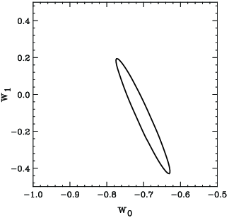
FIG. 1.: The difference in distance modulus between a $k$-essence model defined by $(\Omega_{m},{w_{k}}_{0},{w_{k}}_{1})=(0.3,-0.7,-0.1)$ and the fiducial model $\Omega_{m}=0.3$, $w(z)=-0.7$. The dashed line is the theoretical prediction. The solid line is the best fit to the simulated data with $({w}_{0},{w}_{1})=(-0.7,-0.12)$, demonstrating excellent agreement with the input theory. $\chi^{2}$ is minimized with the assumption that $\Omega_{m}=0.3$ precisely. The $w_{0}-w_{1}$ plane shows the $\Delta\chi^{2}=6.17$ (95.4% confidence level) contour.

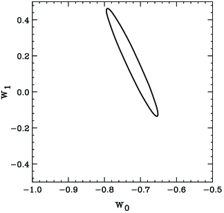
FIG. 2.: The difference in distance modulus between a quintessence model defined by $(\Omega_{m},{w_{Q}}_{0},{w_{Q}}_{1})=(0.3,-0.7,0.1)$ and the fiducial model. The solid line is the best fit (fixing $\Omega_{m}=0.3$) to the simulated data with $({w}_{0},{w}_{1})=(-0.72,0.16)$, demonstrating convincing agreement with the input theory. The $w_{0}-w_{1}$ plane shows the $\Delta\chi^{2}=6.17$ (95.4% confidence level) contour.

Figures  3 and  4 illustrate the crux of our findings that it is also possible for SNAP to obtain datasets that give misleading evidence. Figure 3 shows data generated using a $k$-essence model with $(\Omega_{m},{w_{k}}_{0},{w_{k}}_{1})=(0.3,-0.7,-0.17)$. We chose ${w_{k}}_{1}=-0.17$ so as to allow the equation of state to have the steepest gradient (with ${w_{k}}_{0}=-0.7$) without violating the dominant energy condition $|w_{k}|<1$ for $z<1.7$. Note that $w_{k}(1.7)=-0.99$. The dashed line is the theoretical prediction and the solid line is the best fit with parameters $({w}_{0},{w}_{1})=(-0.79,0.19)$. In minimizing $\chi^{2}$ we have fixed $\Omega_{m}$ at 0.3. We see that the $k$-essence model resembles a quintessence model. It is noteworthy from the $w_{0}-w_{1}$ plane in Fig. 3 that most of the 95.4% confidence contour lies in the region $w_{1}>0$ even though the true model is $k$-essence with $w_{1}<0$. In fact, the contour entirely misses the input theoretical parameters $({w_{k}}_{0},{w_{k}}_{1})=(-0.7,-0.17)$.

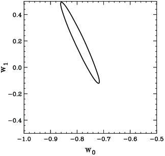
FIG. 3.: The difference in distance modulus between a $k$-essence model defined by $(\Omega_{m},{w_{k}}_{0},{w_{k}}_{1})=(0.3,-0.7,-0.17)$ and the fiducial model. The best fit to the simulated data is $({w}_{0},{w}_{1})=(-0.79,0.19)$, matching a quintessence model. $\chi^{2}$ is minimized with the assumption that $\Omega_{m}=0.3$ precisely. The $w_{0}-w_{1}$ plane shows that the $\Delta\chi^{2}=6.17$ (95.4% confidence level) contour lies mainly in the upper half-plane and does not include the theoretical model.

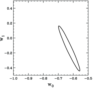
FIG. 4.: The difference in distance modulus between a quintessence model defined by $(\Omega_{m},{w_{Q}}_{0},{w_{Q}}_{1})=(0.3,-0.7,0.2)$ and the fiducial model. The best fit with the assumption that $\Omega_{m}=0.3$ precisely is $({w}_{0},{w}_{1})=(-0.63,-0.14)$ matching a $k$-essence model. The 95.4% confidence level contour lies mainly in the lower half-plane and excludes the theoretical model.

Figure 4 shows results for a quintessence model that looks like a $k$-essence model. The theoretical parameters are $(\Omega_{m},{w_{Q}}_{0},{w_{Q}}_{1})=(0.3,-0.7,0.2)$ and the best-fit parameters are $({w}_{0},{w}_{1})=(-0.63,-0.14)$ keeping $\Omega_{m}=0.3$ during minimization. The 95.4% confidence level excludes the theoretical model $({w_{Q}}_{0},{w_{Q}}_{1})=(-0.7,0.2)$ and lies mainly in the lower half-plane.

Although Figs. 3 and 4 present a discouraging situation, the probability of a dataset conspiring to create the confusion that we have illustrated is not very large. In Fig. 5 we show the percentage of datasets simulated using a given theoretical model as defined by ${w_{k}}_{1}$ or ${w_{Q}}_{1}$ ($\Omega_{m}=0.3$ and $w(0)=-0.7$ for all models) that have best fits (keeping $\Omega_{m}=0.3$ fixed) that conflict with the type of input theory. In making these plots we generated $10^{5}$ datasets for each $w_{1}$ subject only to the assumptions that the dominant energy condition $|w(z)|<1$ be satisfied out to redshift 1.7, and that the value of the equation of state today be less than $-0.6$. The datasets of Figs. 3 and 4 have less than a 1% chance of occurring. However, this does not mean that this sort of misrepresentation by the data is that unlikely to occur. If the equation of state of dark energy does not have a steep gradient, as is necessary if the dark energy is $k$-essence and $w(0)$ is say $-0.8$, then to distinguish between the two theories becomes more difficult than in the examples considered. Moreover, additional degeneracy entering via uncertainties on $\Omega_{m}$ will contribute to confusion in the interpretation of SNAP data. It has been argued [16] that the inability to discriminate between the theories is a consequence of an inefficient fitting function, but the ambiguity is theoretical and cannot be evaded. As shown in Ref. [13], $d_{L}(z)$ depends on $w(z)$ through a multiple-integral relation thus precluding the possibility of a very precise measurement of $d_{L}$ leading to an accurate determination of $dw/dz$.

Even though supernova data may find it difficult to differentiate between quintessence and $k$-essence, CMB anisotropy may be able to detect a smoking-gun signal for $k$-essence because the speed of sound of $k$-essence is not unity as in quintessence models and may lead to peculiarities in the power spectrum not considered so far [11].

FIG. 5.: The percent of datasets derived from $k$-essence models (for different values of ${w_{k}}_{1}$) that have fits with a positive $w_{1}$ is shown on the left. The percent of datasets from quintessence models (for different values of ${w_{Q}}_{1}$) that have negative $w_{1}$ is shown on the right. Only fits yielding $-1\leq w_{0}\leq-0.6$ and $|w(z)|<1$ for $z<1.7$ are allowed. $\Omega_{m}$ is fixed to be $0.3$, and all theoretical models have $w(0)=-0.7$. The number of simulated datasets for each ${w_{k}}_{1}$ (${w_{Q}}_{1}$) is $10^{5}$.

Acknowledgments: This work was supported in part by a DOE grant No. DE-FG02-95ER40896 and in part by the Wisconsin Alumni Research Foundation.

REFERENCES

- [1] N. Bahcall, J. Ostriker, S. Perlmutter and P. Steinhardt, Science 284, 1481 (1999).
- [2] S. Perlmutter, et al., Astrophys. J. 483, 565 (1997).
- [3] A. Riess, et al., Astrophys. J. 116, 1009 (1998).
- [4] S. Perlmutter, et al., Astrophys. J. 517, 565 (1999).
- [5] B. Ratra and P. Peebles, Phys. Rev. D37, 3406 (1988); P. Peebles and B. Ratra, Astrophys. J. 325, L17 (1988).
- [6] J. Frieman, C. Hill, A. Stebbins and I. Waga, Phys. Rev. Lett. 75, 2077 (1995); K. Coble, S. Dodelson and J. Frieman, Phys. Rev. D55, 1851 (1995); C. Wetterich, Astron. Astrophys. 301, 32 (1995); M. Turner and M. White, Phys. Rev. D56, 4439 (1997); P. Ferreira and M. Joyce, Phys. Rev. Lett. 79, 4740 (1997); Phys. Rev. D58, 023503 (1998); E. Copeland, A. Liddle and D. Wands, Phys. Rev. D57, 4686 (1998);
- [7] R. Caldwell, R. Dave and P. Steinhardt, Phys. Rev. Lett. 80, 1582 (1998).
- [8] I. Zlatev, L. Wang and P. Steinhardt, Phys. Rev. Lett. 82, 896 (1999); P. Steinhardt, L. Wang and I. Zlatev, Phys. Rev. D59, 123504 (1999).
- [9] C. Armendariz-Picon, T. Damour and V. Mukhanov, Phys. Lett. B458, 209 (1999).
- [10] T. Chiba, T. Okabe and M. Yamaguchi, Phys. Rev. D62, 023511 (2000).
- [11] C. Armendariz-Picon, V. Mukhanov and P. Steinhardt, astro-ph/0004134; astro-ph/0006373.
- [12] S. Perlmutter, M. Turner and M. White, Phys. Rev. Lett. 83, 670 (1999); D. Huterer and M. Turner, Phys. Rev. D60, 081301 (1999); T. Nakamura and T. Chiba, MNRAS,306, 696 (1999); G. Efstathiou, MNRAS,310, 842 (1999); A. Starobinsky, JETP Lett. 68 757 (1998); S. Podariu and B. Ratra, Astrophys. J. 532, 109 (2000); S. Podariu, P. Nugent and B. Ratra, astro-ph/0008281.
- [13] I. Maor, R. Brustein and P. Steinhardt, astro-ph/0007297.
- [14] T. Saini, S. Raychaudhury, V. Sahni and A. Starobinsky, Phys. Rev. Lett. 85, 1162 (2000).
- [15] T. Chiba and T. Nakamura, astro-ph/0008175.
- [16] J. Weller and A. Albrecht, astro-ph/0008314.
- [17] Y. Wang, Astrophys. J. 531, 676 (2000).
- [18] http://snap.lbl.gov
- [19] J. A. Tyson, D. Wittman and J. R. Angel, astro-ph/0005381.
- [20] C. Lineweaver, Astrophys. J. Lett. 505, L69 (1998); K. Coble et al., ibid 519, L5 (1999); P. de Bernardis et al., Nature 404, 955 (2000).
- [21] P. Binetruy, Phys. Rev. D60, 06350 (1999); Ph. Brax and J. Martin, Phys. Lett. B468, 40 (1999). A. Albrecht and C. Skordis, Phys. Rev. Lett. 84, 2076 (2000); T. Barreiro, E. Copeland and N. Nunes, Phys. Rev. D61, 127301 (2000).