First Structure Formation:
A Simulation of Small Scale Structure at High Redshift

Abstract

We describe the results of a simulation of collisionless cold dark matter in a $\Lambda$CDM universe to examine the properties of objects collapsing at high redshift ($z=10$). We analyze the halos that form at these early times in this simulation and find that the results are similar to those of simulations of large scale structure formation at low redshift. In particular, we consider halo properties such as the mass function, density profile, halo shape, spin parameter, and angular momentum alignment with the minor axis. By understanding the properties of small scale structure formation at high redshift, we can better understand the nature of the first structures in the universe, such as Population III stars.

1 Introduction

The formation of the first stars in the universe, also known as Population III stars because of their lack of metals, is important for many reasons. These objects are responsible for the creation and dispersal of the first metals in the universe via Type II supernovae. The ultraviolet radiation from these first stars may also be partly responsible for the ionization of the intergalactic medium (Haiman, Rees, & Loeb (1997)). These first objects are also the building blocks for the creation of larger structures such as galaxies in the bottom-up model of hierarchical structure formation.

Various workers have studied the process of star formation in the early universe using numerical simulations of metal-free gas. Spherically symmetric simulations are useful because they are computationally less intensive than three dimensional calculations and so can include more physics, such as detailed chemistry and cooling and even radiative transfer (Haiman, Thoul & Loeb (1996); Omukai & Nishi (1998)). However, to follow the collapse of matter to stellar densities, one needs a fully three dimensional approach. Several groups have carried out such simulations including the relevant chemistry (Abel, Bryan, & Norman (2000); Bromm, Coppi & Larson (1999)).

These studies have focused on the evolution of individual density peaks, ignoring the effects of other matter in the universe. Tidal torques impart angular momentum to collapsing objects, affecting their subsequent evolution. Virialized halos can merge, changing the structure of objects. In this paper, we model a relatively large volume, $1\>h^{-1}$Mpc (comoving), that contains a substantial number of halos, in order to understand the nature of the first objects that collapse on a more statistical level.

Since we are interested in the gravitational behavior of the matter, we can model the evolution with an N-body simulation. This is a valid approximation for a universe where collisionless cold dark matter dominates. In such a universe, the gas is coupled to the dark matter, so that gas falls into the potential wells of dark matter halos which may in turn lead to star formation. Thus, we can gain some understanding of the sites of the formation of the first stars via simulations of dark matter.

Thus far, numerical simulations with dark matter have focused on the problem of large scale structure formation (e.g. Efstathiou, et al. (1988); Katz, Hernquist, & Weinberg (1999); Kauffman, et al. (1999); Lacey & Cole (1994)). These simulations address the question of structure formation on the scale of galaxy clusters in order to understand the processes of galaxy formation and clustering. Here, we apply the analytic tools that these groups have developed to address the question of structure formation on a smaller scale.

This paper describes the properties of collapsed objects in a numerical simulation at high redshift and small scales in a $\Lambda$CDM universe. These objects are some of the first non-linear structures in the universe. The non-linear evolution of the power spectrum has been addressed separately (Jang-Condell & Hernquist (2000)). In §2, we summarize the computational method used for the simulation; in §3, we describe the results of the simulation; and in §4 we summarize our results and discuss them in comparison to previous work with N-body simulations.

2 Method

In this simulation, we model the evolution of dark matter in a periodic cube of size $1\>h^{-1}$Mpc per edge in comoving coordinates. We adopt a $\Lambda$CDM cosmology, with $\Omega_{m}=0.35$, $\Omega_{\Lambda}=0.65$, and $h=0.65$, where the Hubble constant is $H_{0}=100h\>$km/s/Mpc. The power spectrum is normalized to $\sigma_{8}=0.9$, where $\sigma_{8}$ is the rms density variation smoothed with a top-hat filter of radius $8\>h^{-1}$Mpc. For the cosmological model we consider, this normalization is roughly consistent with both the local abundance of rich clusters (White, Efstathiou, & Frenk (1993)) and fluctuations in the cosmic microwave background as observed by COBE (Bennett, et al. (1996)).

Initial conditions were generated using the analytic fit to the CDM power spectrum derived by Efstathiou, Bond, & White (1992)

$$P(k)=|\delta_{k}|^{2}=\frac{Bk}{\{1+[ak+(bk)^{3/2}+(ck)^{2}]^{\nu}\}^{2/\nu}}{}\>,$$ (1)

where $a=6.4/\Gamma\>h^{-1}$Mpc, $b=3.0/\Gamma\>h^{-1}$Mpc, $c=1.7/\Gamma\>h^{-1}$Mpc, $\nu=1.13,$ and $B$ is a normalization constant determined by $\sigma_{8}$. The shape parameter $\Gamma$ is set to $\Gamma=\Omega_{m}h$ for a $\Lambda$CDM cosmology. This power spectrum is extrapolated to a starting redshift of 100 assuming linear theory, and is then converted into spatial density fluctuations by first assigning random phases to the $\delta_{k}$ and then taking the Fourier transform. The spatial density fluctuations are converted into particle positions and velocities using the Zel’dovich approximation.

The code used for the simulation is PTreeSPH, a gravity treecode with smoothed particle hydrodynamics (SPH) designed to run on a parallel supercomputer (Davé, Dubinski, & Hernquist 1997). The SPH part of the code was unused in this simulation since gas was not included. The code uses a Barnes-Hut (Barnes & Hut (1986), Hernquist (1987)) algorithm for computational efficiency in calculating gravitational forces and a spline kernel for gravitational softening (Hernquist & Katz (1989)). The softening length chosen for this simulation was $1/20$th of the mean interparticle separation, or $1/2560$th of the box size. The simulation box contains $128^{3}$ particles, implying that each particle represents $4.6\times 10^{4}M_{\sun}$ of dark matter. The simulation was run on a four-processor Beowulf-type cluster of PCs at the Harvard-Smithsonian Center for Astrophysics.

3 Results

The particle distribution at the final output of redshift $z=10$ is shown in Fig. 1. The particles are displayed in projection along the $x$-axis and the colors indicate the particle densities. Already at this high redshift there is evidence of structure formation in the form of clumps and filaments of high particle density. The structures are similar to those seen in large scale simulations evolved to much lower redshift.

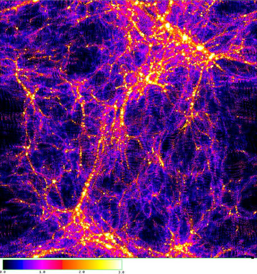
Figure 1: Simulation output at redshift $z=10$. The particles are shown in projection along the $x$-axis. Color indicates log density in units of $\bar{\rho}$. The size of the box is $1\>h^{-1}$Mpc (comoving) per side. (This figure is also available at http://cfa-www.harvard.edu/~hjang/research/prettypic.gif )

As we can see in Fig. 1, the centers of dense knots have densities of $\gtrsim 1000\bar{\rho}$. Density evolves with redshift as $a^{-3}=(1+z)^{3}$, so at $z=10$, $1000\bar{\rho}=1000a^{-3}\Omega_{b}\rho_{\mathrm{crit}}$ where $\Omega_{b}$ is the baryon density of the universe in units of the critical density, and $\rho_{\mathrm{crit}}$ is the present day critical density. Constraints on light element production during big bang nucleosynthesis indicate that $0.01\lesssim\Omega_{b}h^{2}\lesssim 0.015$ (e.g. Peacock (1999), §9.5). Thus,

$$1000\bar{\rho}\approx 3\times 10^{-25}\>\mathrm{g\>cm}^{-3}$$ (2)

which is $\sim 0.2\>\mathrm{cm}^{-3}$ in hydrogen atoms. This is comparable to the density of neutral hydrogen in the present day ISM, which is $\sim 1\>\mathrm{cm}^{-3}$ (e.g. Spitzer (1978), §1.1). We can see that the densest regions in the simulation will be similar in density to the present-day ISM, and so are potential sites for star formation.

3.1 Finding halos

The particle distribution was analyzed using a program called skid to determine the positions, masses, and sizes of collapsed halos. A description of skid can be found at http://www-hpcc.astro.washington.edu/tools/SKID/.

The basic algorithm that skid uses is as follows:

1. Calculate densities, and consider only those above a user specified density threshold. These are called the moving particles.

2. Slide the moving particles along the density gradient toward higher density.

3. Continue moving particles until all the particles stop moving and are localized in high density regions of a user specified size (eps).

4. Group together these localized particles using the friends-of-friends method with a linking-length of eps.

5. Reject groups with less than a user specified minimum number of particles.

6. Particles which are not bound to their group are removed from the group.

7. Reject groups with less than minimum number of particles.

We used a density threshold of $200\bar{\rho}$, a linking-length (eps) of $1/640$th of the box size or 1/5 the mean interparticle spacing, and a minimum halo size of eight particles. Using the simulation output at a redshift of $z=10$, this resulted in 2881 halos, with the largest halo consisting of 8475 particles, corresponding to a mass of $4\times 10^{8}M_{\sun}$ and the smallest with eight particles, corresponding to $4\times 10^{5}M_{\sun}$. The density cutoff was chosen somewhat arbitrarily, and changing its value does not significantly affect the overall results presented in this paper. For example, changing the density threshold from $200\bar{\rho}$ to $86\bar{\rho}$ did not alter the ensemble properties of the halos. Some of the halos identified by skid were subsequently rejected from the sample for being unbound, as described in §3.3. We have analyzed various properties of these halos and describe our results below.

3.2 Mass function

The distribution of halos masses can be expressed in terms of the mass function, $f(M)$, where $f(M)dM$ is the number density of halos of with mass between $M$ and $M+dM$. An analytic prediction for the mass function can be obtained using the Press-Schechter formalism (Press & Schechter (1973)).

The Press-Schechter formalism states that the fraction of the universe condensed into objects of mass $>M$ is

$$F(>M)=1-\mathrm{erf}\left(\frac{\delta_{c}}{\sqrt{2}\,\sigma(M)}\right)$$ (3)

where $\sigma(M)$ is the rms density fluctuation smoothed over spheres of mass $M$, and $\delta_{c}$ is the critical overdensity. The critical overdensity is defined as follows: an object of density $\rho$ in a universe of average density $\bar{\rho}$ is collapsed when

$$\delta=\frac{\rho-\bar{\rho}}{\bar{\rho}}>\delta_{c}.$$ (4)

We take $\delta_{c}=1.69$, the canonical value. The mass function then becomes

$$f(M)\,dM=\left|\frac{dF}{dM}\right|\frac{\bar{\rho}}{M}\,dM=\sqrt{\frac{2}{\pi}}\,\frac{\delta_{c}}{\sigma}\,\bar{\rho}\left|\frac{d\;\ln\sigma}{d\;\ln M}\right|\exp\left(-\frac{\delta_{c}^{2}}{2\sigma^{2}}\right)\,\frac{dM}{M^{2}}.$$ (5)

Figure 2 shows the actual mass function of halos in the simulation compared to the predictions of the Press-Schecter formalism. Halos with positive binding energy were omitted from the calculation of the mass function as explained in Section 3.3. The results are in remarkably close agreement with the Press-Schechter prediction.

Figure 2: Mass function of halos. The points represent the simulation data and the solid line is the Press-Schechter prediction, with $\delta_{c}=1.69$.

3.3 Halo energies

When skid calculates halos from the particle distributions, it removes unbound particles from the halos, so in principle, each halo should be gravitationally bound. The binding energy of particle $i$ to the rest of the halo is

$$E_{i}=m_{i}\left[\frac{1}{2}v_{i}^{2}+\sum_{j\neq i}\Phi_{j}(r_{ij})\right]$$ (6)

where $m_{i}$ and $m_{j}$ are the masses of particle $i$ and particle $j$ respectively, $v_{i}$ is the velocity of particle $i$ with respect to the halo center of mass velocity, and $\Phi_{j}(r_{ij})$ is the gravitational potential between particles $i$ and $j$. The gravitational potential has the general form $\Phi_{j}(r_{ij})=-Gm_{j}f(r_{ij})$, which admits a softened potential for particles pairs with small $r_{ij}$ (Hernquist & Katz (1989)).

The requirement for binding is that $E_{i}<0$. The binding energy for the halo as a whole is the sum of its gravitational potential energy and its kinetic energy. Thus,

$$E=K+W=\frac{1}{2}\sum_{i}m_{i}v_{i}^{2}-\frac{1}{2}\sum_{i}\sum_{i\neq j}Gm_{i}m_{j}f(r_{ij}).$$ (7)

The factor of $\frac{1}{2}$ in the potential energy is to account for double-counting the interactions between pairs of particles. Equation (7) can be rewritten as

$$E=\sum_{i}E_{i}+\frac{1}{2}\sum_{i}\sum_{i\neq j}Gm_{i}m_{j}f(r_{ij})=\sum_{i}E_{i}+|W|$$ (8)

which is greater than the sum of the individual binding energies of the particles. In other words, it is possible to have a halo where each particle is bound to the sum of all the other particles, but the halo as a whole is unbound. So, after skid has calculated the halos, the total binding energy of each halo is checked, and discarded from the sample if it is unbound. Out of the total of 2881 halos, 380 were rejected in this way, leaving 2501 bound halos.

Figure 3: Distribution of unbound halos with respect to halo size in terms of particle number.

The distribution in size of the 380 unbound halos is plotted in Figure 3. Note that the unbound halos are all quite small, the largest containing only 25 particles. This shows that our method of using skid to calculate halos is fairly robust, failing only at small halo sizes, which are intrinsically unstable to small perturbations. In the analysis of the remaining halo properties, calculations are done either as a function of mass, or neglecting all halos with less than 50 particles. Thus, the removal of these halos from the sample will not significantly affect our results.

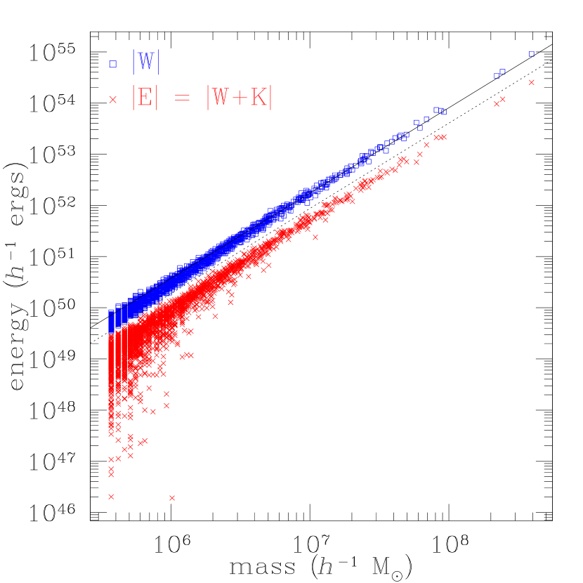
Figure 4: Energies of the halos versus mass. Potential energy is plotted as squares, total binding energy is plotted as crosses. The solid line is proportional to $M^{5/3}$.

Figure 4 is a plot of the energies of the halos versus their masses. The absolute values of the potential energy are plotted as squares and the absolute values of the total binding energy are plotted as crosses. The energies all seem to follow a power law of $E\propto M^{5/3}$, as indicated by the solid line. This relation can be obtained analytically by supposing that the halos are the result of the collapse of spheres of uniform density. This is a reasonable assumption since the universe was initially very nearly uniform in density. If the density is constant, then the mass of a sphere of radius $r$ is

$$M(r)=\frac{4\pi\rho}{3}r^{3}.$$ (9)

The equation for the gravitational potential energy energy of a uniform sphere of density $\rho$ and mass $M$ is

$$W = \int_{0}^{R}\Phi(r)\rho\,d^{3}r$$ (10)

$$= \int_{0}^{R}-\frac{GM(r)}{r}\,\rho\,4\pi r^{2}dr$$

$$= -\frac{3GM^{2}}{5R}$$

$$= -\frac{3}{5}GM^{5/3}\left(\frac{4\pi\rho}{3}\right)^{1/3}.$$

Assuming that the halo is virialized, we have

$$E=K+W=-\frac{1}{2}W+W=\frac{1}{2}W.$$ (11)

Thus, the total energy should obey the same scaling.

The dotted line represents $1/2$ the energy of the solid line. The total energies of the halos are all below this line, indicating that $E>\frac{1}{2}W$ in general. This means that the halos have not yet become virialized. This is also shown in Fig. 5, which shows the ratio between the kinetic energy and the potential energy. The solid line marks $K=\frac{1}{2}|W|$, which would indicate a virialized halo. Nearly all the halos have too high a kinetic energy for virialization.

Figure 5: Ratio of kinetic to potential energy. The solid line indicates $K=\frac{1}{2}|W|$, which holds for virialized objects.

3.4 Gas temperature

Assuming that the matter in the universe is dominated by cold dark matter, then the gas should trace the distribution of the dark matter. In particular, gas should fall into the potential wells of the dark matter halos and become shock heated to the virial temperature of the halo. We can estimate this temperature by assuming that the mean-square velocity of the gas is the same as the dark matter.

For an ideal gas, the temperature is related to the mean-square velocity by

$$\langle v^{2}\rangle=\frac{3kT}{\mu m_{p}},$$ (12)

where $k$ is Boltzmann’s constant, $T$ is the temperature in Kelvin, $m_{p}$ is the proton mass, and $\mu$ is the mean molecular weight. This temperature, as a function of $\mu$, is plotted versus mass for each halo in Fig. 6. The value of $\mu$ will depend on the composition and ionization state of the gas.

As discussed in section 3.3, the kinetic energy of the halo follows a power law of $K\propto M^{5/3}$. Since $K=\frac{1}{2}M\langle v^{2}\rangle$, the temperature should follow the relation

$$T\sim M^{2/3}.$$ (13)

This is indicated by the solid line in Fig. 6. The temperatures follow this power law relation fairly well.

Figure 6: Virial temperature versus mass. The solid line is proportional to $M^{2/3}$.

3.5 Halo profiles

We calculated the density profiles of the thirty most massive halos. The spherically averaged density as a function of radius for these halos, with the potential minimum as the center, is plotted in Figs. 7 and 8. The potential minimum was chosen over the center of mass because the potential minimum is more likely to be at the point of highest density.

Possible analytic fits to dark matter halo profiles are those due to Hernquist (1990) and Navarro, Frenk & White (1997, henceforth NFW). Avila-Reese, et al. (1999) proposed the following general form for the fitting formulae:

$$\rho(r)=\frac{\rho_{0}}{\frac{r}{r_{s}}\left(1+\frac{r}{r_{s}}\right)^{\beta-1}}$$ (14)

where $\rho_{0}$ and $r_{s}$ are scalings for the density and radius, respectively, and $\beta$ is a power-law index parameter explained as follows. When $\beta=4$ this corresponds to a Hernquist profile, and when when $\beta=3$ this corresponds to an NFW profile. We can also allow $\beta$ to be a free parameter. The asymptotic behavior of the profiles is

$$\rho\sim\left\{\begin{array}[]{ll}r^{-1},&r/r_{s}\ll 1\\ r^{-\beta},&r/r_{s}\gg 1.\\ \end{array}\right.$$ (15)

Thus, $\beta$ parametrizes the profile shape at at radii much larger than the scale length.

The fits to the NFW and Hernquist profiles are indicated in Figs. 7 and 8 by dotted and short dashed lines, respectively. A third model, allowing $\beta$ to be a free parameter in the fit, is indicated by a long dashed line. This fitted $\beta$ is displayed at the bottom of each profile plot. The scale radius $r_{s}$ for each of these three profiles is indicated by filled, fat, and thin triangles, respectively.

All three profiles are good fits to the data, and are indistiguishable. This is because the power-law slopes for all the halos are fairly close to $-2$. Since each profile is a smoothly varying function, the power-law slope also varies smoothly from $-1$ to $-\beta$. One can easily fit the part of the profile with power-law slope $-2$ to each halo profile. Note also that $\beta\sim 3.5$ in all cases, intermediate to the NFW and Hernquist profile expectations. The close agreement of the fits can also be explained by the relatively large values of $r_{s}$ with respect to the sizes of the halos. The halos are only a few scale radii in size, so we are well below the regime where the halo profiles behave as $\rho\propto r^{-\beta}$.

Figure 7: Density profiles of halos. Radius is in physical parsecs. Dotted line is NFW profile fit, short dashed line is Hernquist profile fit, and long dashed line is the fit allowing $\beta$ to be a free parameter. Triangles mark the $r_{s}$ for each fitted profile – solid triangle is NFW, hollow triangle is Hernquist, and deflated triangle is the best-fit $\beta$ profile.

Figure 8: Same as Fig. 7.

3.6 Spin parameter

The spin parameter of a bound object is defined as

$$\lambda=\frac{J|E|^{1/2}}{GM^{5/2}}$$ (16)

where $J$ is the angular momentum, $E=K+W$ is the binding energy, $G$ is the gravitational constant, and $M$ is the mass. This is a dimensionless parameter that quantifies the amount of rotational support an object has. A value of $\lambda\sim 1$ corresponds to nearly full rotational support, and is typical of spiral galaxies, while $\lambda\sim 0.05$ is typical of elliptical galaxies, which are supported by velocity dispersion. Figure 9 is a plot of spin parameter versus mass for the halos in the simulation.

Figure 9: Spin parameter versus mass.

Mo, Mao & White (1998) found that the distribution of spin parameters of dark matter halos in galaxy formation simulations approximates a log-normal distribution, that is

$$p(\lambda)\,d\lambda=\frac{1}{\sqrt{2\pi}\sigma}\exp\left[-\frac{\ln^{2}(\lambda/\bar{\lambda})}{2\sigma^{2}}\right]\,\frac{d\lambda}{\lambda}.$$ (17)

with fitting parameters of $\bar{\lambda}=0.05$ and $\sigma_{\lambda}=0.5$. The log-normal distribution is also a good fit for the data presented in this paper, as shown in Fig. 10. The simulation data is displayed as squares, and the log-normal fit to it is the solid line. The fitting parameters are $\bar{\lambda}=0.043$ and $\sigma_{\lambda}=0.53$, which is consistent with the results of Mo, Mao & White (1998).

The smallest halos in the simulation contain only eight particles. For a halo with so few particles, the spin parameter is not a particularly meaningful quantity. Since the most numerous halos in the simulation are the smallest ones, the distribution of $\lambda$ calculated above may not be particularly meaningful either. We recalculated the distribution of $\lambda$ for halos containing at least $50$ particles to determine the effect of excluding small halos. This is plotted as diamonds in Fig. 10, and the log-normal fit to it is the dashed line. The fitting parameters for these 389 halos is $\bar{\lambda}=0.033$ and $\sigma_{\lambda}=0.52$, indicating that the larger halos have systematically smaller spin parameters than smaller halos.

Figure 10: Distribution of spins. The squares and diamonds show the normalized distribution for all the halos and halos with at least 50 particles, respectively. The solid line and the dashed line show the log-normal fit to the respective data sets.

3.7 Halo shapes

A typical dark matter halo is not actually spherical, but is triaxial due to anisotropy in its velocity dispersion. Thus, the shape of a halo can be quantified by finding its best fitting ellipsoid. The three axes of the best fitting ellipsoid will be referred to as the major, intermediate, and minor axes, in decreasing order of size.

3.7.1 Method of calculating ellipsoids

The best-fitting ellipsoid can be found by using the moment of inertia tensor, which is defined as

$$\mathbf{I} = \left[\begin{array}[]{ccc}\sum\limits_{i}m_{i}(y_{i}^{2}+z_{i}^{2})&-\sum\limits_{i}m_{i}x_{i}y_{i}&-\sum\limits_{i}m_{i}x_{i}z_{i}\\ -\sum\limits_{i}m_{i}y_{i}x_{i}&\sum\limits_{i}m_{i}(x_{i}^{2}+z_{i}^{2})&-\sum\limits_{i}m_{i}y_{i}z_{i}\\ -\sum\limits_{i}m_{i}z_{i}x_{i}&-\sum\limits_{i}m_{i}z_{i}y_{i}&\sum\limits_{i}m_{i}(x_{i}^{2}+y_{i}^{2})\\ \end{array}\right]$$ (21)

$$= \sum_{i}m_{i}\left(\left[\begin{array}[]{ccc}r_{i}^{2}&0&0\\ 0&r_{i}^{2}&0\\ 0&0&r_{i}^{2}\\ \end{array}\right]-\left[\begin{array}[]{ccc}x_{i}^{2}&x_{i}y_{i}&x_{i}z_{i}\\ y_{i}x_{i}&y_{i}^{2}&y_{i}z_{i}\\ z_{i}x_{i}&z_{i}y_{i}&z_{i}^{2}\\ \end{array}\right]\right)$$ (28)

$$= \sum_{i}m_{i}(r_{i}^{2}\mathbf{1}-\mathbf{r}_{i}\mathbf{r}_{i})$$ (29)

where $r_{i}=\sqrt{x_{i}^{2}+y_{i}^{2}+z_{i}^{2}}$ is the distance of the $i$th particle to the center of the distribution of particles. The moment of inertia $I$ about an axis through the center of the distribution in the direction of the unit vector $\mathbf{n}$ is given by

$$I=\mathbf{n}\cdot\mathbf{I}\cdot\mathbf{n}.$$ (30)

Another property of the moment of inertia tensor is that the angular momentum $\mathbf{L}$ can be expressed as

$$\mathbf{L}=\mathbf{I}\cdot\mathbf{\omega}.$$ (31)

Thus, the eigenvectors correspond to the axes about which the angular velocity and angular momentum are aligned and the eigenvalues are the corresponding moments of inertia.

Consider an ellipsoid of constant density centered at the origin with its axes along the $x$-, $y$-, and $z$-axes defined by

$$\frac{x^{2}}{a^{2}}+\frac{y^{2}}{b^{2}}+\frac{z^{2}}{c^{2}}\leq 1.$$ (32)

By symmetry, the moment of inertia tensor is already diagonalized, and the diagonal elements are the eigenvalues. It can be shown (through some rather tedious integration) that the diagonal elements are

$$I_{1} = \frac{M}{5}(b^{2}+c^{2})$$

$$I_{2} = \frac{M}{5}(a^{2}+c^{2})$$

$$I_{3} = \frac{M}{5}(a^{2}+b^{2})$$

where $M$ is the total mass of the ellipsoid. Using equation (21), we now have

$$\frac{M}{5}\left[\begin{array}[]{ccc}(b^{2}+c^{2})&0&0\\ 0&(a^{2}+c^{2})&0\\ 0&0&(a^{2}+b^{2})\\ \end{array}\right]=\frac{M}{5}(a^{2}+b^{2}+c^{2})\mathbf{1}-\sum_{i}m_{i}\mathbf{r}_{i}\mathbf{r}_{i}$$ (34)

which reduces to

$$\sum_{i}m_{i}\mathbf{r}_{i}\mathbf{r}_{i}=\frac{M}{5}\left[\begin{array}[]{ccc}a^{2}&0&0\\ 0&b^{2}&0\\ 0&0&c^{2}\\ \end{array}\right].$$ (35)

Thus, the axes of the best fitting ellipsoid can found by calculating the tensor

$$M_{\alpha\beta}=\sum_{i}m_{i}x_{\alpha,i}x_{\beta,i}$$ (36)

and finding its eigenvalues and eigenvectors.

The simplest way of determining the halo shape is to use the center of mass as the center of the distribution and to sum over all the particles in the halo to calculate the tensor $M_{\alpha\beta}$. However, some halos found by the skid program include satellite halos or consist of two or more groups connected by a thin bridge. The center of mass for these halos may not actually lie in the center of the halo. In addition, ellipsoids calculated about the center of mass have systematically higher axial ratios – that is, they are more spheroidal in shape. This can be explained by the fact that skid tends to calculate halos within a spherical volume, regardless of the intrinsic shape of the halo. Thus, the calculated shape of the halo is more rounded out, so to speak.

A better approximation is to use the potential minimum as the center of the distribution and to sum over the inner part of the halo. We used an iterative method to fit an ellipsoid to half the mass of the halo. The procedure begins by finding the sphere centered at the potential minimum that contains half the mass of the halo. These particles are used to calculate an initial guess for the ellipsoid axes. Keeping the orientation and axial ratios of the ellipsoid fixed, a new ellipsoid is calculated which contains half the mass of the halo. The particles within this ellipsoid are used to calculate a new $M_{\alpha\beta}$ and a new guess for the ellipsoid is calculated. This procedure is repeated until the values of the axes converge. Dubinski and Carlberg (1991) employed a similar method to calculate halo shapes, but using particles within a fixed distance of the halo center rather than a fixed fraction of the mass. In order to leave out halos that are too small to have their shapes accurately calculated, we chose a lower cutoff to the halo size of 50 particles. There were 389 halos of this size.

3.7.2 Ellipticities and triaxiality

Using the iterative procedure described above, we calculated the magnitude and orientation of the principal axes of each halo. Henceforth, we shall refer to the lengths of the major, intermediate, and minor axes as $a$, $b$, and $c$, respectively. The ellipticities of the halos,

$$\epsilon_{1} = 1-b/a,$$

$$\epsilon_{2} = 1-c/b,$$

are useful measures of the shapes. A perfectly spherical halo would have $a=b=c$, hence $\epsilon_{1}=\epsilon_{2}=0.$ An oblate halo would have the larger two axes equal to each other ($a=b$), hence $\epsilon_{1}=0$ and $\epsilon_{2}>0$. A prolate halo would have the smaller two axes equal to each other ($b=c$), hence $\epsilon_{1}>0$ and $\epsilon_{2}=0$. In general, however, a halo will be triaxial, meaning that there are no equalities between axis lengths.

Figure 11 is a plot showing the ellipticities of the halos. The diagonal line shows the division between prolate and oblate halos – prolate halos lie below the line, and oblate halos lie above it. By this criterion, there are 212 prolate halos and 177 oblate halos. Warren et al. (1992) also found more prolate than oblate halos in their simulations of dark matter halos at zero redshift at galaxy size scales (the smallest mass they considered was $3\times 10^{9}M_{\sun}$). They found this result to be independent of the initial power spectrum used, so it is reassuring that we obtain the same results for our simulation, although we use a different power spectrum and mass range.

We can also compare the prolateness/oblateness of halos by use of the triaxiality parameter $T$, which is defined as

$$T=\frac{a^{2}-b^{2}}{a^{2}-c^{2}}.$$ (37)

A halo that is purely prolate has $b=c$, so $T=1$. A halo that is purely oblate has $a=b$, so $T=0$. The dotted lines in Fig. 11 represent contours of constant $T$.

Figure 12 is a plot of $T$ versus halo mass. There does not appear to be any strong correlation between mass and triaxiality. However, there is a tendency at all masses for the triaxiality to be close to $1$. Figure 13 shows the distribution of the triaxiality parameter for all halos with at least 50 particles. The halos tend toward high values of $T$, another indication that prolate halos dominate. These two figures are qualitatively similar to Figs. 9a and 8 in Warren et al. (1992), indicating that our results are similar to theirs, despite the difference in mass scales and redshift.

Figure 11: Ellipticities of halos of size $\geq 50$ particles, defined as $\epsilon_{1}=1-b/a$ and $\epsilon_{2}=1-c/b$. The dashed line shows the division between prolate and oblate halos, and the dotted lines show contours of constant triaxiality.

Figure 12: Triaxiality of halos with $\geq 50$ particles versus mass.

Figure 13: Distribution of halo triaxiality parameter $T$, defined as $T=(a^{2}-b^{2})/(a^{2}-c^{2})$.

3.7.3 Angular momentum misalignment

Now that we have calculated the axes of the best-fit ellipsoids of the halos, we can consider the orientation with respect to the angular momentum. Since the ellipsoids were fit using half the mass of the halo, we also recalculate the angular momenta using the positions and velocities of the same particles that were used to calculate the ellipsoids. We find the cosine of the angles between the angular momentum and each of the principal axes by taking dot products.

Figure 14 shows the distribution of these angle cosines. The dotted, dashed, and solid lines show the distribution of the angle cosines between the major, intermediate, and minor axes of the halo, respectively. As we can see in Fig. 14, the angular momentum tends to be aligned with the minor axis of halos. This is consistent with observations of elliptical galaxies which indicate that the angular momentum vector tends to align with the the minor axis (Franx, et al. (1991)).

Figure 14: Distribution of angle cosines between angular momentum vector and ellipsoid axes for halos with $\geq 50$ particles. The dotted (dashed, solid) line shows the cosine of the angle between the major (intermediate, minor) axis of the halo.

Kinematically, the angular momentum should align with either the major or minor axis because particles in a triaxial potential admit tube orbits only about these axes. In other words, particles may only circulate about either the major or the minor axis, causing the angular momentum of the system as a whole to align with these axes (Binney & Tremaine (1994)). However, most halos do not show alignment with the major axis. In fact, many have their angular momentum perpendicular to their major axis.

In addition, there are a number of halos whose angular momentum is aligned with the intermediate axis, even though this configuration is kinematically unstable. Warren et al. (1992) also observe this in their dark matter simulations, and suggest that this is caused by a long time scale for the realignment of orbits.

4 Summary

The major conclusion of that paper is that this N-body simulation of small scale structure formation at high redshift is similar to N-body simulations of large scale structure formation at at low redshift. The details can be summarized as follows:

1. The mass function of the halos can be well approximated by the Press-Schechter formalism.

2. The profile of the halos can be modeled equally well by either the NFW and Hernquist profiles.

3. The shapes of the halos are generally triaxial, with a tendency toward prolateness.

4. The average spin parameter of the halos is about $0.04$.

5. The angular momentum tends to align with the minor axis most often, and favors alignment with the intermediate axis over the major axis.

In fact, it would be surprising if the results were completely different from other N-body simulations, since they all model the gravitational collapse of objects from some primordial power spectrum of density fluctuations. The main difference is in the shape of the power spectrum, which changes as we go to smaller scales. This produces a corresponding change in the mass spectrum of objects that are collapsing.

The Press-Schechter formalism predicts how the mass spectrum of collapsed objects depends on the initial power spectrum. We find that the mass function matches the predictions of Press-Schechter remarkably well, even at the low mass end. This is consistent with previous work with N-body simulations at low redshift and large scales which have also shown good agreement with the Press-Schechter formalism (Efstathiou, et al. (1988); Kauffman & White (1993); Lacey & Cole (1994); Valageas, Lacey & Schaeffer (2000)).

The remaining halo properties described in this paper, including density profile, halo shape, and spin parameter, all are consistent with previous work with N-body simulations regardless of the power spectrum used. Some authors use scale invariant power spectra, but using a range of spectral indices: choices of $-2$, $-1$, and $0$ are typical (Cole & Lacey (1996); Warren, et al. (1992)). Some use a CDM spectrum or some variant (Mo, Mao, & White (1998)). Note that at the high redshifts studied in this paper, the dynamical evolution of a $\Lambda$CDM universe is the same as that of a pure CDM universe, since the matter density varies as $(1+z)^{3}$ while the vacuum energy density remains constant. However, the spectral index approaches $\sim-3$ on small scales, so we effectively choose a different power spectrum by considering small scales. Although the initial power spectrum used in this paper is different from previous work, the overall results on halo properties remains the same.

The shapes of the density profiles of the halos are consistent with both NFW and Hernquist profiles, which are based on studies of collapsed halos in cold dark matter simulations. Indeed, when the shape of the outer profile $\beta$ is allowed to be a free parameter, we find that $3<\beta<4$, intermediate to the NFW and Hernquist profiles.

The results for the spin parameter and shapes of halos are also consistent with large-scale structure simulations. The median and distribution of the spin parameter are both similar to the those found for large-scale simulations, i.e. $\bar{\lambda}=0.043$, with a log-normal distribution (Mo, Mao, & White (1998); Cole & Lacey (1996)). The predominance of prolate halo shapes also agrees with these other simulations (Warren, et al. (1992); Cole & Lacey (1996)), as well as the alignment of the angular momentum with the minor axis (Weil & Hernquist (1994); Warren, et al. (1992)). We also find that the angular momentum favors alignment with the intermediate axes over the major axis, as Warren et al. (1992) do.

We can infer from this simulation that dark matter halos on small scales at high redshift behave very similarly to halos on large scales at low redshift. This can help us understand high-redshift star formation by providing information on the dark matter environments in which the first stars formed. Further study using simulations such as this may shed light on the IMF of the first stars, and their subsequent fate. By adding additional physics to the simulation, such as gas physics and radiative transfer, we can study the nature of the first objects that formed in the universe.

This work was supported under an NSF Graduate Fellowship, by NASA Astrophysical Theory Grant NAG5-8727, and by NSF grants ACI96-19019 and AST-9803137.

References

- Abel, Bryan, & Norman (2000) Abel, T., Bryan, G. L., & Norman, M. L. 2000, ApJ, in press (astro-ph/0002135)
- Avila-Reese, et al. (1999) Avila-Reese, V., Firmani, C., Klypin, A., & Kravtsov, A. 1999, MNRAS, 310, 527
- Barnes & Hut (1986) Barnes, J., & Hut, P. 1986, Nature, 324, 446
- Bennett, et al. (1996) Bennett, C. L., et al. 1996, ApJ, 464, L1
- Binney & Tremaine (1994) Binney, J., & Tremaine, S. 1994, Galactic Dynamics (Princeton: Princeton University Press)
- Bromm, Coppi & Larson (1999) Bromm, V., Coppi, P. S., & Larson, R.,B. 1999, ApJ, 527, L5
- Cole & Lacey (1996) Cole, S., & Lacey, C. 1996, MNRAS, 281, 716
- (8) Davé, R., Dubinski, J., & Hernquist, L. 1997, New Astronomy, 2, 277
- Dubinski & Carlberg (1991) Dubinski, J., & Carlberg, R. G. 1991, ApJ, 378, 496
- (10) Efstathiou, G., Bond, J. R., & White, S. D. M. 1992, MNRAS, 258, 1p
- Efstathiou, et al. (1988) Efstathiou, G., Frenk, C. S., White, S. D. M., & Davis, M. 1988, MNRAS, 235, 715
- Franx, et al. (1991) Franx, M., Illingworth, G., & de Zeeuw, T. 1991, ApJ, 383, 112
- Haiman, Rees, & Loeb (1997) Haiman, Z., Rees, M. J., & Loeb, A. 1997, ApJ, 476, 458
- Haiman, Thoul & Loeb (1996) Haiman, Z., Thoul, A. A., & Loeb, A. 1996, ApJ, 464, 523
- Hernquist (1987) Hernquist, L. 1987, ApJS, 356, 359
- Hernquist (1990) Hernquist, L. 1990, ApJ, 64, 715
- Hernquist & Katz (1989) Hernquist, L., & Katz, N. 1989, ApJS, 70, 419
- Jang-Condell & Hernquist (2000) Jang-Condell, H., & Hernquist, L. 2000, MNRAS, submitted
- Katz, Hernquist, & Weinberg (1999) Katz, N., Hernquist, L., & Weinberg, D. H. 1999, ApJ, 523, 463
- Kauffman, et al. (1999) Kauffman, G., Colberg, J. M., Diaferio, A., & White, S. D. M. 1999, MNRAS, 303, 188
- Kauffman & White (1993) Kauffman, G., & White, S. D. M. 1993, MNRAS, 261, 921
- Lacey & Cole (1994) Lacey, C., & Cole, S. 1994, MNRAS, 271, 676
- Mo, Mao, & White (1998) Mo, H. J., Mao, J., & White, S. D. M. 1998, MNRAS, 295, 319
- Navarro, Frenk, & White (1997) Navarro, J. F., Frenk, C. S., & White, S. D. M. 1997, ApJ, 490, 493
- Omukai & Nishi (1998) Omukai, K., & Nishi, R. 1998, ApJ, 508, 141
- Peacock (1999) Peacock, J. A. 1999, Cosmological Physics (Cambridge: Cambridge University Press)
- Press & Schechter (1973) Press, W. H., & Schechter, P. 1973, ApJ, 187, 425
- Spitzer (1978) Spitzer, L. 1978, Physical Processes in the Interstellar Medium (New York: John Wiley & Sons, Inc.)
- Valageas, Lacey & Schaeffer (2000) Valageas, P., Lacey, C., & Schaeffer, R. 2000, MNRAS, 311, 234
- Warren, et al. (1992) Warren, M. S., Quinn, P. S., Salmon, J. K., & Zurek, W. H. 1992, ApJ, 399, 405
- Weil & Hernquist (1994) Weil, M. L., & Hernquist, L. 1994, ApJ, 431, L79
- White, Efstathiou, & Frenk (1993) White, S. D. M., Efstathiou, G., & Frenk, C. S. 1993, MNRAS, 262, 1023