ASCA and other contemporaneous observations of the blazar B2 1308+326
Abstract
The high redshift () blazar B2 1308+326 was observed contemporaneously at x-ray, optical and radio wavelengths in June 1996. The x-ray observations were performed with ASCA. The ASCA results were found to be consistent with reanalysed data from two earlier ROSAT observations. The combined ASCA and ROSAT data reveal an x-ray spectrum that is best fit by a broken power law with absorber model with photon spectral indices of and and a break energy at keV in the rest-frame of the blazar. The break in the x-ray spectrum is interpreted, from the shape of the simultaneous broadband spectral energy distribution, to be the emerging importance of inverse Compton (IC) emission which dominates the ASCA spectrum.The faint optical state reported for these observations (m) is incompatible with the high synchrotron flux previously detected by ROSAT. The IC emission detected by both ROSAT and ASCA was not significantly affected by the large change in the synchrotron component.
Mg ii emission was detected with an equivalent width (Wλ) of 15Å, significantly different from previously reported values. The small and variable Wλ in B2 1308+326 may be due to the highly variable continuum and not intrinsically weak lines in the source. A lower limit on the Doppler boost factor calculated from the contemporaneous data is consistent with expectations for highly polarised quasars and higher than expected for BL Lacs. Absorption at a level of N cm-2 was detected which is in excess of the Galactic value of N cm-2, indicating the possible presence of a foreground absorber. A gravitational microlensing scenario cannot therefore be ruled out for this blazar. No significant variability on timescales of hours was detected in the optical or x-ray data.
B2 1308+326 could be a typical radio-selected BL Lac in terms of peak synchrotron frequency and optical and radio variability but its high bolometric luminosity, variable line emission and high Doppler boost factor make it appear more like a quasar than a BL Lac. It is suggested that B2 1308+326 be considered as the prototype of this class of composite source.
Key Words.:
BL-Lacertae objects: individual: B2 1308+326 – quasars: individual: B2 1308+326 – X-rays: galaxies – Radio continuum: galaxies – gravitational lensing1 Introduction
The classification of the high redshift () source B2 1308+326 is uncertain Gabuzda et al. (1993). It has been designated a BL Lac Stickel et al. (1991) because of its almost featureless optical spectrum Wills & Wills (1979), its strong optical variability Mufson et al. (1985) and the high degree of polarization of its optical continuum Angel & Stockman (1980). As one of the 1 Jy sample of BL Lacs, B2 1308+326 is classified as a Radio-Selected BL Lac (RBL) Stickel et al. (1993).
However, B2 1308+326 also exhibits quasar-like properties. VLBI polarisation images show that the polarised flux from the inner part of the jet is nearly perpendicular to the direction of the jet which is a characteristic property of quasars not BL Lacs Gabuzda et al. (1993). The degree of core polarisation from VLBI observations of B2 1308+326 is somewhat higher than usual for quasars and at the lower end of the range for BL Lacs Gabuzda et al. (1993). Measurements of the apparent speed of knots emerging from the core are superluminal (, , ) and above the typical speeds observed in BL Lacs Gabuzda et al. (1993). B2 1308+326 also shows an optical-UV excess above the IR extrapolation Brown et al. (1989), and its radio power and morphology are FR II (Fanaroff & Riley, 1974, type II) in nature Kollgaard et al. (1992). The FR II classification is not that unusual among BL Lacs Kollgaard et al. (1996), but an FR I morphology would strongly militate against its being a quasar Urry et al. (2000); Kollgaard et al. (1990). The large bolometric Sambruna et al. (1996) and 5 GHz luminosities Kollgaard et al. (1992) are further indications that it could be regarded as a quasar. The term “blazar” is particularly useful for sources like this, encompassing as it does flat spectrum radio quasars (FSRQs) and BL Lacs. It must be noted that the terms highly polarised quasars (HPQs), optically violently variable (OVV) quasars, FSRQs (and more recently, quasar-hosted blazar) are used to refer to blazar subclasses. The significant distinction here is between quasar-type and BL Lac-type blazars and the term FSRQ is used except in cases where another classification occurs in a work cited in the text.
Two main approaches have proven to be effective in constraining models of BL Lacs; monitoring their variability (e.g. Georganopoulos & Marscher 1998a), and studying their broadband spectral energy distributions (SEDs) (e.g. Sambruna et al. 1996, Kubo et al. 1998, Sambruna et al. 1999). Rapid flux variations and changes in the shape of the SEDs of blazars are common (e.g. Pian et al. 1998, Macomb et al. 1995, Chiaberge & Ghisellini 1999). To place adequate constraints on the synchrotron emission (e.g. the Doppler boost factor of the putative jet and the angle between such a jet and the line of sight) in these sources requires simultaneous observations over a wide range of frequencies.
It has been suggested that some sources with BL Lac characteristics are actually gravitationally microlensed quasars Nottale (1986); Ostriker & Vietri (1990). The best candidates include AO 0235+164 Rabbette et al. (1996), PKS 0537-441 Romero et al. (1999) and MS 0205.7+3509 Watson et al. (1999). B2 1308+326 has characteristics intermediate between BL Lacs and quasars. Gabuzda et al. Gabuzda et al. (1993) have therefore suggested that B2 1308+326 may be gravitationally microlensed. Observation of a foreground galaxy would lend support to the argument that it is indeed gravitationally lensed. However high resolution imaging with the HST WFPC2 Urry et al. (1999) did not confirm the detection of spatially extended emission reported by Stickel et al. Stickel et al. (1993). The observations were consistent with a point source with an upper limit of m mag arcsec-2 for any surrounding galaxy.
In the superluminal micro-lensing scenario, the time scale for rapid variability can constrain source parameters (e.g. Lorentz factor and source diameter, McBreen & Metcalfe 1987, Gopal-Krishna & Subramanian 1991). Such microlensing variations should be achromatic and therefore detectable with simultaneous multi-wavelength observations.
Simultaneous x-ray, optical and radio observations were carried out in order to constrain the nature of the emission in B2 1308+326. These observations and the data reduction procedures are described in Sect. 2. Results are presented in Sects. 3 and 4 and are discussed in Sect. 5 with conclusions in Sect. 6. km s-1 Mpc-1 and are assumed throughout.
2 Observations and data reduction
2.1 X-ray observations
Observations of B2 1308+326 were made with the ASCA satellite Tanaka et al. (1994) between 15:26 and 23:41 UT on 10 June 1996, and between 23:37 UT on 11 June 1996 and 09:10 UT on 12 June 1996. There are four instruments on board ASCA, two Gas Imaging Spectrometers (GIS-S2 and GIS-S3) and two Solid-state Imaging Spectrometers (SIS-S0 and SIS-S1). The instruments have a well-calibrated energy range of 0.7–10.0 keV for the GIS and 0.5–10.0 keV for the SIS and only data in these energy ranges were used for spectral fitting. The total exposure time per instrument was approximately 40 ks. The SIS data were recorded in FAINT data mode and converted to BRIGHT-2 mode Inoue (1993) having corrected for the Residual Dark Distribution (RDD) effect with the FTOOLS script ‘Correctrdd’.
Data from the SIS and GIS instruments were screened in a standard way, and were then reduced using the FTOOLS applications. An extraction region was defined around the source, with an aperture of 4′ for the SIS detectors and 6′ for the GIS. This spatial region was used to extract the source plus background counts. An estimate of the background was derived by taking an annulus around the extraction aperture and extracting counts from this region. An alternative background estimate was derived from separate dark-sky observations made by ASCA and results obtained using both types of background estimates were found to be consistent. The annulus background was subtracted from the extracted source plus background counts to obtain a source spectrum. The resulting spectra were rebinned to have a minimum of 20 counts per bin in order to ensure the validity of the Gaussian approximation.
Two observations of the source were made with the ROSAT PSPC Pfeffermann & Briel (1986) on 23 June 1991 Comastri et al. (1995); Lamer et al. (1996) and 3 June 1992. These data were reduced in a standard way using the FTOOLS software. The response matrix from ROSAT AO-1 was used to analyse the data from the 23 June 1991 observation, and that from AO-2 for the 3 June 1992 observation. Only the well-calibrated data between 0.1–2.4 keV were used.
2.2 Optical and radio observations
Optical Johnson V-band observations were carried out under photometric conditions with the 1.23 m telescope at Calar Alto Observatory, Spain on the nights of 10 and 11 June 1996 with typical exposure times of 900 s. Standard CCD aperture photometry techniques were used to reduce the data. Absolute calibration of the source was derived using V-band differential photometry on a calibrated reference star within the CCD field of view (star C from Fiorucci et al. 1998). Optical V-band observations made two weeks later with the 1 m JKT telescope at La Palma Observatory showed the source to be of the same magnitude, within the error of 0.25 mag. The relative uncertainty (0.08 mag.) in the optical magnitude was brought below the absolute calibration uncertainty (0.25 mag.), by using differential photometry techniques Rabbette et al. (1998).
Observations were carried out under non-photometric conditions at the 2.12 m telescope of the Observatorio “Guillermo Haro” at Cananea, Son., México on June 16, 1996 using the Landessternwarte Faint Object Spectrograph and Camera (LFOSC) in 5.5 Å/pixel mode. The standard IRAF utility package distributed by the National Optical Astronomy Observatories was used to reduce the data. The spectral images were processed to obtain one-dimensional spectra of the object and the sky by co-adding the counts on each channel along the slit, through user defined apertures.
The wavelength calibration was performed using the identified lines of the comparison arcs in order to obtain a dispersion solution. With the derived coefficients the wavelength calibration of the spectra was then carried out. Due to the non-photometric conditions during these spectral observations, the spectrophotometric calibration proved to be unreliable.
The results of radio observations at 22 GHz and 37 GHz performed at the Metsähovi Radio Observatory, Finland for the period 1980–2000 are included here. The observing and data reduction procedures are described in Teräsranta et al. Teräsranta et al. (1998).
3 X-ray Spectral Fits
The x-ray data from both ASCA observations were compared for variability above a significance level of . No variability was detected and the data were therefore coadded per detector for further analysis.
Data from the four ASCA instruments were fit individually using the Levenberg-Marquardt algorithm in XSPEC. Model A, a power-law with an absorber as defined by Morrison & McCammon Morrison & McCammon (1983) was fit to these data and yielded acceptable fits and consistent results (Table 1).
Since the ASCA instruments showed no significant spectral differences, the binned spectra from all four detectors were fit simultaneously. The data were fit to model A (Table 1) and to model B, a broken power-law with absorber (Table 2). The -test Bevington & Robinson (1992) was applied to models A and B to establish whether the fit was significantly improved by the addition of the two extra terms in model B (Table 3). Model B did not yield a significant improvement over model A in the fit to the ASCA data alone (Table 3).
The ROSAT data from 23 June 1991 were published by Comastri et al. Comastri et al. (1995). The results of a single power-law with absorber fit (model A) to this ROSAT data were found to be compatible with and had a similar reduced statistic, (Table 1) to that obtained by Comastri et al. Comastri et al. (1995) for the same data and model. Although model A provides an acceptable fit () to the ROSAT data of 23 June 1991 (R1), the -test indicates that a broken power-law is a significantly better fit (Table 3). The spectral break is clearly detected in this data alone (Fig. 1). Data from the ROSAT observation of 3 June 1992 (R2) is acceptably fit by model A; there is no significant improvement in the fit to this data using model B (Table 3).
| F1keV | /DOF | |||
|---|---|---|---|---|
| (cm-2) | () | N. H. Prob. | ||
| S0 | 0.0 | 1.45 | 1.94 | 46/45 |
| (0.0–11.6) | (1.28–1.71) | (1.67–2.55) | 0.45 | |
| S1 | 0.4 | 1.38 | 1.82 | 29/38 |
| (0.0–14.6) | (1.18–1.74) | (1.52–2.60) | 0.84 | |
| S2 | 24.5 | 2.21 | 2.94 | 37/49 |
| (0.0–102.4) | (1.59–3.24) | (0–9.20) | 0.90 | |
| S3 | 0.0 | 1.83 | 2.42 | 67/61 |
| (0.0–22.3) | (1.52–2.23) | (1.82–3.59) | 0.27 | |
| A | 0.0 | 1.75 | 1.99 | 205/202 |
| (0.0–2.5) | (1.66–1.84) | (1.87–2.16) | 0.43 | |
| R1 | 1.35 | 2.01 | 2.19 | 34/30 |
| (0.84–1.94) | (1.76–2.27) | (1.99–2.39) | 0.29 | |
| R2 | 0.81 | 1.75 | 1.89 | 10/12 |
| (0.00–2.15) | (1.29–2.30) | (1.61–2.17) | 0.66 | |
| A+R | 1.36 | 1.88 | 2.15 | 250/247 |
| (1.14–1.58) | (1.80–1.96) | (2.05–2.25) | 0.43 |
The energy of the spectral break is at the low energy end of the SIS detector range and outside that of the GIS. The ROSAT observation of 3 June 1992 unfortunately does not constrain the models very well. It is not surprising therefore that there is no significant improvement in the fit for either of these observations using a broken power-law model. Data from both ROSAT observations were fit with model B and the results were found to be consistent with the results from the fit of model B to the ASCA data (Table 2). No variation was found at the level of significance, in the 0.5–2.4 keV flux between any of the observations.
The consistent results indicate that the x-ray spectrum had not altered substantially between the ROSAT and ASCA observations (see the next section for further discussion on this point). The combined ROSAT and ASCA data were therefore fit simultaneously, allowing the normalization parameter to vary independently between the two ROSAT observations and the combined ASCA data, but constraining the other parameters to be the single best-fit for all datasets. The flux normalizations were left free to vary independently to allow for any residual systematic differences between the instruments.
Model B was the best fitting model to the combined ASCA and ROSAT data and was used for all further analysis. Although a discrepancy of has been noted in the spectral indices reported for observations with ASCA SIS and ROSAT PSPC Iwasawa et al. (1999), the detection of the spectral break does not depend on differences between the ROSAT and ASCA spectral indices since the break is clearly detected in the R1 data alone. The results of a comparison between models A and B for all the x-ray observations are summarised in Table 3.
4 Results
The deconvolved data from all instruments with the best-fit model and the data/model ratio are plotted in Fig. 1.
| 1 | Break | 2 | ||
|---|---|---|---|---|
| ( cm-2) | (soft) | (keV) | (hard) | |
| R1 | 8.4 | 0.38 | 2.1 | |
| (6.35–8.69) | (3.04–) | (0.35–0.43) | (1.7–2.4) | |
| 111 is unconstrained for the ASCA and R2 data, since model B is not a significantly better fit than model A for these data alone (see Table 3).R2 | 7.1 | 10.0 | 0.33 | 2.32 |
| (5.1–7.6) | (–) | (0.28–0.42) | (1.58–2.49) | |
| aA | 2.78 | 10.0 | 0.45 | 1.62 |
| (0.0–9.7) | (–) | (0.21–0.56) | (1.54-1.77) | |
| A+R | 3.0 | 3.4 | 0.57 | 1.63 |
| (2.4–5.3) | (2.3–8.5) | (0.36–0.77) | (1.54–1.73) |
| Obs. | A: abspow | B: absbknpow | -test | ||
|---|---|---|---|---|---|
| N.H. Prob. | N.H. Prob. | Prob. | |||
| R1 | 0.286 | 34/30 | 0.707 | 24/28 | 0.994 |
| R2 | 0.657 | 10/12 | 0.657 | 7.7/10 | 0.651 |
| A | 0.431 | 205/202 | 0.433 | 203/200 | 0.645 |
| A+R | 0.430 | 250/247 | 0.621 | 238/245 | 0.998 |
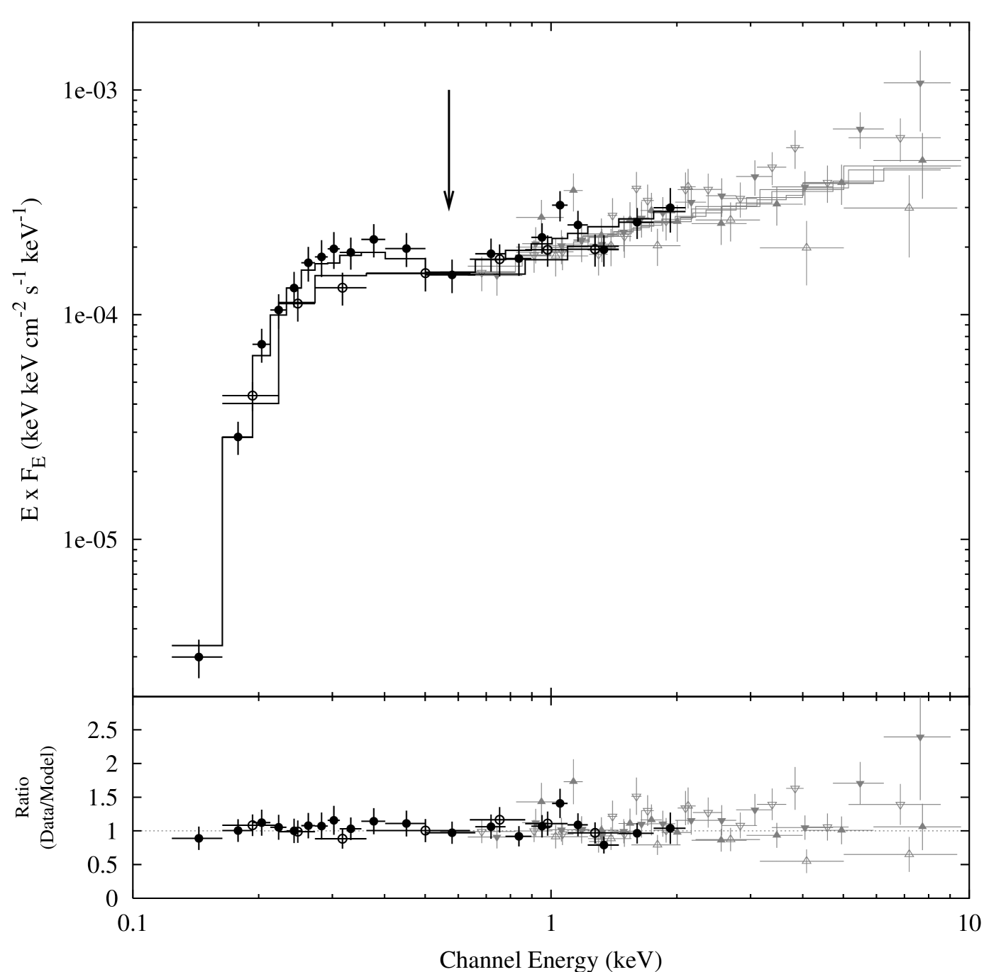
Confidence contours for the best-fit model for the two parameters of interest, equivalent Hydrogen absorbing column () and the spectral break energy, are shown in Fig. 2. The soft x-ray absorption at cm-2 is above the Galactic level of cm-2 given by Dickey & Lockman Dickey & Lockman (1990).

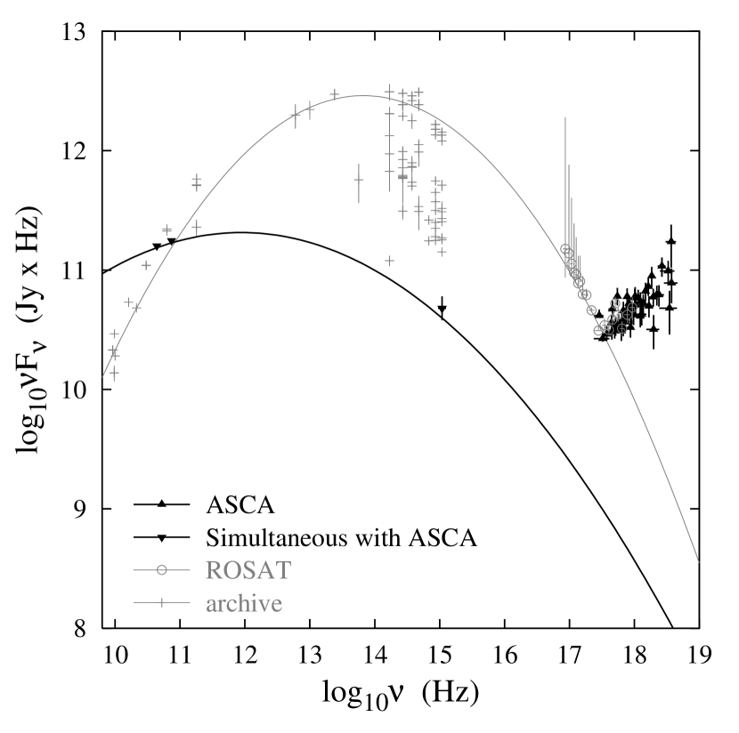
The rest-frame SED is plotted in Fig. 1. The break in the ROSAT spectrum is clearly evident at 1.1 keV ( Hz). It is generally accepted that the two broad emission components that characterise blazar SEDs are due to synchrotron emission at lower energies and inverse Compton (IC) emission at higher energies Costamante et al. (2000); Fossati et al. (2000); Sambruna et al. (1996); Pian et al. (1996) The SED of B2 1308+326 shows the synchrotron component peaking between Hz and Hz with the inverse Compton emission dominating by Hz. The parabolic fit to the contemporaneous data indicates that the peak synchrotron frequency is Hz (Fig. 1). Although no variation in the 0.5–2.4 keV spectra was detected between the observations made with ROSAT and ASCA, examining the SED (Fig. 1) leads to the conclusion that the ROSAT synchrotron flux is incompatible with the radio and optical data obtained contemporaneously with ASCA. The effect of the absence of the synchrotron flux on the R1 spectrum was quantified by extrapolating the best-fit ROSAT synchrotron power-law past the spectral break to 2.4 keV. The 0.5–2.4 keV flux of this synchrotron power-law alone was subtracted from the composite synchrotron-IC R1 0.5–2.4 keV flux. The resulting (IC) flux was still fully consistent with the ASCA 0.5–2.4 keV flux. This indicates that the synchrotron-IC break occurred at lower energies during the ASCA observation than during R1 and that the ASCA spectrum is almost entirely dominated by an IC component that has not varied substantially at these energies despite the large change in the synchrotron flux. Chiaberge & Ghisellini Chiaberge & Ghisellini (1999) have modelled synchrotron–self-Compton emission in blazars and successfully reproduced the SED of Mkn 421 in different flux states Macomb et al. (1995). Their model allows a peak synchrotron variation of nearly two orders of magnitude that leaves the low-frequency end of the IC component largely unaffected, consistent with the SED observed here and in Mkn 421 Macomb et al. (1995). Major variability of the IC component would however be expected at -ray energies because of the large change in the synchrotron emission. Observations at -ray energies can strongly constrain synchrotron-IC models Maraschi et al. (1999). A parabolic fit to the highest archival fluxes in each waveband and the ROSAT data below the spectral break yields a peak synchrotron frequency of Hz. This indicates that the peak synchrotron frequency of B2 1308+326 may decrease with flux, an important indicator in deciding the nature of the inverse Compton emission in this source Böttcher (1999). This type of spectral break and the possibility of increasing synchrotron peak frequency with increasing flux have also been observed with BeppoSAX in the blazar S5 0716+714 Giommi et al. (1999).
The ASCA lightcurve yields no evidence for variability above erg cm-2 s-1 on timescales of hours. V-band optical photometry from both Calar Alto observations yields a magnitude of . A limit on the variability of the source of 0.08 mag. was found using differential photometry. Therefore, no constraints can be placed on the superluminal gravitational lensing scenario in this AGN because of the absence of variability.
The optical spectrum (Fig. 4) observed on 16 June 1996 is intermediate between the extreme spectra previously observed Miller et al. (1978); Stickel et al. (1993).

The equivalent width of the Mg ii line was 15 Å. The absolute flux calibration for this spectrum is unreliable due to non-photometric conditions during the observation; it was therefore not possible to obtain a continuum level or line fluxes from the ASCA observations.
The results of the radio observations (Fig. 5) over 20 years indicate that B2 1308+326 was in an intermediate radio flux state during these observations.

5 Discussion
Although BL Lacs were originally classified as XBLs or RBLs depending on the energy band in which they were first discovered, recent work has focused on determining the physical distinctions between the two types Padovani & Giommi (1995); Fossati et al. (1997); Georganopoulos & Marscher (1998b) and their relation to the other subclass of blazar, FSRQs Sambruna et al. (2000); Sambruna (1997); Fossati et al. (1998); Ghisellini et al. (1998). The spectral energy distributions of XBLs and RBLs differ markedly, with the peak in synchrotron output generally occurring in the x-ray range for the former and the infrared range for the latter Padovani & Giommi (1995). This property has allowed BL Lacs to be classified as low-frequency peaked BL Lacs (LBLs, roughly the same sample as RBLs) and high-frequency peaked BL Lacs (HBLs, approximate to XBLs). Such differences may arise due to changes in the dominant radiation mechanism occurring as a function of both the angle between the line of sight and the bulk velocity Ghisellini & Maraschi (1989), although it has been demonstrated, assuming certain conditions, that the complete range of properties observed in blazars are difficult to account for solely by a change in orientation of the jet Sambruna et al. (1996). On the other hand, XBLs and RBLs have different variability timescales, a fact that is very naturally explained with the orientation hypothesis Heidt & Wagner (1998). The recent RGB sample revealed BL Lacs intermediate between XBLs and RBLs, indicating that there is no bi-modal distribution in BL Lacs and that they span peak synchrotron frequencies continuously from IR to x-ray wavelengths Laurent-Muehleisen et al. (1999).
One hypothesis connecting FSRQs and BL Lacs is that they are high and low luminosity radio galaxies respectively that are highly-relativistically beamed towards the observer Padovani (1992). A more recent theory connects FSRQs, LBLs and HBLs in a sequence of increasing peak synchrotron frequencies and decreasing bolometric luminosity Fossati et al. (1998); Sambruna et al. (2000); however, roughly 25% of FSRQs in the Deep X-ray Radio Blazar Survey Perlman et al. (1998) have HBL-like radio–x-ray broadband spectral indices (), indicating that the synchrotron peak frequencies () for FSRQs reach energies at least as high as those of HBLs, since is strongly correlated with (Fossati et al., 1998, and references therein). In this theory, blazars with strong thermal emission or strong emission lines (FSRQs) should have soft x-ray spectra dominated by inverse Compton (IC) emission produced by jet electrons scattering photons produced externally to the jet (external Compton, EC model). Blazars with intrinsically weak emission lines (BL Lacs) are expected to have their IC component dominated by jet electrons scattering photons produced in the jet via synchrotron emission (synchrotron self-Compton, SSC model). Böttcher Böttcher (1999) has postulated that EC-dominated spectra have peak synchrotron frequencies that decrease with increases in flux. The peak synchrotron frequency of B2 1308+326 appears to decrease with decreasing flux. While this synchrotron peak shift behaviour is contrary to the trend found in samples of blazars Kubo et al. (1998); Fossati et al. (1998) it is not at all unusual in flares detected in individual sources (e.g. Catanese et al. 1997). Without IR photometry it is not possible to determine precisely the peak synchrotron frequency at the time of these observations. The optical observations were obtained simultaneous with, and two weeks after, the ASCA observations and yielded compatible results on both occasions. The radio data nearest the ASCA observations were taken on 4 June 1996 at 37 GHz, and on 5 and 20 June 1996 at 22 GHz. The radio variability during the surrounding months was less than 30%. The spectrum would have to deviate significantly from a parabolic shape in order to peak above Hz and still manage to drop as low as 18.3 mag. in the optical. Such a spectral shape cannot be ruled out without accurate modelling of the synchrotron component, however it is very likely that the synchrotron peak did occur below Hz in the faint state observed here, indicating that the synchrotron peak frequency decreases with decreasing flux and that SSC is the more likely emission mechanism in this blazar Böttcher (1999). Simultaneous GeV observations are required to determine if there is excess IC emission resulting from the EC component. Such observations would be useful for testing the model proposed for PKS 0548+134 Mukherjee et al. (1999) and the trend detected by Kubo et al. Kubo et al. (1998) in a sample of 18 blazars.
The dominance of the IC component in B2 1308+326 above Hz is evident from Fig. 1. The relatively low energy of this break is consistent with expectations of LBLs Giommi et al. (1995), but somewhat exceeds expectations for FSRQs in the blazar paradigm described by Sambruna et al. Sambruna et al. (2000). The contemporaneous nature of the observations rules out distortion of the spectrum due to source variability.
The primary reason for classifying B2 1308+326 as a BL Lac rather than a FSRQ is its largely featureless optical continuum which is one of the defining features of the BL Lac class, with rest-frame W Å for any line Sambruna et al. (1996). This criterion has been justifiably criticised as arbitrary Kollgaard et al. (1992); Marchã et al. (1996); Scarpa & Falomo (1997) partly on the basis that some sources (such as B2 1308+326) have Wλ that vary substantially across this boundary. Nevertheless, weak or absent emission lines is a distinguishing property of these sources Padovani (1992). The rest-frame Wλ of the Mg ii line in B2 1308+326 detected by Miller et al. Miller et al. (1978) was Å and no lines were observed by Wills & Wills Wills & Wills (1979). However, an Mg ii W Å in the rest-frame was observed in March 1989 by Stickel et al. Stickel et al. (1993) in a very low luminosity state m mag (AB mag from the spectrum), comparable in brightness to the observations presented here. The Wλ ( Å) reported in this paper and by Stickel et al. Stickel et al. (1993) place B2 1308+326 outside the traditional limits for BL Lacs, while previous observations place it well inside.
The level of the continuum may be the most significant factor in changing the value of Wλ for the Mg ii line and not variation of the intrinsic line luminosity, since (a) both large Wλ measurements were made near low luminosity states and (b) the line flux of erg cm-2 s-1 reported by Miller et al. Miller et al. (1978) is within a factor of two of the value of erg cm-2 s-1 of Stickel et al. Stickel et al. (1993) even though Wλ differs substantially between the observations. No error was given for these measurements. Padovani Padovani (1992) has shown that in general the low values of Wλ observed in BL Lacs are due to intrinsically less luminous line fluxes than in quasars. Sambruna et al. Sambruna et al. (2000) find Mg ii luminosities of L(4–40) erg s-1 for a sample of three FSRQs, comparable to but higher than B2 1308+326, with L erg s-1. It therefore appears that the small values of Wλ observed in B2 1308+326 are due mostly to the extremely bright continuum. Unfortunately, it was not possible to obtain a line flux from these observations. Similar intermediate BL Lac–QSO behaviour is not unique to B2 1308+326, and has also been observed in PKS 0521-365 for example Scarpa et al. (1999).
The existence of sources intermediate between BL Lac and QSOs is expected in the blazar unification paradigm presented by Fossati et al. Fossati et al. (1998), where synchrotron peak frequency is correlated with source luminosity. X-ray, optical and radio luminosities for B2 1308+326 are compared to averages for the different blazar samples examined by Fossati et al. Fossati et al. (1998) in Table 4. It is interesting to note that the luminosities for B2 1308+326 span the range between the RBL-FSRQ averages.
| Band | XBLs (Slew) | RBLs (1 Jy) | FSRQ | B2 1308+326 |
|---|---|---|---|---|
| 5 GHz | 41.71 | 43.69 | 44.81 | 45.4 (44.0) |
| V-band | 44.91 | 45.68 | 46.58 | 45.1 (46.7) |
| 1 keV | 44.94 | 44.72 | 45.98 | 44.9 |
Sources intermediate between BL Lac and QSOs with luminous emission lines that are SSC-dominated and have high synchrotron peak frequencies Perlman et al. (1998); Sambruna et al. (2000) still pose serious problems to the unification scheme proposed by Fossati et al. Fossati et al. (1998). It has recently been pointed out Georganopoulos (2000) that the observed differences between FSRQs with high synchrotron peak frequencies (“blue quasars”) and HBLs can be explained by taking into account the orientation of the jet as well as the intrinsic source luminosity. In a similar way earlier unification schemes have attempted to unify intrinsically lower luminosity FR I radio galaxies with BL Lacs and the higher luminosity FR II radio galaxies with quasars Padovani (1992); Ghisellini et al. (1993). It now seems likely that quasars and BL Lacs form two distinct populations of higher and lower luminosity AGN respectively, where the orientation of the jet influences the luminosity and peak synchrotron frequency. The unusual intermediate properties of B2 1308+326 make it an ideal candidate for studying the overlap between the BL Lac and QSO categories. It may therefore represent the prototype of this kind of composite source.
5.1 Gravitational microlensing
The gravitational microlensing scenario Gabuzda et al. (1993); McBreen & Metcalfe (1987), provides an alternate explanation for the BL Lac properties of B2 1308+326. Its high bolometric luminosity is comparable to that of other gravitationally lensed candidates AO 0235+164 Rabbette et al. (1996) and PKS 0537-441 Romero et al. (1999); Perlman et al. (1996) and may be due to amplification by a foreground galaxy. Mg ii absorption lines with very small Wλ ( Å) were reported Miller et al. (1978) at in B2 1308+326. These lines have not been confirmed by later observations. Recent imaging with HST Urry et al. (1999) did not confirm the detection of spatially extended emission Stickel et al. (1993) and no evidence was found for a foreground lensing galaxy. Such a galaxy is therefore limited to an I-band magnitude greater than 20.1, which, if the galaxy were at a redshift implies M, thus not constraining its luminosity significantly. The absorbing column towards B2 1308+326 is greater than that expected from our Galaxy (Fig. 2). The excess absorption could be due to an absorber at or equally, to absorption in the host galaxy of B2 1308+326. The detection of excess absorption therefore does not exclude the possibility of a foreground lensing galaxy. A more detailed spectroscopic observation with XMM could determine the redshift of the foreground absorber. Sensitive, high-resolution optical spectroscopy could confirm the detection of Mg ii absorption lines Miller et al. (1978) and thus also determine the redshift of such an absorber.
5.2 Constraints on beaming in B2 1308+326
| TB | ||||||||||||
|---|---|---|---|---|---|---|---|---|---|---|---|---|
| (Jy) | (GHz) | (Jy) | (keV) | (GHz) | (mas) | ( K) | () | |||||
| 1.97Gh | 5.0Gh | Gh | 1Gh | Gh | 0.75Gh | 15.75 | 0.5Gh | 0.996Gh | 6.8Gh | 1.11Gh | 6.1 | 21.7 |
| – | – | – | – | – | – | 15.75 | – | 0.992T | 1.9T | 6.40T | 7.2 | 68.0 |
| 1.22Ga | 5.0Ga | 0.80 | 15.75 | 0.05Ga | 0.997 | 122 | 69.0 | 0.12 | 62.0 | |||
| 0.76Ga | 5.0Ga | 0.80 | 15.75 | 0.18Ga | 0.997 | 9.4 | 3.35 | 5.37 | 18.0 |
Contemporaneous multiwavelength observations allow the determination of a lower limit on the doppler boost factor (), the corresponding observed brightness temperature TB, the maximum angle () between the line of sight and the velocity of the relativistic jet as well as the minimum Lorentz factor of the jet, . Ghisellini et al. Ghisellini et al. (1993) have derived these values for B2 1308+326 with data from different epochs, using the equations:
| (1) |
| (2) |
| (3) |
and
| (4) |
where and are the fluxes in Jy at the synchrotron self-absorption frequency, (GHz), and at the x-ray or optical energy, (keV) respectively; is the synchrotron high energy cut-off frequency; is the spectral index of the thin synchrotron emission defined from ; is the fastest reported apparent superluminal speed; is the VLBI FWHM core size Marscher (1977) in milliarcseconds (mas) at ; is the redshift of the source. A comparison of these values obtained at different epochs for b2 1308+326 is made in Table 5.
It has been noted that the largest source of error in Eq. (1) is the determination of the VLBI core size, Madau et al. (1987). This value is crucial in determining the limit on .
Ghisellini et al. Ghisellini et al. (1993) calculate using mas at 5 GHz. High resolution VLBI images of B2 1308+326 were presented by Gabuzda et al. Gabuzda et al. (1993) obtained in 1987 and 1989. Using the 5 GHz fluxes and corresponding FWHM core sizes of Gabuzda et al. Gabuzda et al. (1993), values of and were determined with the data presented here. Clearly the core size is variable and further constraints on would require VLBI imaging simultaneous with observations at other wavelengths.
Teräsranta & Valtaoja Teräsranta & Valtaoja (1994) use the radio variability timescales of B2 1308+326 to deduce a lower limit for the doppler boost factor of and the corresponding maximum observed brightness temperature T K. The 22 GHz light curve used for this calculation is plotted in Fig. 5. This method provides a useful independent measure of . A comparison of these values with those derived using Eqs. (1)–(4) are given in Table 5. Two sets of values have been derived with the data obtained contemporaneously with ASCA using the different core sizes reported by Gabuzda et al. Gabuzda et al. (1993). The contemporaneous data indicates that the synchrotron peak frequency is roughly Hz (Fig. 1) and this value was used for . A similar fit to the highest archival fluxes in each waveband and the ROSAT data below the spectral break yields a peak synchrotron frequency of Hz. The V-band flux and frequency were used instead of the 1 keV flux in these calculations, as the 1 keV flux at the time of these observations was almost certainly dominated by inverse Compton emission.
Three of the limits on agree within a factor of five (Table 5). The extreme value of , obtained using the core size mas, is unlikely given the low flux state of the source during these observations. While the upper limits on are consistent with expected jet angles for RBLs, they are also consistent with those of highly-polarised quasars (HPQs; Ghisellini et al. 1993, Urry & Padovani 1995). Quasars generally appear to have larger values of than BL Lacs Gabuzda et al. (1993); Teräsranta & Valtaoja (1994). A mean of 8.3 for HPQs and 1.3 for BL Lacs Gabuzda et al. (1993) indicates that B2 1308+326 with , is rather extreme for a typical BL Lac.
6 Conclusions
The blazar B2 1308+326 was observed contemporaneously at x-ray, optical and radio wavelengths in June 1996. The source was in a low synchrotron flux state at the time of observation and no variability was detected. The ROSAT data reveal an x-ray spectrum that is best fit by a broken power law with absorber model, with the break at keV in the rest-frame of the blazar. The break is probably due to the emerging dominance of the IC over the synchrotron component. The frequency of the peak synchrotron emission component appears to have decreased with decreasing flux, thus indicating that SSC may be the dominant emission mechanism in this source. The x-ray IC component is unaffected by the large change in the synchrotron emission. Mg ii emission was observed with rest W 15Å, significantly different from the Wλ values previously reported. The variable Wλ emission in B2 1308+326 is probably mostly due to the highly variable continuum. Although values of Wλ are quite small, the line luminosity is only slightly lower than in a sample of QHBs. A lower limit on the Doppler boost factor obtained from the contemporaneous data is consistent with expectations for HPQs but is higher than expected for BL Lacs. X-ray absorption at a level in excess of the Galactic value was detected and indicates the possible presence of a foreground absorber.
B2 1308+326 is a typical RBL in terms of peak synchrotron power and optical variability, but with a very large bolometric luminosity, variable line emission and a high Doppler boost factor also has quasar-like attributes. It may be an intermediate or transitional AGN or a gravitationally microlensed quasar, given its absorption above the Galactic level. Future x-ray observations could determine the nature of the absorber. Further simultaneous multiwavelength observations of this possibly prototypical intermediate blazar could determine the cause of both its BL Lac and its quasar-like properties, providing insight into the relation between BL Lacs and FSRQs.
Acknowledgement.
We would like to thank A. Celotti, for helpful comments that resulted in significant improvements to the paper.
References
- Angel & Stockman (1980) Angel J. R. P., Stockman H. S., 1980, ARA&A 18, 321
- Bevington & Robinson (1992) Bevington P. R., Robinson D. K., 1992, In: Data reduction and error analysis for the physical sciences, 2nd ed., McGraw-Hill, New York
- Böttcher (1999) Böttcher M., 1999, ApJ 515, L21
- Brown et al. (1989) Brown L. M. J., Robson E. I., Gear W. K. et al., 1989, ApJ 340, 129
- Catanese et al. (1997) Catanese M., Bradbury S. M., Breslin A. C. et al., 1997, ApJ 487, L143
- Chiaberge & Ghisellini (1999) Chiaberge M., Ghisellini G., 1999, MNRAS 306, 551
- Comastri et al. (1995) Comastri A., Molendi S., Ghisellini G., 1995, MNRAS 277, 297
- Costamante et al. (2000) Costamante L., Ghisellini G., Giommi P. et al., 2000, astro-ph/0001410
- Dickey & Lockman (1990) Dickey J. M., Lockman F. J., 1990, ARA&A 28, 215
- Fanaroff & Riley (1974) Fanaroff B. L., Riley J. M., 1974, MNRAS 167, 31p
- Fiorucci et al. (1998) Fiorucci M., Tosti G., Rizzi N., 1998, PASP 110, 105
- Fossati et al. (1997) Fossati G., Celotti A., Ghisellini G., Maraschi L., 1997, MNRAS 289, 136
- Fossati et al. (1998) Fossati G., Maraschi L., Celotti A., Comastri A., Ghisellini G., 1998, MNRAS 299, 433
- Fossati et al. (2000) Fossati G., Celotti A., Chiaberge M. et al., 2000, astro-ph/0005066
- Gabuzda et al. (1993) Gabuzda D. C., Kollgaard R. I., Roberts D. H., Wardle J. F. C., 1993, ApJ 410, 39
- Georganopoulos (2000) Georganopoulos M., 2000, astro-ph/0008482
- Georganopoulos & Marscher (1998a) Georganopoulos M., Marscher A. P., 1998a, ApJ 506, L11
- Georganopoulos & Marscher (1998b) Georganopoulos M., Marscher A. P., 1998b, ApJ 506, 621
- Ghisellini & Maraschi (1989) Ghisellini G., Maraschi L., 1989, ApJ 340, 181
- Ghisellini et al. (1993) Ghisellini G., Padovani P., Celotti A., Maraschi L., 1993, ApJ 407, 65
- Ghisellini et al. (1998) Ghisellini G., Celotti A., Fossati G., Maraschi L., Comastri A., 1998, MNRAS 301, 451
- Giommi et al. (1995) Giommi P., Ansari S. G., Micol A., 1995, A&AS 109, 267
- Giommi et al. (1999) Giommi P., Massaro E., Chiappetti L. et al., 1999, A&A 351, 59
- Gopal-Krishna & Subramanian (1991) Gopal-Krishna, Subramanian K., 1991, Nat 349, 766
- Heidt & Wagner (1998) Heidt J., Wagner S. J., 1998, A&A 329, 853
- Inoue (1993) Inoue H., 1993, Experimental Astronomy (ISSN 0922-6435) 4, 1
- Iwasawa et al. (1999) Iwasawa K., Fabian A. C., Nandra K., 1999, MNRAS 307, 611
- Kollgaard et al. (1990) Kollgaard R. I., Wardle J. F. C., Roberts D. H., 1990, AJ 100, 1057
- Kollgaard et al. (1992) Kollgaard R. I., Wardle J. F. C., Roberts D. H., Gabuzda D. C., 1992, AJ 104, 1687
- Kollgaard et al. (1996) Kollgaard R. I., Gabuzda D. C., Feigelson E. D., 1996, ApJ 460, 174
- Kubo et al. (1998) Kubo H., Takahashi T., Madejski G. et al., 1998, ApJ 504, 693
- Lamer et al. (1996) Lamer G., Brunner H., Staubert R., 1996, A&A 311, 384
- Laurent-Muehleisen et al. (1999) Laurent-Muehleisen S. A., Kollgaard R. I., Feigelson E. D., Brinkmann W., Siebert J., 1999, ApJ 525, 127
- Macomb et al. (1995) Macomb D. J., Akerlof C. W., Aller H. D. et al., 1995, ApJ 449, L99
- Madau et al. (1987) Madau P., Ghisellini G., Persic M., 1987, MNRAS 224, 257
- Maraschi et al. (1999) Maraschi L., Fossati G., Tavecchio F. et al., 1999, ApJ 526, L81
- Marchã et al. (1996) Marchã M. J. M., Browne I. W. A., Impey C. D., Smith P. S., 1996, MNRAS 281, 425
- Marscher (1977) Marscher A. P., 1977, ApJ 216, 244
- McBreen & Metcalfe (1987) McBreen B., Metcalfe L., 1987, Nat 330, 348
- Miller et al. (1978) Miller J. S., French H. B., Hawley S. A., 1978, In: A. M. Wolfe (ed.), Pittsburgh Conference on BL Lac Objects, pp 176–191, University of Pittsburgh, Pittsburgh
- Morrison & McCammon (1983) Morrison R., McCammon D., 1983, ApJ 270, 119
- Mufson et al. (1985) Mufson S. L., Stein W. A., Wisniewski W. Z. et al., 1985, ApJ 288, 718
- Mukherjee et al. (1999) Mukherjee R., Böttcher M., Hartman R. C. et al., 1999, ApJ 527, 132
- Nottale (1986) Nottale L., 1986, A&A 157, 383
- Ostriker & Vietri (1990) Ostriker J. P., Vietri M., 1990, Nat 344, 45
- Padovani (1992) Padovani P., 1992, MNRAS 257, 404
- Padovani & Giommi (1995) Padovani P., Giommi P., 1995, ApJ 444, 567
- Perlman et al. (1996) Perlman E. S., Stocke J. T., Schachter J. F. et al., 1996, ApJS 104, 251
- Perlman et al. (1998) Perlman E. S., Padovani P., Giommi P. et al., 1998, AJ 115, 1253
- Pfeffermann & Briel (1986) Pfeffermann E., Briel U. G., 1986, Proceedings of SPIE 597, 208
- Pian et al. (1996) Pian E., Falomo R., Ghisellini G. et al., 1996, ApJ 459, 169
- Pian et al. (1998) Pian E., Vacanti G., Tagliaferri G. et al., 1998, ApJ 492, L17
- Rabbette et al. (1996) Rabbette M., McBreen B., Steel S., Smith N., 1996, A&A 310, 1
- Rabbette et al. (1998) Rabbette M., McBreen B., Smith N., Steel S., 1998, A&AS 129, 445
- Romero et al. (1999) Romero G. E., Cellone S. A., Combi J. A., 1999, A&AS 135, 477
- Sambruna (1997) Sambruna R. M., 1997, ApJ 487, 536
- Sambruna et al. (1996) Sambruna R. M., Maraschi L., Urry C. M., 1996, ApJ 463, 444
- Sambruna et al. (1999) Sambruna R. M., Ghisellini G., Hooper E. et al., 1999, ApJ 515, 140
- Sambruna et al. (2000) Sambruna R. M., Chou L. L., Urry C. M., 2000, ApJ 533, 650
- Scarpa & Falomo (1997) Scarpa R., Falomo R., 1997, A&A 325, 109
- Scarpa et al. (1999) Scarpa R., Urry C. M., Falomo R., Treves A., 1999, ApJ 526, 643
- Stickel et al. (1991) Stickel M., Fried J. W., Kühr H., Padovani P., Urry C. M., 1991, ApJ 374, 431
- Stickel et al. (1993) Stickel M., Fried J. W., Kühr H., 1993, A&AS 98, 393
- Tanaka et al. (1994) Tanaka Y., Inoue H., Holt S. S., 1994, PASJ 46, L37
- Teräsranta & Valtaoja (1994) Teräsranta H., Valtaoja E., 1994, A&A 283, 51
- Teräsranta et al. (1998) Teräsranta H., Tornikoski M., Mujunen A. et al., 1998, A&AS 132, 305
- Urry & Padovani (1995) Urry C. M., Padovani P., 1995, PASP 107, 803
- Urry et al. (1999) Urry C. M., Falomo R., Scarpa R. et al., 1999, ApJ 512, 88
- Urry et al. (2000) Urry C. M., Scarpa R., O’Dowd M. et al., 2000, ApJ 532, 816
- Watson et al. (1999) Watson D., Hanlon L., McBreen B. et al., 1999, A&A 345, 414
- Wills & Wills (1979) Wills B. J., Wills D., 1979, ApJ 41, 689