Steady-state conduction-driven temperature profile in clusters of galaxies

Abstract

The temperature profile (TP) of the intracluster medium (ICM) is of primeval importance for deriving the dynamical parameters of the largest equilibrium systems known in the universe, in particular their total mass profile. Analytical models of the ICM often assume that the ICM is isothermal or parametrize the TP with a polytropic index $\gamma_{p}$. This parameter is ajusted to observations, but has in fact poor physical meaning for values other than 1 or 5/3, when considering monoatomic gases. In this article, I present a theoretical model of a relaxed cluster where the TP is instead structured by electronic thermal conduction. Neglecting cooling and heating terms, the stationnary energy conservation equation reduces to a second order differential equation, whose resolution requires two boundary conditions, taken here as the inner radius and the ratio between inner and outer temperature. Once these two constants are chosen, the TP has a fixed analytical expression, which reproduces nicely the observed “universal” TP obtained by Markevitch et al. (1998) from ASCA data. Using observed X-ray surface brightnesses for two hot clusters with spatially resolved TP, the local polytropic index and the hot gas fraction profile are predicted and compare very well with ASCA observations (Markevitch et al 1999). Moreover, the total density profile derived from observed X-ray surface brightness, hydrostatic equilibrium and the conduction-driven TP is very well fit by three analytical profiles found to describe the structure of galactic or cluster halos in numerical simulations of collisionless matter (Hernquist, 1991; Navarro et al. 1995, 1997; Burkert 1995).

The suppression of the heat conduction several orders of magnitude below the Spitzer rate is an important assumption of the cooling-flow models, in order to ensure the thermal instability ability to trigger further condensation and cooling of density perturbations, although no definitive theoretical picture of this reduction has yet been put forward. In consequence, electronic heat conduction has seldom been considered for the structure of the main volume of the cluster, outside the cooling flow radius. However, the physical situation outside the cooling flow differs widely from the one inside, the temperature gradient being much shallower, the magnetic field intensity much smaller (as shown by the Faraday rotation measures and predicted by Soker & Sarazin, 1990) and the cooling time higher than the mean age of the structure. Thus, it is not obvious that the mechanism reducing the heat flux in the cooling flow is as highly effective in the main body of a cluster. If the TP decline in clusters is confirmed by the new generation of X-ray telescopes (Chandra and XMM-Newton), this simple conduction-driven model of the cluster ICM equilibrium could give useful insights on the physical situation in this region and the predicted shape of the TP (related to the temperature dependance of the heat flux for a collisionally-ionised plasma) will be tested directly against observations.

1 Introduction

The numerical simulations of the formation of clusters in a realistic cosmological frame seem to have reached a fair state, since the first runs of two-fluid P3MSPH simulations by Evrard (1988, 1990). Recently, Frenk et al. (1999) have compared, using 12 different codes, the final output of the simulation of an X-ray cluster in a CDM universe, and have found that the overall agreement is impressive, except for quantities requiring an enhanced resolution, such as the total X-ray luminosity. Moreover, although agreement does not guarantee correctness (as scaling law models can only give the evolution of an ideal population of standard clusters), the results of simulations are remarkably fitted by predictions of approximate analytic models (Navarro, Frenk & White 1995 hereafter NFW95, Eke, Navarro & Frenk 1998, Bryan & Norman 1998). Thus, it seems that numerical simulations of clusters are a reliable implementation of the physical processes invoked for the adiabatic formation of clusters.

However, these simulations make the simplifying assumption that only gravity, pressure gradients and hydrodynamical shocks are important in the evolution of clusters. Moreover, when the results of observed statistical properties of X-ray clusters are compared to simulations, one of the most basic observed relations, namely the $L_{X}-T$ relation, cannot be reproduced, being shallower than the observations (see Bryan & Norman, 1998). This relation is of fundamental importance since it links the mean temperature (thought as imposed by the total mass) and the luminosity (which goes as the baryonic density squared times the cube of a characteristic radius of the X-ray halo). Thus, the $L_{X}-T$ relation shows the changes with temperature in the equilibrium state of the baryonic gas in the underlying dark matter potential. The same flattening of the $L_{X}-T$ relation, which corresponds to a steepening of the luminosity function (as compared to observations) was found by Kaiser (1991) and Evrard & Henry (1991) in the validation of adiabatic scaling law models. Both found that an early preheating phase (maybe galactic feedback or quasar formation), enhancing the initial adiabat of the gas before cluster formation, could solve this problem, decreasing the final density and thus the final luminosity. Since low virial temperature systems are more sensitive to this phenomenon, the $L_{X}-T$ relation is steepened in the correct way. Such a scenario has been crudely incorporated in numerical simulations by assuming a higher initial temperature (Evrard 1990, NFW95) and effectively produces less dense clusters with larger X-ray core radii. Recently, such core X-ray properties of groups of galaxies as compared to clusters, have been interpreted as the presence of a minimum entropy threshold, higher than the only gravitational processes could have produced (Ponman, Cannon & Navarro 1998). Finally, semi-analytical models of structure formation, applied to groups and clusters of galaxies, have shown that an early injection by supernovae or quasars can reproduce the self-similarity breaking for structures with virial temperature smaller than $\sim 3\,\rm keV$ (see e.g. Cavaliere, Menci & Tozzi 1997,1998; Wu, Fabian & Nulsen 1999; Valageas & Silk 1999; Bower et al. 2000). Whatever the details of the equilibrium of the gas in the gravitational potential, this energy excess seems to be of the order of $\sim 1\,\rm keV$ per particle. Most of these models have considered that this energy was injected before the formation of clusters and groups but, considering the degeneracy between the redshift of injection and the value of the energy excess, late injection cannot be ruled out (see Loewenstein 2000).

It is interesting to note that not only the overall correlation of the cluster population between luminosity and temperature (or the number density of clusters at a fixed luminosity) are in disagreement with the observations , but also is the resulting structure of a single cluster evolved adiabatically until a relaxed state (see Evrard 1990, Chièze, Teyssier & Alimi 1998; the observed X-ray core radii are at least an order of magnitude larger than in the simulated cluster). This implies that preheating should not only affect the statistical correlations between clusters taken as a whole population, but also the internal structure of a particular forming cluster. After the turn-around, the number density of galaxies should be higher in the central part of a cluster than in the outer parts, producing a spatial gradient in the quantity of energy injected by galactic feedback, as well as in the metal content of the pre-cluster gas. This heating and enrichment can certainly have dramatic effects on the subsequent evolution of a parcel of gas, and are up-to-now only crudely approximated by numerical simulations (see e.g. Metzler & Evrard, 1994, NFW95). Thus, the relaxed temperature profile produced by numerical simulations could be significantly altered in a non-adiabatic model, producing, for example, a temperature gradient. In fact, recent ASCA spatially resolved cluster spectra (Markevitch et al 1998) and cluster hydrodynamics simulations (Frenk et al. 1999) seem to confirm a non-isothermal TP in relaxed clusters, even if ROSAT data may not show this gradient (Irwin, Bregman & Evrard 1999).

In this paper, I take the point of view that this non-isothermal TP is real and determine its spatial variation in a steady-state conduction-driven model. In the absence of a magnetic field, the electronic heat conduction should transport energy from hot inner gas to colder outer parts, thus strongly structuring the spatial behaviour of the temperature. In section 2, I write down the non-adiabatic energy conservation equation in this model and solve it for the temperature, before a comparison to X-ray observations and simulations of clusters. The next section uses the ROSAT X-ray brightness profile of A496 (Markevitch et al. 1999) to predict the local polytropic index and the hot gas fraction profile, which in turn are compared to ASCA spatially resolved data. Section 3 compares the total mass density profile resulting from hydrostatic equilibrium (hereafter HSE) hypothesis and the analytical TP derived before with analytic approximations derived from numerical simulations. Finally, section 4 discusses briefly the possible role of the magnetic field and the consequent inhibition of thermal conduction, to investigate the amount of time necessary to reach such a stationnary state.

Throughout the paper, whenever required, a Hubble constant of $H_{0}=50\,\rm km\,s^{-1}\,Mpc^{-1}$ is used.

2 Conduction-structured temperature profile in clusters

2.1 Assumptions

The mean free path of ions and electrons in the ICM are shorter than the scale length of interest in a cluster (Sarazin, 1988). Thus, the ICM will be described in the hydrodynamical approximation, and its evolution governed by the conservation of mass, momentum and energy. The collisionally ionized plasma is assumed single-phased and an ideal gas equation state is taken. Since we want to describe a relaxed state, a steady-state is assumed (i.e. all the terms involving a time derivative vanish). Moreover, hydrodynamical simulations have shown that the gas equilibrium is well described by HSE in the exterior dark matter potential $\phi$ within a radius $R_{500}$ defined by an interior density which is 500 times the mean density of the universe (Evrard, Metzler & Navarro 1996). In fact, for the sake of simplicity, we assume that the HSE holds until the virial radius of the cluster (defined as $R_{200}$ with obvious notations). Momentum conservation reduces then to the hydrostatic equation. All this modeling is done outside of the cooling flow radius, which is taken to be a fraction $x_{0}$ of the virial radius. We thus neglect the radiative cooling of the gas $\Lambda$. Finally, we also neglect the reheating term $\Gamma$ in the energy conservation equation. As highlighted in the introduction, this term cannot in general be neglected. But, since we describe the final state of equilibrium of a cluster, what we neglect is the present-day value of $\Gamma$, assuming nothing about the value it took before and during the collapse of the structure.

The thermal conduction flux is assumed to be given by the classical Spitzer rate (Spitzer, 1965) modified by an efficiency term $f$ ($0<f\leq 1$) to take into account a possible inhibition of the conduction (see Sec. 4), giving:

$${\bf q}=f\kappa_{0}T^{5/2}\nabla T,$$ (1)

where the logarithmic dependance of the Coulomb factor with the density has been ignored and $\kappa_{0}$ is a constant.

2.2 The energy equation for a non-isentropic conductive gas in hydrostatic equilibrium

Within these asumptions, the mass and energy conservation can be written:

$$\nabla.(\rho{\bf v})=0$$ (2)

$$\nabla.\left[\rho{\bf v}\left(\frac{v^{2}}{2}+h+\phi\right)-{\bf q}\right]=0$$ (3)

with $\phi$ the total gravitational potential, ${\bf v}$ the bulk velocity of the gas, $h$ its specific enthalpy and $\rho$ its density.

Assuming HSE means neglecting the spatial part of the lagangian derivative of the velocity $\left({\bf v}.\nabla\right){\bf v}$ , i.e. neglecting the terms which contain squares or higher orders of the velocity. Thus, equation (3) can be simplified to:

$$\nabla.\left[\rho{\bf v}\left(h+\phi\right)-{\bf q}\right]=0$$ (4)

Assuming spherical symmetry, the mass conservation can be integrated to give:

$$r^{2}\rho v=A_{0}.$$ (5)

where $A_{0}$ is an arbitrary constant and $v$ the radial velocity. We can integrate the energy conservation as well, and, using equation (5), we obtain ($C_{0}$ being another arbitrary constant):

$$A_{0}(h+\phi)-r^{2}\kappa_{0}T^{5/2}\frac{dT}{dr}=C_{0}$$ (6)

Since the gas is considered as perfect ($h=5kT/2$), equation (6) is a differential equation for the temperature, once the potential $\phi$ is fixed. The exact solution of this equation is beyond the scope of this paper, and we will restrict us to a special case which has an analytical solution. Suppose that the equilibrium is static, i.e. ${\bf v}={\bf 0}$. If we insert this condition in equation (3), we are left with:

$$\nabla.(\kappa(T)\nabla T)={\bf 0}.$$ (7)

In other words, the divergence of the heat flux due to conduction vanishes. This means that, apart from gravitation, there is no heat source or sink in the intracluster gas nowadays, since conduction is a transport process. If a temperature gradient is present, heat conduction freely transports energy from the inner hot parts to the outer colder parts. To compensate the energy loss of the center, an inflow of matter should appear which contracts the cluster, since the pressure gradient is still fixed by the hydrostatic condition (This idea is due to R. Teyssier). If this inflow is subsonic, the contraction will be adiabatic, thus the TP will still be structured by the local heat conduction and equation (9) should still be valid. The velocity profile induced and the computation of the exact loss of energy of the center are beyond the scope of this paper, which intends only to present the model and compare it to observations (see Dos Santos, 2000, in preparation)

In spherical symmetry, equation (7) can be written:

$$r^{2}f\kappa_{0}T^{5/2}\frac{dT}{dr}=C_{0}.$$ (8)

Once we have fixed two integration constants (two temperatures at two different radii, say the inner cooling radius and the virial radius), equation (8) can be integrated to give the TP. After some algebra, and rescaling the radius in units of the virial radius (i.e. $x=r/R_{200}$), we obtain:

$$\frac{T(x)}{T_{200}}=\left(1+(\eta^{7/2}-1)\frac{x_{0}}{x_{0}-1}\frac{x-1}{x}\right)^{2/7},$$ (9)

where $\eta=T_{0}/T_{200}$, $T_{0}$ being the inner temperature and $T_{200}$ the temperature at $r=R_{200}$. This analytic profile will be called hereafter Steady-State Conduction-Driven temperature profile (SSCD model).

Rephaeli (1977) already constructed a model where the TP was structured by electronic conduction. However, at this epoch, it was not clear whether the ICM was mostly primordial or composed by enriched gas ejected by galaxies. Thus, in his model, he assumed that the galaxies, today, inject gas in the ICM. This was done by adding a heating term to the heat transfer equation (eq.  7), which is proportional to the galaxy density profile, assumed to be a King profile and to be proportional to the total mass density profile. An analytic temperature profile is found, but depends on the assumed total mass profile. Here, on the contrary, I assume that $\Gamma(z=0)$ vanishes (see sec. 2.1), and thus don’t need to assume a total mass profile. The analytic temperature profile has a determined shape once two boundary conditions are set. On the other hand, using only X-ray observed quantities like the X-ray surface brightness profile (which was not yet known at the epoch of Rephaeli’s article), we can obtain the corresponding total mass profile (see section 3).

Finally, injecting the self-similar analytical form $T(x)/T_{200}=x^{\gamma}$ into equation 7, it is trivial to show that the only solutions have indexes $\gamma=-2/7$ or $0$ (the latter one corresponding to an isothermal cluster). The general solution differs from the self-similar one only near the virial radius, and reduces to it when $x_{0}=\eta^{-2/7}$.

We next compare the SSCD temperature profile obtained above with X-ray observations and outputs of numerical simulations.

2.3 Comparison to observations and simulations

Obtaining the TP of clusters of galaxies from X-ray spectroscopic and imaging data is not an easy task. ROSAT, with both PSPC detectors, was the first satellite to have enough spatial and spectral resolution to allow crude TPs to be obtained. Unfortunately, the spectral sensitivity of the detectors was negligible above $2.4\;{\rm keV}$, a temperature well below the mean temperature of rich clusters. Irwin et al. (1999) have searched without success for temperature gradients in ROSAT data of rich clusters. They did not derive the TP, but instead worked with hardness ratio profiles. However, because of its narrow energy band, ROSAT results are surely biased against the detection of a temperature decrease, especially if calibration uncertainties are not taken into account (Markevitch & Vikhlinin, 1997). However, using HEAO 1 A-2 and Einstein data without spatial resolution (but with different fields of view), Henriksen & White (1996) showed the need for a cold component to fit the spectral data in four clusters with cooling flows. The emission measure of this component was so large that it couldn’t be explained by the cooling flow component, and showed that large quantities of cold gas were lying outside the cooling flow, thus implying a declining TP (if the outer cold gas is in virial equilibrium in the cluster potential, which can not be infered from the spectroscopic data alone).

ASCA has much better spectral capabilities than ROSAT but the PSF correction is problematic. Nevertheless, a number of groups have published TPs for clusters. In particular, Markevitch et al. (1998, hereafter M98) found that 19 relaxed clusters (i.e. clusters with circular isophotes and without obvious substructure), when rescaled to their virial radius and to a flux-weighted mean temperature, had similar TPs within the error bars. The median TP declines outwards, the temperature decreasing by a factor of 2 within half the virial radius. It is not yet clear if these results are reliable because the PSF correction implies that the temperature measurements are correlated and the systematic effects are poorly known (see M98). Nevertheless, the next generation of X-ray satelites (Chandra, XMM, Astro-E) should probe the TP very soon. We will thus compare the SSCD temperature model to the M98 data.

Remark that the quasi self-similarity of the analytic solutions naturally explains the fact that all the clusters have the same temperature profile when rescaled to the virial radius, if the parameter $\eta$ is roughly constant in rich clusters (which is not proved here, but see Dos Santos 2000, in preparation). To compare properly the TP with M98’s observation, we must compute the emission-weighted TP, i.e.:

$$T_{ew}(R)=\frac{\int n_{g}^{2}(r)\Lambda[T(r)]T(r)ds}{\int n_{g}^{2}(r)\Lambda[T(r)]ds},$$ (10)

where the integrals are taken along the line-of-sight. To obtain the gas density $n_{g}(r)$, we assume that the surface brightness profile $\Sigma(R)$ is given by a standard $\beta-$model (Cavaliere & Fusco-Femiano 1976, 1978). This analytic form gives excellent fits outside of the cooling flow radius (Jones & Forman 1984). The two parameters of $\Sigma(R)$, namely the core radius and $\beta$ are fixed respectively to $R_{c}=0.1R_{200}$ and $\beta=2/3$. Those values are common in clusters and represent the “standard” cluster (Neumann & Arnaud 1999) used here. The gas density is obtained by an Abel inversion integral, with the cooling function being pure Brehmsstrahlung ($\Lambda(T)\sim T^{1/2}$), and then the emission-weighted TP is computed. The results are displayed in fig. 1. The same parameters are used for the computation of the total mass profile (sec. 3).

Figure 1: Comparison of the temperature profile with ASCA data of rich clusters. The dashed line is obtained with $\eta=3$ and $x_{0}=0.05$, while the dotted line with $\eta=5$ and $x_{0}=0.01$. The light-shaded band shows the $90\/\%$ error boundaries of the M98’s composite profile, while the dark shaded-band corresponds to a less conservative choice, approximating the scatter of the best-fit profile points.The solid line is the mass-weighted temperature profile obtained from averaging hydrodynamical simulations of the formation of a cluster (see text).

There is a very good agreement with the observations, even if the conductive profile seems to be less steep in the outer regions of the cluster. Remember that there are no data beyond half the virial radius, which means that the extrapolation is risky. However, interestingly, Markevitch et al. (1999) note that the TP for two clusters with high signal-to-noise data (A496 and A2199, which are not part of the sample of M98) is more concave, i.e. flatter in the outskirts , than their composite profile. They argue that this is a coincidence, but the model presented here explains naturally the flattening of the TP at large radius (see section 2.4).

Finally, the SSCD profile is compared to the mean temperature profile obtained by Frenk et al. (1999) from the average of twelve hydrodynamical simulations of the same cluster (solid line in figure 1). The virial radius was fixed to $R_{200}=2.7\,\rm Mpc$ and the mean temperature to $7\times 10^{7}\,\rm K$ (somewhat higher than the mass-weighted mean temperature to mimic emission-weighted mean temperature). The comparison is not obvious since the simulated TP is mass-weighted (using an emission-weighted TP would certainly steep the inner simulated profile), the hydrodynamical simulations are adiabatic, and thus no transport processes such as electronic thermal conduction are included and the simulated profile results from an average of 12 different simulations. The simulated cluster suffered its most recent strong merger at $z\sim 0.5$. During the phase of violent relaxation prevailing during a merger, large scale convection should be the main physical process through which energy is exchanged in the ICM. But, during the phase of relaxation, once the gravitational potential suffers no more large fluctuations, the heat conduction can play a significant local role in the establishment of the TP. Thus, the simulated temperature profile can be viewed as the initial TP on which the ETC will act to lead to the SSCD profile. Hence, perfect agreement between these two TPs is not expected. However, at a fixed central temperature, the gas internal energy in the center is higher in the simulated TP (keep in mind that mass-weighted and emission-weighted are here compared, which weakens the argument). The model described in sec. 2 (transfer by conduction of central energy followed by an adiabatic contraction) could easily lead to an SSCD profile, without changing much the central temperature (imposed by the central hydrostatic condition).

2.4 Local polytropic index

Mixing processes in the ICM, e.g. convection, are likely to make the specific entropy constant within the cluster, and thus lead to an adiabatic structure of the gas, where pressure and density are simply related by

$$s_{0}=c_{v}\ln\left(\frac{P}{\rho^{\gamma}}\right),$$ (11)

$s_{0}$ being the specific entropy (here considered as constant) and $c_{v}$ the specific heat at constant volume. If the gas is perfect, $\gamma$, the ratio of specific heat at constant pressure and volume ($\gamma=c_{p}/c_{v}$) is a constant and its value (always greater than 1) is fixed by the nature of the gas molecules : $5/3$ for a monoatomic gas, $7/5$ for a diatomic gas (see Landau & lifshitz 1959, p. 315). Even if the presence of metals in the ICM is spectroscopically important, in view of the considerable amount of lines they produce, it is safe to consider that the gas is mainly composed of monoatomic hydrogen, and thus that $\gamma=5/3$. This quantity should be kept constant throughout the ICM, since it depends on the nature of the plasma itself, and not on its dynamical behaviour.

The first non-isothermal models of the ICM were introduced by Lea (1975), Gull & Northover (1975) and Cavaliere & Fusco-femiano (1976). They assumed that the ICM was an isentropic perfect gas (with $\gamma=5/3$) in equilibrium in a static gravitational potential. They used equation (11), together with the equation of state of the gas, to close the hydrodynamics equations set and obtain the TP. The first two-fluid numerical simulations of cluster formation (Evrard 1990) have shown that the ICM is unlikely to be isentropic, due to the deepening of the potential well leading to a rising specific entropy profile with radius. Moreover, the first spatially resolved spectroscopy of clusters have also shown that these adiabatic models had TP which were too steep, compared to observations (Eyles et al. 1991, Markevitch et al. 1998). Thus, subsequent non-isothermal models have often used the following equation as a parameterization of the temperature profile, after obtention of the density profile via the HSE equation:

$$P\propto\rho^{\gamma_{p}}$$ (12)

In this approach, the polytropic index $\gamma_{p}$ is a parameter which is fitted to the spatially resolved spectroscopic data (see e.g. Cavaliere et al 1999, figure 5) or used in a two-parameter models family (Wu et al. 1999, figure 3; Loewenstein 2000). This parameter is no more related to the microscopic nature of the gas (this explains why it is called here $\gamma_{p}$ and not $\gamma$), and can span a range between 1 (isothermal model) and 5/3 (isentropic gas and upper limit of the convective stability, Scharzschild 1958). Despite the flexibility of this approach, it is little more than a mathematical expendiency and its main problem relies in that it links the TP to the gas density profile in an unphysical way: the density and the temperature are forced to track one another in an artificial way, which can lead to internal inconsistencies when applied to imaging and spectroscopic X-ray data (Hughes et al., 1988a,b). In the present work, on the contrary, the TP is derived from the resolution of the energy conservation equation, assuming the gas is perfect and has a constant ratio of the specific heats $\gamma=5/3$. Then, once the gravitational potential is fixed, this temperature solution can be inserted in the HSE equation, as in the papers cited above, to obtain the gas density profile, without adding another parameter. It is thus possible here to predict the local value of the parameter $\gamma_{p}$, via the equation (12). Here, $\gamma_{p}$ is not constant as a function of radius, but must still be lower than 5/3, in order to ensure convective stability of the cluster (which would erase any temperature gradient greater than the adiabatic gradient in some crossing times, and thus contradict the hypothesis of stationarity). For the sake of the comparison with TP observations, this method to predict $\gamma_{p}(r)$ (whose variation will then depend on the gravitational potential expression) will not be used here. Instead, we will use the surface brightness profile fitted to the X-ray data of a cluster to obtain the gas density profile, assuming that the X-ray photons are emitted via Brehmstrahlung and the TP is given by equation (9). The predicted local variations of $\gamma_{p}$ will be compared to the spatially resolved spectroscopic data of A496 from Markevitch et al. (1999, hereafter M99). The results are qualitatively the same with A2199, the second cluster whose data are also presented in the paper. The emission-weighted ASCA cooling-flow corrected temperature is $T_{X}=4.7\,\rm keV$, which gives a virial radius of $2.67\,\rm Mpc$, using the relation of Evrard et al. (1996). The surface brightness profile is taken from ROSAT PSPC data, and fitted (outside the cooling flow radius) with a $\beta-$model, giving a core radius of $249\,\rm kpc\equiv 0.093\times R_{vir}$ and a slope $\beta=0.7$. We use these values for the description of $S_{X}(R)$ and $(\eta,x_{0})=(3,0.05)$ for the TP (using $\eta=5$ and $x_{0}=0.01$ instead does not change appreciably $\gamma_{p}(r)$). Outside the cooling-flow radius, the TP is described well by a polytropic fit, with $\gamma_{p}=1.24^{+0.08}_{-0.11}$. The figure 2 shows the predicted $\gamma_{p}$ value (bold solid line), together with the best-fit value of M99 and its confidence interval (three horizontal lines, see caption). Despite the fact that no direct fitting of the TP has been made (the error bars on the data being still large, so we used the standard parameters of the TP used in section 2.3), the agreement with the constant polytropic index fitted value is impressive within the outer radius of the last ASCA data bin ($R_{max}\sim 1.3\,{\rm Mpc}\equiv 0.5\times R_{vir}$). Within this radius, the predicted $\gamma_{p}$ decreases from 1.25 in the center to 1.22 at 400 kpc, then increases again up to 1.36 at the virial radius. The value at $R_{max}$ is 1.26. $\gamma_{p}$ stays in the ASCA confidence interval up to $x=0.84$, but is always much smaller than the adiabatic gradient, which garanties convection stability within the virial radius. Note that M99 remark that the ASCA TP seems more concave than the polytropic fit (in fact, the observed TP is flatter than the fit in the outskirts). The same remark can be made when comparing A496 and A2199 data with the composite region from 19 clusters derived in M98. Interestingly, this is exactly what happens in the SSCD model: within $R_{max}$, the predicted value of $\gamma_{p}$, although being very close to the measured value, rises continously from 1.22 to 1.26, which flattens the TP, compared to a constant polytropic fit. Physically, it is easy to understand why this happens: the equation (7), when integrated over the surface of a sphere of radius r, stands that the total energy per unit time crossing the sphere surface is a constant, whatever the radius r (no source or sinks of energy are present in the ICM). The energy flux $q_{r}$, (i.e. the energy crossing a unit surface per unit time) will, on the other hand, depend on r as $q_{r}\propto r^{-2}$ in spherical symmetry. This flux will be much higher in the center (where the surface of the sphere is small, but the same amount of integrated energy crosses it) than in the outskirts. Since the flux is directly linked to the temperature gradient (equation 1), the TP will be much flatter in the outskirts than in the center. Even with ASCA, the error bars are still too large to allow a discrimination between the SSCD profile and a polytropic one, but the new generation of X-ray telescopes (XMM-Newton, Chandra) should be able to settle this case.

Figure 2: Predicted local polytropic index (bold solid line) compared to Abell 496 mean polytropic index ($\gamma_{p}=1.24^{+0.08}_{-0.11}$, light solid horizontal line and the two dashed horizontal lines). The maximum radius where ASCA spectroscopic data were available ($R_{max}\sim 1.3\,{\rm Mpc}\equiv 0.5\times R_{vir}$) is indicated by the vertical dashed-dotted line. $\eta=3$ and $x_{0}=0.05$ were used for this particular prediction, together with a $\beta-$model fit to the ROSAT PSPC surface brightness profile (see text).

2.5 hot gas fraction

If the gravitational instability picture of the formation of structures in the universe is crudely right, clusters of galaxies should be a fair sample of a patch of the early universe on a scale of $\sim 10\,\rm Mpc$. Thus, the amount of baryonic mass inside a cluster (hot diffuse gas as well as baryons locked into stars and interstellar medium in cluster galaxies) divided by the total mass should be also a fair sample of the baryonic fraction in the universe, since clusters are the largest structures in equilibrium so far discovered (if the dynamics of the formation are unable to expell baryonic material from the deep gravitational potential). This simple idea has been used as a cosmological test, mainly pointing to the fact that the measured gas fractions in clusters, if combined with a standard CDM universe, were incompatible with the big-bang nucleosynthesis results (White et al. 1993). The X-ray emissivity and the temperature profiles of the ICM, providing a direct lower limit on the baryonic fraction, are then a very useful tool to derive constraints on the value of the cosmological density parameter (see, for example, Ettori & Fabian 1999). Most of the recent observational work on X-ray clusters of galaxies has thus consisted in deriving the gas mass profile, in order to obtain a value for the gas mass fraction (hereafter GMF) at a fixed scaled radius (Evrard 1997; Arnaud & Evrard 1999; Mohr et al. 1999; Ettori & Fabian 1999; Vikhlinin, Forman & Jones 1999) for a large number of hot clusters (cool clusters or groups of galaxies being more sensitive to early energy injection and having a shallower potential well). These studies have shown so far that the gas mass profile seems to be similar in all clusters, when rescaled in proper units (Neumann & Arnaud 1999; Vikhlinin et al. 1999) and that, near the virial radius of these hot clusters, the GMF reaches a constant value, between $14$ and $20\,\%$ (the value depending mostly on the method and assumptions used to derive it, e.g. isothermal TP), which favours a low value of $\Omega_{0}$.

The derivation of the GMF profile is dependent on the TP, mostly because the total mass profile depends linearly on the TP. Proceeding like in the last section, it is then possible to compute the GMF profile: from the surface brightness profile and the SSCD model, the gas density profile is computed, which gives the gas mass profile after spatial integration. The total mass profile (assuming that the gas mass is negligible, which can be verified a posteriori) is derived from the HSE equation. The resulting GMF profile is compared to the A496 data in figure 3 (the data are represented by the shaded region, see figure 5 in M99). The predicted GMF has been normalised at the radius $R_{1000}$ (vertical dashed line at $x=0.37\equiv 1\,\rm Mpc$) at the value given by M99, i.e. 0.158.

The SSCD model predicts a TP which is unbounded in the center, thus the introduction of a minimum radius $x_{0}$ (physically identified with the cooling flow radius). The mass computation is then given by:

$$M_{gas}(x)=M_{gas}(x<x_{0})+m_{0}\int_{x_{0}}^{x}{x^{\prime}}^{2}\,\rho_{gas}(x^{\prime})\,dx^{\prime},$$ (13)

where, $M_{gas}(x)$ is the gas mass profile, $\rho_{gas}(x)$ is the gas density profile and $m_{0}$ is a constant. $M_{gas}(x<x_{0})$ is the mass interior to $x_{0}$, and is also a constant. The model can only give access to the value of the integral in the r.h.s.. If $M_{gas}(x<x_{0})$ is set to zero, we obtain the lowest curve on figure 3 (dash-dot line). Here, the gas mass is zero at $x=x_{0}$, and so is the GMF, which explains the deviation from the observations. Nevertheless, the prediction only crosses the boundary of the 90 $\%$ confidence interval for $x\lesssim 0.1$, and is consistent with the observations between $x=0.1$ and $x=0.37$ (0.267 and 1 Mpc respectively), but has a greater slope than them (it is not obvious how much of this effect is implied by the fact that M99 have used a polytropic TP to compute the mass profile, but this is probably negligible).

Instead, one can compute the integral in equation 13 with a minimum radius much less than $x_{0}=0.05$, say for example $x^{\prime}_{0}=x_{0}/100$ (values below this one don’t change much the GMF profile). Still conserving $M_{gas}(x<x^{\prime}_{0})=0$, one obtains the solid curve. The agreement is better, but the discrepancy is still there, at a lower radius. Finally, one can estimate the constant $M_{gas}(x<x_{0})$, by assuming that the temperature is constant inside the minimum radius, i.e. $T(x<x_{0})=T(x_{0})$. This correction is applied for the case $x_{0}=0.05$ only, and gives the dashed curve. Here, the agreement is perfect, throughout the whole cluster, the curvature of the predicted GMF being exactly the same as the observed one. Remark that this curvature is very different than the one obtained with an isothermal assumption (see M99, figure 5) and that the only normalisation was on the outer point. This ensures that the SSCD model (which was not fitted to A496’s data, but ajusted “by eye” to the composite profile of M98) describes very well the cluster spectroscopic results (since the GMF is a derived product of the SSCD model – with more underlying assumptions than only the HSE, which was also used by M99 – and the only fitting here was the one of the ROSAT surface brightness profile performed by M99).

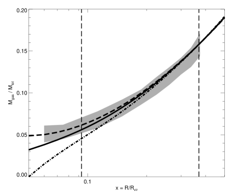
Figure 3: Predicted gas mass fraction profile compared to A496 $90\,\%$ confidence interval (shaded region, see M99). See the text for the meaning of the three curves. The two dashed vertical lines denote the core radius ($R_{c}=0.093\times R_{vir}$) and the radius $R_{1000}$ ($\sim 1\,\rm Mpc$), where the curves are normalised to an observed value of $15.8\,\%$.

2.6 A word on the global and small-scale stability

The question of the stability of the SSCD model against general fluctuations is out of the scope of this paper. I will only briefly comment on this issue. The gas is obviously stable against large-scale convection instability since, as can be seen in a particular case in figure 2, the local polytropic index is, everywhere in cluster, smaller than the adiabatic value of 5/3. This in turn implies that the specific entropy increases monotonically with radius (there is a stratification of the gas in the gravitational potential, according to its specific entropy which ensures the dynamical stability). This is valid for reasonable values of the parameters of the TP and of the surface brightness profile. The figure 4 shows the specific entropy profiles for four different sets of parameters $(\eta,x_{0},x_{c},\beta)$, namely (3,0.05,0.1,2/3) our standard cluster depicted as a solid line (section 2.3), (5,0.01,0.1,2/3) as a dashed line, (3,0.05,0.093,0.7) corresponding to A496, as a dot-dashed line and (5,0.01,0.05,0.636) as a triple-dot-dashed line, corresponding to A2199 (see M99). All the entropy profiles increase with radius, and one can see the effect of the core radius $x_{c}$ and the slope of the surface brightness profile $\beta$ on the profile, notably the models with the larger core radii have a constant entropy core.

Figure 4: Specific entropy profiles for different sets of parameters $(\eta,x_{0},x_{c},\beta)$, where $\eta$ and $x_{0}$ are the parameters of the TP (see section 2) and $x_{c}$ (in units of the virial radius) and $\beta$ are the core radius and the third of the asymptotic slope of the surface brightness profile. The different lines are solid (3,0.05,0.1,2/3), dashed (5,0.01,0.1,2/3), dot-dashed (3,0.05,0.093,0.7), and triple-dot-dashed (5,0.01,0.05,0.636). The last two sets correspond to the surface brightness fits to A496 and A2199 respectively. The profiles are normalized at $x=1$ and the specific entropy scale is relative to an unimportant additive constant.

The question of the stability against small-scale instabilities is a much harder one. However, the gas should be locally stable since, outside the cooling flow, radiation cannot enhance density contrasts and thus begin thermal instability. Moreover,the presence of thermal conduction stabilizes the plasma against small-scale instabilities (Field 1965). This stability is enhanced in the presence of a weak magnetic field (Balbus 1991), and observations (Bagchi et al. 1998) as well as simulations (Rocha-Goncalves & Friaca, 1998) show that weak magnetic fields should exist in the bulk of the ICM.

3 Consequences on the total mass profile in clusters

The total mass and mass density profile of a cluster are of primary importance since, if the mass is dominated by dark matter, they can be directly compared to collisionless numerical simulations. Dubinski & Carlberg (1991) found that the relaxed density profile of their simulated halos were well fitted by a formula derived by Hernquist (1990) from elliptical galaxy dark matter profiles. A systematic study of virialized structures in different cosmological models led Navarro, Frenk & White (1996, 1997, hereafter NFW) to propose an analytic expression for the dark matter density profile, which gives an excellent fit to the spherically-averaged numerical results, not only in all the cosmologies explored, but also in a very large range of mass (from galaxies to rich clusters according to NFW). Further studies (Tormen, Bouchet & White 1996; Huss, Jain & Steinmetz 1999b) extended this result to other cosmologies. Even if no theoretical basis has been yet established for this dark matter profile, it could be the result of the violent relaxation of the dark matter, since collapse with very different initial conditions give rise to the same profile (Huss, Jain & Steinmetz 1999a).

However, NFW’s inner slope has been recently criticized by Moore et al. (1998), who find steeper slopes ($r\propto r^{-1.4}$) in their very high resolution numerical simulations of the formation of clusters, while Kravtsov et al. (1998) find that a profile with a central core (Burkert 1995) fits better observed and simulated dwarf and low-surface brightness early-type galaxies. The reasons for these discrepancies are not yet clear.

Assuming a surface brightness profile of the standard cluster and HSE, the total mass density profile can be computed and the three analytic functions described above fitted to it. Figure 5 plots the mass density profiles obtained and the residuals between the SSCD and analytic profiles.

Although we have made some strong assumptions on deriving the TP, the agreement is within $16\;\%$, and even less than $10\;\%$ in the bulk of the cluster where temperature information is available. This agreement is very good, since the residuals to a NFW fit to CDM simulated cluster halos are on average of $17\;\%$ and $26\;\%$ for a Hernquist profile fit (Tormen et al. 1998).

From figure 5, it appears that the Burkert profile fits better the inner regions, while the NFW profile achieves the best fit in the outer cluster region. However, this can only be stated with real cluster data, and depends on the exact parameter pair ($\eta,x_{0}$) adopted, the overall $15\,\%$ agreement being preserved where temperature data are available. Moreover, to obtain a good fit, the Burkert profile requires a very small core radius of the order of $x_{0}$ ($0.07\times R_{200}$), which is equivalent to no core radius. It is not clear if this effect is due to the core in the analytic X-ray surface brightness profile (since clusters of galaxies can be fit as well by profiles without core like the Sersic profile; Gerbal, private communication) or to the steep inner gradient in the SSCD TP.

Figure 5: Comparison of the total density profile from the SSCD temperature profile and the hydrostatic equilibrium (solid line) with NFW profile (dotted), Hernquist profile (long-dashed) and Burkert profile (dot-dashed). The lower panel shows the percentage difference between these three last models and the SSCD profile. For this particular example, $x_{0}$ was set to $0.05$ and $\eta$ to 3. However, the overall agreement does not depend much on these values, if reasonable.

4 Discussion

The steady-state conduction model described above predicts the relaxed state of a cluster, but tells nothing about an important issue, namely the time taken to reach this steady-state solution. The complete answer to this important question is beyond the scope of this paper, and I will only briefly comment this issue.

Obviously, the time taken to reach the relaxed state will depend on one main factor that governs the inhibition of the heat conduction compared to the classical Spitzer rate: the inhibition factor $f$. Since the model is a steady-state one, note that $f$ disappears naturally from the TP analytic expression when the boundary conditions are introduced into the general solution. The suppression of electronic thermal conduction (hereafter ETC) is a longstanding problem in the theoretical studies of cooling flows (CFs) in clusters of galaxies. The CF interpretation of the central X-ray properties of a great number of clusters (a surface brightness excess compared to a $\beta-$model and a decrease in the central temperature) assumes that gas is removed from the inflow by thermal instabilities and converted into low-mass stars, in view of the lack of obvious repositories for the accreted gas within a Hubble time. This requires a strong suppression of the electronic thermal conduction (ETC), because of its ability to erase thermal instabilities on timescales much shorter than the Hubble time. The suppression must be even higher ($f\leq 10^{-4}$) in weakly magnetized multiphased CF models inferred from observations (Balbus, 1991). There is little doubt that the intracluster magnetic field plays a primordial role in this inhibition. However, the traditional point of view that small-scale tangled magnetic fields could inhibit conduction has been recently severely challenged (Tao 1995, Pistinner & Shaviv 1996; see however Tribble 1989) and seems not to be able to provide enough strong inhibition factors. As already noted by Balbus (1991), collective plasma effects could provide a viable alternative. In particular, Pistinner & Eichler (1998) have recently shown that low-frequency electromagnetic wave instabilities driven by temperature gradients can inhibit sufficiently the ETC in CF to reconcile theory and observations. However, what happens outside the CF is not clear. There, the cooling time is long enough to ensure that thermal instability will have no effect and the temperature gradient is much shallower than in the CF. This last point together with the fact that the magnetic field is expected to decrease with increasing radius suggests that Pistinner & Eichler (1998)’s mechanism is less efficient outside the CF. It is thus worth asking if a conduction-structured temperature profile can accomodate the X-ray data and allow then a simple new analytic model of the ICM TP.

Maybe some answers to the above questions will come from X-ray observations. Chandra recently revealed that in at least two clusters, A2142 (Markevitch et al., 2000) and A3667 (Vikhlinin, Markevitch & Murray, 2000a), dense cool cores are moving with high velocity through the hotter, less dense surrounding gas. A sharp density and temperature discontinuity (called “cold front” by the authors) separates the two phases, while the pressure is continous at the precision level of the satellite. This phenomenon is very interesting, since we seem to observe directly the suppression of transport processes in the ICM. Ettori & Fabian (2000) have argued that the sharp temperature discontinuity requires a suppression of heat conduction relative to the spitzer value by one to three orders of magnitude (depending on the width of the transition region and on the saturation of the conduction). The case is even stronger for A3667, since the width of the density discontinuity is smaller than the inferred Coulomb mean free path, showing directly the suppression of diffusion. In a second paper, Vikhlinin, Markevitch & Murray (2000b) argue that the cold front should be quickly disturbed by Kelvin-Helmholtz instability (while it seems to be stable in the X-ray images over a $\sim 60$ degrees sector), and that the stability is ensured by the surface tension of the magnetic field whose field lines are parallel to the front. In their model, the field lines are initially frozen into the gas and tangled on some scale on each side of the front. The stripping of the cool gas stretches the field lines along the front, which stops the stripping and suppresses transport processes across the front region. They are able to derive a value of the magnetic field strength of $\sim 10\,\rm\mu G$, an order of magnitude higher than other estimates of the ICM field (this can be easily explained by the stretching of the field lines).

This first direct probe of transport processes suppression is very interesting, but it does not mean that the same inhibition is present in all relaxed clusters. In fact, both clusters are in a dynamically perturbed state: A3667 is classified as a spectacular ongoing merger in optical (bimodal galaxies distribution and lensing map), X-rays and radio. A2142 has higly elliptical X-ray isophotes, a centroid shift and an asymmetric temperature map. The great difference in the line-of-sight velocities ($\sim 1840\,\rm km.s^{-1}$) of the two central galaxies argues for a dynamically pertubed system, while the presence of a moderate cooling flow is indicative of the merger being in its late stages. Thus, it is likely that the phenomenon discovered by Chandra is much more indicative of what happens during a merger (high magnetic fields strength, suppression of microscopic transport processes, convection) than when a cluster is in a relaxed state for several Gyrs. As has been said in section 2.3, I do not expect this model to be valid during the violent phases of a merger, but much later, when the cluster had time to relax. Even if a non-negligible percentage of the cluster population is still dynamically active (particularly the more massive), their central parts (say, $R\lesssim R_{vir}/2$) should be described fairly well by the SSCD model. On the other hand, if Chandra and XMM-Newton, with their improved spatial resolution and sensitivity, discover the same phenomenon ongoing in a majority of clusters, even relaxed, the model presented here should not have any physical basis. Numerical simulations at very high simulation without thermal conduction indeed show multiple unerased density and temperature discontinuities for several Gyrs (R. Teyssier, private communication).

5 Acknowledgements

This work constitutes part of the PhD thesis of S.D.S. It is a pleasure to acknowledge useful discussions with Christophe Balland, Stéphane Colombi, Florence Durret, William Forman, Christine Jones, Daniel Gerbal, Mark Henriksen, Barbara Lanzoni, Gastão Lima-neto, Gary Mamon, Maxim Markevitch and Romain Teyssier. I also thank the referee, V. Eke, for pertinent remarks which helped improving the clarity of this paper.

References

- [Arnaud & Evrard(1999)] Arnaud, M., Evrard, A.E., 1999, MNRAS 305, 631
- [Bagchi et al.(1998)Bagchi, Pislar, & Lima Neto] Bagchi, J., Pislar, V., Lima Neto, G.B., 1998, MNRAS 296, L23
- [Balbus(1991)] Balbus, S.A., 1991, ApJ 372, 25
- [Bower et al.(2000)Bower, Benson, Baugh, Cole, Frenk, & Lacey] Bower, R.G., Benson, A.J., Baugh, C.M., Cole, S., Frenk, C.S., Lacey, C.G., 2000, MNRAS submitted, astro-ph/0006109
- [Bryan & Norman(1998)] Bryan, G.L., Norman, M.L., 1998, ApJ 495, 80
- [Burkert(1995)] Burkert, A., 1995, ApJ 447, L25
- [Cavaliere & Fusco-Femiano(1976)] Cavaliere, A., Fusco-Femiano, R., 1976, A&A 49, 137
- [Cavaliere & Fusco-Femiano(1978)] Cavaliere, A., Fusco-Femiano, R., 1978, A&A 70, 677
- [Cavaliere et al.(1997)Cavaliere, Menci, & Tozzi] Cavaliere, A., Menci, N., Tozzi, P., 1997, ApJL 484, L21
- [Cavaliere et al.(1998)Cavaliere, Menci, & Tozzi] Cavaliere, A., Menci, N., Tozzi, P., 1998, ApJ 501, 493
- [Cavaliere et al.(1999)Cavaliere, Menci, & Tozzi] Cavaliere, A., Menci, N., Tozzi, P., 1999, MNRAS 308, 599
- [Chieze et al.(1998)Chieze, Alimi, & Teyssier] Chieze, J.P., Alimi, J.M., Teyssier, R., 1998, ApJ 495, 630
- [Dubinski & Carlberg(1991)] Dubinski, J., Carlberg, R.G., 1991, ApJ 378, 496
- [Ebeling et al.(1997)Ebeling, Edge, Fabian, Allen, Crawford, & Boehringer] Ebeling, H., Edge, A.C., Fabian, A.C., Allen, S.W., Crawford, C.S., Boehringer, H., 1997, ApJ 479, L101
- [Eke et al.(1998)Eke, Navarro, & Frenk] Eke, V.R., Navarro, J.F., Frenk, C.S., 1998, ApJ 503, 569
- [Ettori & Fabian(2000)] Ettori, S., Fabian, A.C., 2000, MNRAS in press, astro-ph/0007397
- [Ettori & Fabian(1999)] Ettori, S., Fabian, A.C., 1999, MNRAS 305, 834
- [Evrard(1990)] Evrard, A.E., 1990, ApJ 363, 349
- [Evrard & Henry(1991)] Evrard, A.E., Henry, J.P., 1991, ApJ 383, 95
- [Evrard et al.(1996)Evrard, Metzler, & Navarro] Evrard, A.E., Metzler, C.A., Navarro, J.F., 1996, ApJ 469, 494
- [Eyles et al.(1991)Eyles, Watt, Bertram, Church, Ponman, Skinner, & Willmore] Eyles, C.J., Watt, M.P., Bertram, D., Church, M.J., Ponman, T.J., Skinner, G.K., Willmore, A.P., 1991, ApJ 376, 23
- [Field(1965)] Field, G.B., 1965, ApJ 142, 531
- [Frenk et al.(1999)Frenk, White, Bode, Bond, Bryan, Cen, Couchman, Evrard, Gnedin, Jenkins, Khokhlov, Klypin, Navarro, Norman, Ostriker, Owen, Pearce, Pen, Steinmetz, Thomas, Villumsen, Wadsley, Warren, Xu, & Yepes] Frenk, C.S., White, S.D.M., Bode, P., Bond, J.R., Bryan, G.L., Cen, R., Couchman, H.M.P., Evrard, A.E., Gnedin, N., Jenkins, A., Khokhlov, A.M., Klypin, A., Navarro, J.F., Norman, M.L., Ostriker, J.P., Owen, J.M., Pearce, F.R., Pen, U.., Steinmetz, M., Thomas, P.A., Villumsen, J.V., Wadsley, J.W., Warren, M.S., Xu, G., Yepes, G., 1999, ApJ 525, 554
- [Gonçalves & Friaça(1998)] Gonçalves, D.R., Friaça, A.C.S., 1998, in: Giuricin, G., Mezzetti, M., Salucci, P. (eds.), Observational Cosmology: the development of galaxy systems, in press, astro-ph/9811264
- [Gull & Northover(1975)] Gull, S.F., Northover, K.J.E., 1975, MNRAS 173, 585
- [Henriksen & White(1996)] Henriksen, M.J., White, R. E., I., 1996, ApJ 465, 515
- [Hernquist(1990)] Hernquist, L., 1990, ApJ 356, 359
- [Hughes et al.(1988a)Hughes, Yamashita, Okumura, Tsunemi, & Matsuoka] Hughes, J.P., Yamashita, K., Okumura, Y., Tsunemi, H., Matsuoka, M., 1988a, ApJ 327, 615
- [Hughes et al.(1988b)Hughes, Gorenstein, & Fabricant] Hughes, J.P., Gorenstein, P., Fabricant, D., 1988b, ApJ 329, 82
- [Huss et al.(1999a)Huss, Jain, & Steinmetz] Huss, A., Jain, B., Steinmetz, M., 1999a, ApJ 517, 64
- [Huss et al.(1999b)Huss, Jain, & Steinmetz] Huss, A., Jain, B., Steinmetz, M., 1999b, MNRAS 308, 1011
- [Irwin et al.(1999)Irwin, Bregman, & Evrard] Irwin, J.A., Bregman, J.N., Evrard, A.E., 1999, ApJ 519, 518
- [Jones & Forman(1984)] Jones, C., Forman, W., 1984, ApJ 276, 38
- [Kaiser(1991)] Kaiser, N., 1991, ApJ 383, 104
- [Kravtsov et al.(1998)Kravtsov, Klypin, Bullock, & Primack] Kravtsov, A.V., Klypin, A.A., Bullock, J.S., Primack, J.R., 1998, ApJ 502, 48
- [Landau & Lifshitz(1959)] Landau, L.D., Lifshitz, E.M., 1959, ”Fluid mechanics”, Course of theoretical physics, Oxford: Pergamon Press, 1959
- [Lea(1975)] Lea, S.M., 1975, Astrophys. Lett. 16, 141
- [Loewenstein(2000)] Loewenstein, M., 2000, ApJ 532, 17
- [Markevitch et al.(1998)Markevitch, Forman, Sarazin, & Vikhlinin] Markevitch, M., Forman, W.R., Sarazin, C.L., Vikhlinin, A., 1998, ApJ 503, 77
- [Markevitch & Vikhlinin(1997)] Markevitch, M., Vikhlinin, A., 1997, ApJ 474, 84
- [Markevitch et al.(1999)Markevitch, Vikhlinin, Forman, & Sarazin] Markevitch, M., Vikhlinin, A., Forman, W.R., Sarazin, C.L., 1999, ApJ 527, 545
- [Metzler & Evrard(1994)] Metzler, C.A., Evrard, A.E., 1994, ApJ 437, 564
- [Mohr et al.(1999)Mohr, Mathiesen, & Evrard] Mohr, J.J., Mathiesen, B., Evrard, A.E., 1999, ApJ 517, 627
- [Moore et al.(1998)Moore, Governato, Quinn, Stadel, & Lake] Moore, B., Governato, F., Quinn, T., Stadel, J., Lake, G., 1998, ApJ 499, L5
- [Navarro et al.(1995)Navarro, Frenk, & White] Navarro, J.F., Frenk, C.S., White, S.D.M., 1995, MNRAS 275, 720
- [Navarro et al.(1996)Navarro, Frenk, & White] Navarro, J.F., Frenk, C.S., White, S.D.M., 1996, ApJ 462, 563
- [Navarro et al.(1997)Navarro, Frenk, & White] Navarro, J.F., Frenk, C.S., White, S.D.M., 1997, ApJ 490, 493
- [Neumann & Arnaud(1999)] Neumann, D.M., Arnaud, M., 1999, A&A 348, 711
- [Pistinner & Shaviv(1996)] Pistinner, S., Shaviv, G., 1996, ApJ 459, 147
- [Pistinner & Eichler(1998)] Pistinner, S.L., Eichler, D., 1998, MNRAS 301, 49
- [Ponman et al.(1999)Ponman, Cannon, & Navarro] Ponman, T.J., Cannon, D.B., Navarro, J.F., 1999, Nature 397, 135
- [Primack et al.(1998)Primack, Bullock, Klypin, & Kravtsov] Primack, J.R., Bullock, J.S., Klypin, A.A., Kravtsov, A.V., 1998, in: Merrit, Valuri, Sellwood (eds.), ASP conference series, Galaxy Dynamics, astro-ph/9812241
- [Rephaeli(1977)] Rephaeli, Y., 1977, ApJ 218, 323
- [Sarazin(1988)] Sarazin, C.L., 1988, “X-ray emission from clusters of galaxies”, Cambridge Astrophysics Series, Cambridge: Cambridge University Press, 1988
- [Schwarzschild(1958)] Schwarzschild, M., 1958, ”Structure and evolution of the stars.”, Princeton, Princeton University Press, 1958.
- [Soker & Sarazin(1990)] Soker, N., Sarazin, C.L., 1990, ApJ 348, 73
- [Spitzer(1965)] Spitzer, L., 1965, “Physics of fully ionized gases”, Interscience Publication, New York
- [Tao(1995)] Tao, L., 1995, MNRAS 275, 965
- [Tormen et al.(1997)Tormen, Bouchet, & White] Tormen, G., Bouchet, F.R., White, S.D.M., 1997, MNRAS 286, 865
- [Tribble(1989)] Tribble, P.C., 1989, MNRAS 238, 1247
- [Valageas & Silk(1999)] Valageas, P., Silk, J., 1999, A&A 350, 725
- [Vikhlinin et al.(1999)Vikhlinin, Forman, & Jones] Vikhlinin, A., Forman, W., Jones, C., 1999, ApJ 525, 47
- [Vikhlinin et al.(2000a)Vikhlinin, Markevitch, & Murray] Vikhlinin, A., Markevitch, M., Murray, S.S., 2000b, ApJ submitted, astro-ph/0008496
- [Vikhlinin et al.(2000b)Vikhlinin, Markevitch, & Murray] Vikhlinin, A., Markevitch, M., Murray, S.S., 2000a, ApJ submitted, astro-ph/0008499 (VMM)
- [Wu et al.(1999)Wu, Fabian, & Nulsen] Wu, K.K.S., Fabian, A.C., Nulsen, P.E.J., 1999, MNRAS in press, astro-ph/9907112
- [Zel’Dovich & Raizer(1967)] Zel’Dovich, Y.B., Raizer, Y.P., 1967, ”Physics of shock waves and high-temperature hydrodynamic phenomena”, New York: Academic Press, 1966/1967, edited by Hayes, W.D.; Probstein, Ronald F.