On the Hardness-Intensity Correlation in Gamma-Ray Burst Pulses

Abstract

We study the hardness-intensity correlation (HIC) in gamma-ray bursts (GRBs). In particular, we analyze the decay phase of pulse structures in their light curves. The study comprises a sample of 82 long pulses selected from 66 long bursts observed by the Burst And Transient Source Experiment (BATSE) on the Compton Gamma-Ray Observatory. We find that at least $57\%$ of these pulses have HICs that can be well described by a power law. A number of the other cases can still be explained with the power law model if various limitations of the observations are taken into account.

The distribution of the power law indices $\gamma$, obtained by modeling the HIC of pulses from different bursts, is broad with a mean of $1.9$ and a standard deviation of $0.7$. We also compare indices among pulses from the same bursts and find that their distribution is significantly narrower. The probability $p$ of a random coincidence is shown to be very small ($<2\times 10^{-5}$). In most cases, the indices are equal to within the uncertainties. These results demand a physical model to be able to reproduce multiple pulses with similar characteristics for an individual burst, but with a large diversity for pulses from an ensemble of bursts. This is particularly relevant when comparing the external versus the internal models.

In our analysis, we also use a new method for studying the hardness-intensity correlation, in which the intensity is represented by the peak value of the $EF_{\rm E}$ spectrum, where $E$ is the energy and $F_{\rm E}$ is the energy flux spectrum. We compare it to the traditional method in which the intensity over a finite energy range is used instead, which may be an incorrect measure of the bolometric intensity. This new method gives stronger correlations and is useful in the study of various aspects of the HIC. In particular, it produces a better agreement between indices of different pulses within the same burst. Also, we find that some pulses exhibit a track jump in their HICs, in which the correlation jumps between two power laws with the same index. We discuss the possibility that the track jump is caused by strongly overlapping pulses. Based on our findings, the constancy of the index is proposed to be used as a tool for pulse identification in overlapping pulses and examples of its application are given.

1. Introduction

The analysis of the spectral and temporal evolution of gamma-ray bursts (GRBs) renders us important clues to the underlying processes giving rise to the phenomenon. The evolution has been studied both over the entire burst, giving the overall behavior, and over individual pulse structures (see, for instance, the review by Ryde 1999a). Pulses are common features in a GRB light curve and appear to be the fundamental constituent of it (see, e.g., Norris et al. 1996, Stern & Svensson 1996). To characterize the spectral evolution, relations between quantities describing different aspects of the evolution have been reported. One important correlation is that between the hardness of the spectrum at a certain time and the integrated flux up to that time, the fluence; the Hardness-Fluence Correlation. In the context of these studies, the hardness is usually given by a ratio of counts in different energy channels or by some characteristic spectral energy, such as the peak energy. Another correlation, which has received attention, is that between the hardness of the spectrum and the instantaneous flux (or intensity); the Hardness-Intensity Correlation (HIC). Most studies concerning these correlations examine them in single pulses and do not compare the behavior of pulses within a burst. However, this has been done for the Hardness-Fluence Correlation by Liang & Kargatis (1996) and by Crider et al. (1999). Corresponding studies of the HIC have been mainly discussed in Kargatis et al. (1995).

The main purpose of these studies is to lead us to an understanding of the emission processes. The mechanisms that generate the bursts are still not known. Many models have been proposed, mostly in the context of two major scenarios involving relativistic shells. In the external model (Mészáros & Rees 1993), a thin shell expands outward after a single release of energy of unknown origin (candidates often considered are cataclysmic stellar collapses or compact stellar mergers). After an initial $\gamma$-ray quiet phase, the shell becomes active, perhaps due to interactions with the external medium. The exact nature of the conversion of the kinetic energy of the bulk motion into $\gamma$-rays is unclear. In the internal shock models, a central engine generates a variable wind and interactions within the wind produce the $\gamma$-ray emission. This is often modeled with a series of relativistic shells that are released, with the fast shells catching up with the slow ones, which leads to the formation of internal shocks.

An approach frequently used in these models is to identify each pulse in the light curve with a single physical event. Depending on the model chosen, this event could be the collision between inhomogeneities in a relativistic wind in the internal models or the “activation” of a region on a single external shell. To validate this reductionistic method, it is essential to find common properties among pulses.

The hardness-fluence correlation was discussed first by Liang & Kargatis (1996) who described it as being an exponential decay of the spectral hardness as a function of the photon fluence. The exponential decay constant appeared to be invariant between pulses in some bursts, which led the authors to suggest that the pulses are created by a regenerative source rather than in a single catastrophic event. However, Crider et al. (1998a) dismissed the apparent invariance as coincidental, and consistent with drawing values out of a narrow statistical distribution, combined with rather large uncertainties in the determination of the exponential decay constant.

The hardness-intensity correlation was discussed first by Golenetskii et al. (1983, hereafter G83). In the present work, we study the HIC for the decay phase of a sample of GRB pulses observed by the Burst and Transient Source Experiment (BATSE) on the Compton Gamma-Ray Observatory (CGRO). We present an extensive comparison of the HIC behavior among pulses from the same burst and between bursts, partly motivated by the behavior of the Hardness-Fluence Correlation. Some of the results have been presented in preliminary form in Borgonovo & Ryde (2000) and Ryde, Borgonovo, & Svensson (2000).

First, in §2 we discuss previous work and results, in which the HIC was often found to be a power law relation. In §3, we present the data we used in the analysis and discuss the observations (§3.1), the sample selection (§3.2), the spectral modeling (§3.3) and the analysis method used (§3.4). In particular, in §3.4.2, we introduce a new method to analyze the HIC. We present our results in §4. The usefullness of our new analysis method is shown in §4.1, and in §4.2 we study individual pulses in GRBs and present the general distribution of their power law indices in §4.2.1. The cases that were not included in the analysis of the distribution, are examined in §4.2.2. In §4.3 we turn to the study of multi-pulse GRBs and investigate cases with several well separated pulses (§4.3.1) and discuss characteristic cases exhibiting track jumps in their HICs. In particular, §4.3.2 presents cases with track jumps occurring in apparently single pulses. In §4.4 we study the power law HICs of pulses within the same burst and compare them to the general distribution from §4.2.1 and find that they are more alike than what is expected from the general distribution. We discuss the final results of our analysis in §5. Our new analysis method is discussed in §5.1 and the track jumps are interpreted as being the result of heavily overlapped pulses in §5.2. Finally, in §6, we discuss how our results impose important constraints on the current physical models and in particular how they will be relevant in comparing external versus internal shock models.

2. The Relation between Hardness and Intensity

The relation between the hardness and the intensity, during the active $\gamma$-ray phase of a GRB, has been well investigated. It has been shown that there is no ubiquitous trend of spectral evolution that can characterize all bursts; several types of behavior exist. Norris et al. (1986) found that the most common trend of spectral evolution is a hard-to-soft behavior over a pulse, with the hardness decreasing monotonically as the flux rises and falls. This conclusion was also arrived at by Kargatis et al. (1994, hereafter K94). A few cases exhibited soft-to-hard and even soft-to-hard-to-soft evolution. Band (1997) studied the data from the four, high time-resolution channels from the Large Area Detectors (LADs) of BATSE. The spectral evolution was analyzed by auto- and cross-correlating light curves from the different energy channels. Most bursts in the sample showed a hard-to-soft behavior.

There are also bursts that do not seem to exhibit any HIC at all, with an apparently chaotic behavior. The main conclusion drawn by Laros et al. (1985) and Jourdain (1990), was that there did not exist a HIC between the spectral evolution and the light curve in their samples (using PVO and APEX data, respectively). Over the whole GRB, there often does not exist any pure correlation, even though the tracks in the hardness-intensity plane are confined to an area from hard and bright to soft and weak, indicating an overall trend of increasing luminosity with hardness (K94). A seemingly chaotic behavior in that plane may be the result of a superposition of several short hard-to-soft pulses that cannot be resolved. Various types of trends have also been seen in a single GRB (e.g., Hurley et al. 1992). The variety of behaviors are also described in Band et al. (1993) and Ford et al. (1995).

Furthermore, there is another behavior in which the intensity and the hardness track each other. This behavior is less common than the hard-to-soft trend and was first noted by G83, who described it quantitatively. They found a power law relation between the instantaneous energy flux, $F$, and the energy parameter $E_{\rm 0}$ derived from modeling the photon spectra using $N_{\rm E}(E)=E^{\alpha}e^{-E/E_{\rm 0}}$, which serves as a measure of the hardness, i.e.,

$$F\propto E_{\rm 0}^{\gamma}.$$ (1)

The power law index $\gamma$ was found to have a typical value of 1.5–1.7. This value is sometimes referred to in the literature as the correlation index.

This analysis was criticized by several workers, including Laros et al. (1985), Norris et al. (1986), and K94. It was speculated that the correlation could possibly be an artifact of the way the hardness was derived from the two-spectral-channel count rates. Furthermore, G83 excluded the hard initial phase of the bursts. Ford et al. (1995) suggested that the low time-resolution may result in the initial, hard behavior being missed. On the other hand, K94 confirmed the description of the HIC made by G83 (eq. [1]), i.e., a power law model of the hardness-intensity correlation (hereafter denoted by PLHIC). They found a power law correlation in approximately half of their cases, but with a substantially wider spread, $\gamma=2.2\pm 1.0$. Furthermore, Strohmayer et al. (1998) investigated the evolution of the peak energy versus the energy flux in the Ginga data and found the PLHIC to be valid here too, with, for instance, $\gamma\sim 3$ for GRB 890929 (in the 2–400 keV energy range).

The present paper concerns mainly the power-law, hardness-intensity correlation during the decay phase of pulses, which is a common behavior. Kargatis et al. (1995) found the PLHIC in 28 pulse decays from 15 bursts, out of a total of 26 GRBs with prominent pulses studied. The distribution of the correlation index peaks at 1.7 and has a substantial spread. A large spread in the PLHIC index was also found by Bhat et al. (1994), who studied 19 time structures with short rise times ($<4$ s) and slow decays, and concluded that most had a good correlation between the hardness and the intensity. The value of $\gamma$ varied from $1.4$ to $3.4$.

Ryde & Svensson (2000a, 2000b) derived the consequences of combining the power law model of the HIC and the exponential model of the Hardness-Fluence Correlation, for the decay phase of GRB pulses. They found a self-consistent, quantitative, and compact description for the temporal evolution of the pulse decay phase. It was shown that, assuming the adopted models are valid, the total photon flux must be $\propto 1/(1+t/\tau)$, where the time $t$ is taken from the start of the decay and $\tau$ is a time constant that can be expressed in terms of the parameters of the two empirical correlations.

3. Data and Methods

3.1. Observations

This work is based on the data taken by BATSE on board the CGRO (Fishman et al. 1989). It consists of eight modules placed on each corner of the satellite, giving full sky coverage. Each module has two types of detectors: the Large Area Detector (LAD) and the Spectroscopy Detector (SD). The former has a larger collecting area and is suited for spectral continuum studies, while the latter was designed for the search of spectral features (lines). For our spectral analysis we used the high energy resolution (HER) background and burst data types from the LADs having 128 energy channels. The burst data have a time-resolution of multiples of 64 ms. The CGRO Science Support Center (GROSSC) at Goddard Space Flight Center (GSFC) provides these data as processed, high-level products in its public archive. The data are available for all the detectors that triggered on the bursts (often 3 or 4 of the detectors closest to the line-of-sight to the burst location). Models of the relevant Detector Response Matrix (DRM) for each observation are also provided (Pendleton et al. 1995). The eight modules of BATSE allow the localization of the GRB, needed for the determination of the DRM, since it is dependent on the source-to-detector axis angle. Finally, we used, for visual inspection of the light curves, the so called concatenated 64-ms burst data, provided by GROSSC, which is a concatenation of the three BATSE data types DISCLA, PREB, and DISCSC.

3.2. Sample Selection

To construct a complete sample of strong bursts, we started by selecting the bursts in the Current BATSE Catalog, up to GRB 990126 (BATSE trigger number 7353), for which it is possible to measure peak fluxes. These are approximately 80% of the totally 2302 observed. Data gaps and/or missing data types are the reason why the peak flux for some bursts are not found. The Current BATSE Catalog is preliminary, but bursts up to GRB 960825 (trigger 5586) are published in the 4th BATSE Catalog (Paciesas et al. 1999). The threshold we chose for accepting a burst was set to a peak flux (50–300 keV in 1.024 s time resolution) of 2 photons s^-1 cm^-2. This selection resulted in a set of 420 bursts.

This set was examined visually, case by case, using the concatenated 64 ms time resolution data. We searched for bursts containing long pulse structures with a general “fast rise-slow decay”, often referred to as “fast rise-exponential decay” (FREDs). No analytical function describing the pulse shape was assumed. The reason for using such a loose definition is to have a sample that is independent of any preconceived idea of the pulse shape. Examples of pulses that are subsequently included in this broad sample are shown in Figure 1.

The identification of the pulse structures may, in some cases, be disputable. A few algorithms for identification have been introduced by, e.g., Li & Fenimore (1996), Pendleton et al. (1997), and Scargle (1998). Norris et al. (1996) developed a method to identify pulses based on assuming stretched exponential pulse shapes. This method was used by, e.g., Crider et al. (1999) to separate pulses, some of which were heavily overlapped. However, all these methods depend on various assumptions. Our sample suffers, on the other hand, from some subjectivity, as we select our pulses visually. However, this should not affect the results, as these are not strongly dependent on the details in this selection process.

For the time-resolved spectroscopy, we will use a high signal-to-noise ratio ($S/N$), which will lead to light curves consisting of only a few broad time bins. We need as many time bins as possible to study the HIC and to arrive at reliable results for the PLHIC index, as we will be determining its distribution (see §4.2 for details). For this purpose we adopt the criterion that the decay phase of the pulses should have at least 5 time bins with $S/N=30$ to be included in the study.

It should be noted that the first and the last time bins could partially cover a time interval that is outside the actual HIC behavior of the decay phase. For the pulse decay, the first time bin studied corresponds to the peak of the pulse, and therefore this time interval might include the transition between the rise and the decay phase. The last time bin might also be a transition interval, i.e., the valley before the rise phase of the next pulse. In the 5-time-bin cases, bearing these qualitative arguments in mind, there are, in the worst case, only 3 central data points that are unaffected and thus are more certain to correctly define the PLHIC index.

The visual inspection resulted in a set of 66 bursts, that is $\approx 3\%$ of the original BATSE catalog. These bursts are presented in Table 1 and they constitute our main sample, which we have striven to make as unbiased and extensive as possible. In the Table, the bursts are denoted by both their BATSE catalog and trigger numbers. The detector from which the data were taken and the number of time bins ($n_{\rm bins}$) selected for fitting are also presented. The pulses studied are identified by the time $t_{\rm max}$ when their count rate is maximal ($t=0$ is the trigger time).

3.3. Spectral Modeling

The central part of the analysis was performed with the WINGSPAN package, version 4.4.1 (Preece et al. 1996a). The spectral fitting was done using the MFIT package, version 4.6, running under WINGSPAN. We always chose the data taken with the detector which was closest to the line-of-sight to the location of the GRB, as it has the strongest signal (see Table 1 for the individual cases). The broadest energy band with useful data was selected, often 25–1900 keV. A background estimate was made using the HER data, which consist of low (16–500 s) time resolution measurements that are stored between triggers. The light curve of the background, during the outburst, was modeled by interpolating these data, roughly 1000 s before and after the trigger, with a second or third order polynomial fit.

To perform detailed time-resolved spectroscopy it has been shown that a $S/N\sim 45$ is needed (Preece et al. 1998). The aim of our spectral analysis, of every time bin, is mainly to determine the peak energy, $E_{\rm pk}$, as a measure of the hardness, and allowing a deconvolution of the count spectrum to find the energy spectrum. Therefore, we accepted a lower $S/N$, sometimes down to 30, but we checked that the results are consistent with higher $S/N$ ratios. This gives us the possibility to study the burst pulses with higher time-resolution, which is of great importance for our study.

The background-subtracted photon spectrum, $N_{\rm E}(E)$, for each time bin, is then determined using a forward-folding technique. An empirical spectral model is folded through the model of the Detector Response Matrix and is then fitted by minimizing the $\chi^{2}$ (using the Levenberg-Marquardt algorithm) between the model count spectrum and the observed count spectrum, giving the best-fit spectral parameters and the normalization. The spectra were modeled with the empirical function (Band et al. 1993):

$$N_{\rm E}(E)=\left\{\begin{array}[]{ll}A\ E^{\alpha}e^{-E/E_{\rm 0}}&\mbox{if $(\alpha-\beta)E_{\rm 0}\geq E$}\\ A^{\prime}E^{\beta}&\mbox{if $(\alpha-\beta)E_{\rm 0}<E$ ,}\end{array}\right.$$ (2)

where $E$ is the energy, $E_{\rm 0}$ is the $e-$folding energy, $\alpha$ and $\beta$ are the asymptotic power law indices, $A$ the amplitude, and $A^{\prime}$ has been chosen to make the photon spectrum $N_{\rm E}(E)$ a continuous and a continuously differentiable function through the condition

$$A^{\prime}=A\left[(\alpha-\beta)E_{\rm 0}\right]^{\alpha-\beta}e^{-(\alpha-\beta)}.$$ (3)

The power law indices were always left free to vary if nothing else is stated. The peak energy, $E_{\rm pk}$, at which the $EF_{\rm E}$-spectrum ($F_{\rm E}=EN_{\rm E}$) is at its maximum, was used as a measure of the spectral hardness instead of $E_{\rm 0}$. They are related by $E_{\rm pk}=(2+\alpha)E_{\rm 0}$ and a peak exists only when $\beta<-2<\alpha$. The fitting procedure has then 4 free parameters: $A$, $\alpha$ and $\beta$, and $E_{\rm pk}$. The photon spectrum arrived at is model-dependent. However, as equation (2) often gives a good model of the spectra, the photon spectrum found by deconvolving the count spectrum should correspond well with the true photon spectrum. For every time bin, the instantaneous integrated energy flux $F$ was found by integrating the modeled energy spectrum over the available energy band of the detector.

These procedures have now given us, beside the spectral parameters, a data set of peak energies and energy flux values for every time bin of the pulse decays. Note, however, that due to the low energy cut-off of the detector, in practice only $E_{\rm pk}$ values $\gtrsim 40$ keV can be reliably determined. For this reason, it is often the case that a few time bins, at the end of the pulse decays, are not used in our studies of the hardness-intensity temporal evolution.

3.4. HIC Analysis Method

3.4.1 Statistical Analysis

Different statistical approaches can be used to test whether a power law model is adequate to describe the hardness-intensity data, and to determine its best-fit parameters and their likely uncertainties. Here, we once again used the minimization of the merit function $\chi^{2}$. If the uncertainties of the measurements are known, a model-independent determination of the goodness-of-fit can be obtained. This is done typically by calculating the probability $Q$ of exceeding by chance the $\chi^{2}$ minimum obtained (see, e.g., Press et al., 1992). Data points were weighted using the uncertainties in the $E_{\rm pk}(t)$ estimation, which are usually much larger than the intensity uncertainties. We found in too many cases unrealistic values of $Q\approx 1$. The most likely explanation is that the uncertainties derived from the spectral fitting are overestimated. Their usefulness is therefore doubtful. One possible cause of this could be the strong correlation observed between some of the Band et al. function parameters, particularly between $\alpha$ and $A$ (see, e.g., Lloyd & Petrosian 2000). Such a correlation could partly be due to an artifact of the fitting. However, to distinguish this from a physical relation between the parameters, a more detailed study has to be undertaken.

The power law model can be linearized by taking the logarithms of the intensity and the hardness measure. The power law index then becomes the slope of the linear relation, and ordinary linear regression can be used to fit the data. After this transformation, in most cases, the $E_{\rm pk}$-measurement uncertainties are approximately equal and, since the detector energy channels are approximately equally spaced on a logarithmic scale, more symmetric error bars are expected. In addition, the HIC data points are more evenly distributed. Thus, assuming that the uncertainties are exactly equal, i.e., using the unweighted method, we can obtain the coefficient of determination, $R^{2}$, i.e., the square of the linear correlation coefficient. For any given $R^{2}$, $P_{N}(R^{2})$ is the probability that $N$ measurements of two uncorrelated variables would give a coefficient larger than $R^{2}$. This probability is a measure of how significant the linear correlation is.

The tests $R^{2}$, $\chi^{2}$, and the like, do not have information about the temporal order of the data points, so obviously one should not infer anything about the temporal evolution of the HIC from these statistics. However, most pulse decays in our sample that have a very good PLHIC also show a good tracking behavior, i.e., the temporal evolution in the hardness-intensity plane is monotonic, aside from random fluctuations that can be attributed to the measurement uncertainties. Nevertheless, this generalization must be taken with caution in cases with low correlation coefficients. Another important aspect not measured by these tests is whether the residuals show any particular trend or feature. In this respect, we analyzed in detail the cases with many time bins and concluded that the data are consistent with the power law model.

To fit the data directly one can employ a non-linear regression numerical algorithm (with the Levenberg-Marquardt method). The outcome is essentially the same as in the linear regression and will not be presented here.

In conclusion, the difference between the indices obtained using weighted and non-weighted fittings was, in most cases, within the estimated uncertainties. No significant difference was obtained either from our various statistical analyses of the two data sets. We will show the results derived from the non-weighted, linear fittings, but we checked that our conclusions are independent of this choice.

3.4.2 The $\varphi$-method for studying the HIC

The limited spectral coverage of the detector used might affect the assigned measure of the bolometric flux, i.e., the energy-integrated flux, as a substantial fraction of the flux could be lost, especially when the spectrum has a broad shape or peaks close to the boundaries of the detector. A second problem, when one aims at studying the correlation within single pulses in the light curve, arises from the fact that the observed spectra may contain contributions from other pulses, for instance, previous pulses which still contribute with soft photons, and unresolved, overlapping pulses. Furthermore, additional, separate soft components (Preece et al. 1996b) could also alter the measured flux value and thus weaken the correlations. All this can affect the analysis by changing the shape of the spectrum.

This motivated us to introduce a new representation of the HIC, which might resolve some of these complications (see also Ryde et al. 2000). The value of $EF_{\rm E}$ at $E_{\rm pk}$ can be used as a representation of the energy-integrated flux as it, under some circumstances, is proportional to the total flux. This quantity will be denoted by $\varphi$ (see Fig. 9a) and the PLHIC can be studied as

$${\varphi}\propto E_{\rm pk}^{\eta},$$ (4)

where $\eta$ is the new PLHIC index. This discussion is limited to the cases where the $EF_{\rm E}$ peak actually exists within the detector band $[E_{\rm min},E_{\rm max}]$, which most often is the case (Band et al. 1993). In the most common case, where $E_{\rm max}>(\alpha-\beta)E_{\rm pk}/(\alpha+2)$, the proportionality between ${\varphi}$ and $F=\int F_{\rm E}dE$ becomes

$$\frac{F}{\varphi} \equiv k(\alpha,\beta,y_{\rm min},y_{\rm max})=\frac{e^{(\alpha+2)}}{(\alpha+2)^{\alpha+2}}\times$$

$$[\Gamma(\alpha+2)\{P(\alpha+2,\alpha-\beta)-P(\alpha+2,y_{\rm min})\}+$$

$$\frac{(\alpha-\beta)^{\alpha-\beta}y_{\rm max}^{\beta+2}-(\alpha-\beta)^{\alpha+2}}{(\beta+2)e^{\alpha-\beta}}],$$

where $y_{\rm min}=(\alpha+2)E_{\rm min}/E_{\rm pk}$, and $y_{\rm max}=(\alpha+2)E_{\rm max}/E_{\rm pk}$. $\Gamma(\alpha)$ and $P(\alpha,y)$ are the gamma function and the incomplete gamma function, respectively (see, e.g., Press et al. 1992). In the case that $\alpha$ and $\beta$ depend weakly on $E_{\rm pk}$, the only $E_{\rm pk}$ dependence in $k(\alpha,\beta,y_{\rm min},y_{\rm max})$ is in $y_{\rm min}$ and $y_{\rm max}$. In particular, when the flux integration is chosen to be over the whole energy range from $0$ to $\infty$, there will be no dependence at all. Therefore, $\varphi$ should be a better representation of the bolometric flux for the study of the HIC.

4. Results of the Analysis

4.1. Correspondence between the $F$ and $\varphi$

Before discussing the results of the HIC analysis, we will compare the HIC relation as given by equation (1), but using the parameter $E_{\rm pk}$ as a measure of the hardness (§ 3.3)

$$F\propto E_{\rm pk}^{\gamma},$$ (6)

and the new representation given by equation (4). For this comparison, we use a subset of 47 pulse decays (in 39 bursts) from the sample, which have been selected as having good PLHICs, i.e., the cases having a relative uncertainty $\Delta\eta/\eta\leq 0.15$ and marked with an $A$ in Table 2 (see § 4.2 for a discussion of this choice). For each pulse decay we analyzed the spectral evolution and determined both the $\gamma$ and the $\eta$ values. When comparing the coefficients of determination given by the two methods we found that in $83\%$ of the cases $R^{2}_{\eta}$ is greater than $R^{2}_{\gamma}$. To find whether the observed difference is significant, we made use of Fisher’s $z$-transformation

$$z=\frac{1}{2}\ln\left(\frac{1+R}{1-R}\right),$$ (7)

where each $z$ is approximately normally distributed, with a standard deviation $\sigma(z)\approx 1/\sqrt{N-3}$, and $N$ being the number of data points (see, e.g., Press et al. (1992)). Individual differences are not significant, but the difference between the respective mean values, $\bar{z}_{\eta}-\bar{z}_{\gamma}$, was found to be positive at a significance level of $P$-value $=0.015$ (the $P$-value is the probability that the value of the test statistic is as extreme as it is, with the null hypothesis being true). This implies that the new $\varphi$-method does give better correlations.

The relation between the two PLHIC indices $\gamma$ and $\eta$ for all pulse decays in the subset $A$ is shown in Figure 2. A linear fit to these data gives $\gamma=(0.96\pm 0.09)\eta+(0.08\pm 0.16)$. This shows that there is a good average correspondence between the two methods. All these results convinced us to use the $\varphi$-method in the subsequent studies.

4.2. The PLHIC index of Single Pulses

The results of the fitting of the bursts in our main sample are presented in Table 2. Apart from the power law indices $\eta$ and $\gamma$ obtained, it shows $R_{\eta}^{2}$ and its associated probability $P_{N}(R^{2}_{\eta})$, $R_{\gamma}^{2}$, and the relative uncertainty $\Delta\eta/\eta$.

From these bursts we select and study the subset $A$ for which the hardness-intensity relation is well fitted by a power law model. This decision is not trivial and the concern was to set a reliable rejection level to select those cases that are consistent with the model. The probability $P_{N}(R^{2})$ could be used for this purpose (see §3.4.1). In practice, the relative uncertainty of the slope in the linear regression, either $\Delta\eta/\eta$ or $\Delta\gamma/\gamma$, gives a more convenient measure (at least when the range of slope values is not close to zero). We found empirically that, for our set, a rejection level of $P_{N}(R^{2}_{\eta})<0.001$ (usually considered as highly significant) is approximately equivalent to selecting cases with $\Delta\eta/\eta\leq 0.15$. This level was chosen to define the subset $A$ in Table 2. We used the $\eta$ indices in our selection because the $\varphi$-method gives better correlations (see §4.1), but almost the same subset would be reached using $\Delta\gamma/\gamma\leq 0.2$. The selection of the rejection level was a trade-off between choosing a high level and reducing significantly the sample size, or a low one that would increase the statistics but may allow cases that are likely also to have large systematic errors.

4.2.1 The Distribution of PLHIC Indices among Bursts

To study the distribution of some parameter associated with GRB pulses, one should consider that pulses within the same burst may not be independent. Furthermore, they may have a different distribution of the parameter values considered as compared to their distribution for pulses over the full burst sample, i.e. the general distribution. We will show below that at least the latter is true for the $\gamma$ and $\eta$ indices. In that case, a small sample can be easily biased by taking many values from a multi-pulse burst. Therefore, to estimate the general distribution of the PLHIC indices when two or more pulses were measured in the same burst, only one was taken. To select it, we chose the one that shows the best correlation in terms of the probability $P_{N}(R^{2}_{\eta})$. This method is consistent with the fact that very often only one pulse, among many in the burst, is found suitable for this analysis, i.e., we are already disregarding noisy and therefore poorly correlated cases. On the other hand, since indices are very similar within bursts, as will be found below, other criteria, such as a random selection, produced no significant differences.

We studied how the resulting distributions depend on the chosen rejection level $\Delta\eta/\eta$. When trying to estimate the underlying probability distribution of any sample, care must be taken that the measurement uncertainties do not contribute significantly. Allowing cases with larger relative uncertainties, i.e., worse PLHIC cases, results in almost identical mean values but larger standard deviations. This is to be expected, since the data have now a larger intrinsic dispersion that is added to (convolved with) the real distribution. For later use in our studies, it is important to set a fairly high rejection level, in order to have a good estimate of the real dispersion.

Thus, taking from the main sample one pulse per burst and only the cases with $\Delta\eta/\eta\leq 0.15$, defines the subset of 39 pulses marked with $B$ in Table 2, for which we will study the general distribution of the indices (note that $B\subset A$). Using the $F$-method, the mean value of the PLHIC index is $\bar{\gamma}=1.9\pm 0.1$ with a standard deviation of the sample $\sigma_{\gamma}=0.72\pm 0.08$. We also provide the expected deviations of these estimators to facilitate the comparisons. Using the $\varphi$-method the mean value and dispersion for the PLHIC indices are $\bar{\eta}=2.0\pm 0.1$ and $\sigma_{\eta}=0.68\pm 0.08$. The weighted fittings mentioned in (§ 3.4.1) produce very similar results. For example, the values obtained with that method are $\bar{\eta}_{\rm w}=2.15\pm 0.10$ and $\sigma_{\eta_{\rm w}}=0.80\pm 0.09$. The differences are of the same order as the estimated uncertainties.

These results should only be compared with the ones obtained in studies of the decay part of pulses. As mentioned above, Kargatis et al. (1995) found a central value of $\bar{\gamma}\sim 1.7$, which is somewhat lower than ours. However, their sample of 28 pulses was taken from 15 multi-pulse GRBs. This might produce a slower convergence to the real mean value. In fact, if we allow more than one pulse per burst in our statistics, we get a $\bar{\gamma}=1.8\pm 0.1$ for 47 pulses from 39 bursts (subset $A$ in Table 2). Note that although in many bursts only one pulse was found suitable for our studies, it does not mean that there were no other pulses present. A real distinction between single and multi-pulse bursts would be difficcult to achieve, especially as we do not know what a single pulse really looks like.

In Figure 3, histograms of the subset $B$ of measured PLHIC indices, $\gamma$ and $\eta$, are displayed. The sample is too small for a detailed study of the underlying distributions. However, for later use in this work (§ 4.4), we test the assumption of a normal distribution for both indices. We use the Geary test of normality (see, for instance, Devore 1982), a simpler but more powerful test procedure than the $\chi^{2}$ test, that is specific for this purpose. It is based on the ratio of the average absolute deviation to the square root of the average square deviation, given by

$$U=\frac{\sqrt{\pi/2}\sum_{i}|X_{i}-\bar{X}|/n}{\sqrt{\sum_{i}(X_{i}-\bar{X})^{2}/n}}.$$ (8)

For samples larger than 20 the Geary test can be approximated by a two-tailed $Z$-test, where the null hypothesis is that the underlying distribution is normal and the standardized $U$ is

$$Z=\frac{U-1}{0.2661/\sqrt{n}}.$$ (9)

For the $\eta$ and $\gamma$ samples, high $P$-values are found, 0.73 and 0.34 respectively, implying that the approximation of a normal distribution can be reliably used.

4.2.2 The Excluded Cases

We found, using the $R^{2}$ statistics, that $57\%$ of the main sample of pulse decays (subset $A$) could be described by a power law at a highly significant confidence level. At the level of significance of only $P_{N}(R^{2}_{\eta})\leq 0.01$ (approximately equivalent results would be obtained using $\Delta\eta/\eta<0.2$) the number increases to about $75\%$. Since the $R^{2}$ coefficient is not a very sensitive test, these percentages should be taken as approximative.

There are several possible causes for some of the cases showing poor power law correlations. We could often recognize problems that were affecting our analysis of the HIC in a systematic way, making uncertain any conclusion about the applicability of the power law, or any other model for that matter. In some cases, for instance, the $EF_{E}$-spectrum peaks at higher energies than the observed band. However, the numerical algorithm finds an $E_{\rm pk}$ value within the energy window using $\beta>-2$. As the whole spectrum evolves towards lower energies, at some point the absolute maximum enters the observation window but the overall evolution of the HIC is poorly fitted by a power law.

Although the Band et al. function proved to be a very flexible model to describe most GRB spectra, it presents difficulties when trying to fit some particularly broad shaped cases (see, e.g., Ryde 1999b). In a graphical $EF_{E}$ vs. $E$ representation, a typical zig-zag evolution is obtained, accompanied by opposite changes in $\alpha$ and $\beta$. A similar effect occurs when either of the latter two parameters is loosely constrained by the data. Although in these cases an overall track behavior is apparent, PLHIC fits result in poor $R^{2}$ coefficients, and residuals show an uneven dispersion.

Furthermore, the selected pulse decay could also turn out not to be a single pulse decay after all, even if it appears to be. Overlapping, “hidden” secondary pulses in the light curve produce a characteristic effect in the HIC evolution that, under some circumstances, can be recognized and used as a pulse identification aid. This will be discussed in detail in § 4.3.1. Finally, some cases could actually have another HIC behavior. An investigation of alternative models will be presented elsewhere (Ryde & Svensson 2000c, in preparation).

4.3. The PLHIC Index of Multi-pulse Bursts

We will now study the distribution of the PLHIC indices within a single burst. In order to increase the sample, we look for additional pulses, with 4 time bins, in the GRBs listed in Table 1. The expanded sample of multi-pulse bursts includes 4 of these shorter pulses, but in each case there is a longer pulse to compare with. The pulses from GRB 950104 (trigger 3345) are also included, based on the discussion in § 4.3.1. In this way, we increase the number of multi-pulse cases from 11 to 15 GRBs. They all show at least moderately good correlations.

Apart from these cases, a set of pulses, apparently single, but having a track jump in the HIC will be studied in detail. They are noted with TJ in Table 1 and can be interpreted as consisting of several pulses (see also Borgonovo & Ryde 2000).

4.3.1 Bursts with Several Well-separated Pulses

The sample of GRBs which have two or more well-separated pulses is shown in Table 3. As an example, we present the case of GRB 921207 (trigger 2083) in Figure 4. This burst has been examined by many workers (e.g., Ford et al. (1995), Crider et al. 1998a , cr99 (1999), and Ryde & Svensson 1999a ) and is one of the best BATSE cases available for this type of study, with two bright and long pulses. In Figures 4$c$ and $d$, the hardness-intensity evolution is shown. The decay phases of both pulses show very good correlations and the power law indices are equal to within the estimated uncertainties. ¿From the point of view of the PLHIC, the first pulse structure is consistent with being a single pulse. This is also the conclusion of Ryde & Svensson (1999) who studied various aspects of the spectral/temporal evolution of GRB pulses. However, with the pulse identification method proposed by Norris et al. (1996) this pulse structure can be modeled as a superposition of two individual, overlapping, stretched exponential pulses (see Crider et al.  1999). In the present spectral analysis there is no indication of this, although one cannot rule it out.

As another example, the overall evolution of GRB 970420 (trigger 6198) is shown in Figure 5. While the spectral evolution during the rise phases does not seem to follow any clear trend, again in this case we observe a good PLHIC during the decay phases. The slopes are equal to within the estimated uncertainties (see Table 2).

In Figure 6 the light curve of GRB 950104 (trigger 3345) is shown. The section after the peak at $t\simeq 6$ s can be interpreted as having two pulses which overlap closely. An indication of the existence of a secondary pulse can be found as follows. The assumption has to be made that the rise and decay phases of individual pulses are strictly monotonic and then we calculate whether the deviation can be attributed to the Poisson noise in the signal. For that purpose, a simple test would be to find the significance of the count difference between the suspected peak and the nearby valleys (see Li & Fenimore 1996):

$$C_{\rm peak}-C_{\rm valley}\geq N_{\sigma}\sqrt{C_{\rm peak}},$$ (10)

where $N_{\sigma}$ is the number of $\sigma$ standard deviations. In the case of GRB 950104, we found a significance $N_{\sigma}=3.2$, within the interval $3\leq N_{\sigma}\leq 5$ recommended for the test, i.e., marginally significant. Figures 6 $a$ and $b$ show two count time history plots of this burst; one with a time binning with $S/N=40$ and the other with the 64-ms time resolution of the concatenated data. The spectral evolution of the peak energy corresponding to the time binning in panel ($a$) is also shown in panel ($c$). Initially, the second decay has approximately the same PLHIC index as the first one. It then makes a change into a parallel track. Checking the 64 ms count rate time history, one can see that this track jump coincides with the presence of the small secondary peak (marked with an arrow) which is hidden in the low time resolution binning. Even though the significance of the peak is somewhat marginal, the agreement with the slope of the first pulse track makes the case more compelling for the presence of overlapping pulses. The power law indices obtained for the tracks are $\eta_{1}=0.77\pm 0.05$, $\eta_{2}=0.79\pm 0.03$, and $\eta_{3}=0.76\pm 0.05$, equal to within the estimated uncertainties.

Note that the $E_{\rm pk}$ uncertainties derived from the spectral fittings (Fig. 6c) are heavily overestimated. This is a common characteristic of the track jump cases, and it will be discussed in §5.1.

4.3.2 Apparently Single Pulses

The three cases presented here seem to be single pulses as seen from the 64 ms light curves. These pulses are taken from GRB 910927 (trigger 829), GRB 960912 (trigger 5601), and GRB 970925 (trigger 6397), respectively and they are shown in Figures 6 and 7. All three behave similarly to the case GRB 950104 discussed above. We have modeled their decay evolution with two power laws and a track jump. The result of the fittings are shown in Table 4.

Although there is no clear indication of secondary peaks, in the case of GRB 970925, a small “bump” in the light curve (more easily noticed in a log-linear graph) coincides with the track jump. The measured indices, $\eta_{1}=0.77\pm 0.15$ and $\eta_{2}=0.86\pm 0.05$, are again equal to within the uncertainties, as in the other two cases.

In the case of the pulse decay in GRB 910927, and only in this case, the fitted results are obtained with the parameter $\beta$ frozen for all points. Although the qualitative behavior is the same, it produces a sharper transition between the tracks. Note that the spectral evolution (Fig. 7c) during the decay of the first pulse, given by the bins 2–4, seems to follow the same track as do the points numbered 14–16. It could therefore be that the last points, in fact, belong to the decay of the first pulse and that the pulse peaking at bin 9 has a fast decline and is superimposed in the middle of the dominating, long first pulse.

4.4. The Distribution of the PLHIC Index within GRBs

An interesting question is how the distribution of the HIC index within a burst compares to the general distribution as presented in §4.2. Our set of multi-pulse bursts was introduced in §4.3 and listed in Table 3. It consists of 35 pulses taken from 15 GRBs. We can see, from Tables 2 and 3, that the PLHIC indices are, in most cases, very similar. To estimate the probability of having similar indices within bursts purely by chance, it will be assumed first that the set of random variables $X_{i}\in\{\eta\}$ (or $\{\gamma\}$) have approximately a normal distribution $X_{i}\sim N(\bar{\eta},\sigma_{\eta})$, as has been justified in section §4.2.1. Let $Y\equiv X_{i}-X_{j}$ be the difference between two indices from the same burst. If they are independent, then $Y\sim N(0,\sqrt{2}\sigma_{\eta})$. A hypothesis test can be performed to see whether $\sigma^{2}_{0}\equiv 2\sigma^{2}_{\eta}$ is the true variance. Thus, choosing the null hypothesis $H_{\rm 0}\!:\sigma^{2}=\sigma^{2}_{0}$, we will use first the test statistic

$$\chi^{2}_{a}=\frac{(n-1)s^{2}}{\sigma^{2}_{0}},$$ (11)

where $s$ is the standard deviation and $n-1$ is the number of degrees of freedom.

This test has the advantage of using a standard probability distribution function, but special care must be taken when considering the cases where 3 (or more) pulses have been measured within a burst, let us say A, B, and C. We can form three differences, but obviously one of them will not be independent of the others. An approximation could be done adjusting the number of degrees of freedom, but then equation (11) will not be strictly valid. Numerical simulations convinced us that, at least in this case, this is not a good approximation. The results shown in Table 5 from the $\chi^{2}_{a}$ test were obtained selecting pairs (A, B) and (B, C). We verified that our conclusions are not affected by this choice. The dispersions expected assuming independency are $\sqrt{2}\sigma_{\gamma}=1.02$ and $\sqrt{2}\sigma_{\eta}=0.96$, and the standard deviations obtained are $s_{\gamma}=0.39$ and $s_{\eta}=0.30$, respectively. In all cases, the $P$-values are very small for both indices $\gamma$ and $\eta$. Therefore we can confidently reject $H_{\rm 0}$ in favor of the alternative hypothesis, i.e., the distribution of PLHIC indices over a single burst is narrower than the one observed over the whole sample of GRBs.

In Figures 8$a$ and $b$ we illustrate how all possible index differences, taking pulses in temporal order, compare with the normal distribution assumed in $H_{\rm 0}$. We had to run a numerical simulation to find the non-standard probability distribution for the variance of all index differences. We define the test statistic

$$T_{a}\equiv\sum_{i=1}^{N}\;\;\sum_{j=1}^{M_{i}-1}\sum_{k=j+1}^{M_{i}}(X_{ij}-X_{ik})^{2},$$ (12)

where $N$ is the number of bursts in the sample and $M_{i}$ is the number of measured pulses within burst $i$. This test is obviously independent of the order in which the differences are taken. Using a Monte Carlo method, we found the probability density function of $T_{a}$ assuming, as before, that each index $X_{ij}$ follows the general distributions found in § 4.2.1, and using the normal approximation. The results of this second test are presented in Table 5. Again, $P$-values are very small for both indices, confirming the conclusions of the previous test. The purpose of using first the $\chi_{a}^{2}$ test as an approximation is that, having a known analytical solution, it can estimate very low probabilities without being limited by computational time.

We have now established that the distribution of indices among pulses within a burst is narrower than the one between pulses of different bursts. Figures 8$a$ and $b$ show that most uncertainties in our sample are much smaller than the dispersion of the general distribution. Note also that most error bars cover the origin, suggesting that individual index differences are not significant. We will now consider whether the index dispersion within a burst could be attributed almost entirely to the stochastic uncertainties. Figure 8$c$ and $d$ show the standardized residuals of all possible differences $Y_{i}$ between pulses of the same burst in our sample. The proportion of data points within integer multiples of $\sigma$ is consistent with a Gaussian distribution, except for an “outlier” in the $\eta$ set, at number 14. This point and point number 12 are both differences taken against the second pulse of GRB 950624 (pulse 3648b; see Table 2) which is a fairly weak but long pulse. It precedes and slightly overlaps a strong pulse (3648c), which could produce a systematic error in our measurements. Note also, however, in Table 2 that comparing the estimated index uncertainties almost always $2\gtrsim\Delta\gamma/\Delta\eta\gtrsim 1$. One exception is this case where $\Delta\gamma/\Delta\eta\approx 8$. This is why for the $\gamma$ differences (Fig. 8c) the corresponding point is within $\pm 1\sigma$. The cause of the large deviation is most likely due to a casual alignment of data points that resulted in an underestimation of the $\Delta\eta$ uncertainty. This fact stresses the importance of having high selection requirements. If we had tried to expand our sample to include even weaker or shorter pulses, with fewer time-bins, it would have been at the cost of increasing the risk of systematic errors. Since these are difficult to identify and quantify, they can easily distort the statistics.

Assuming that the indices are constant within a burst, we will estimate the probability to exceed the observed dispersion. The uncertainties will be assumed to be drawn from a normal distribution. Therefore the index differences $Y\in\{X_{ij}-X_{ik}\}$ should follow $Y_{i}\sim N(0,\sigma_{i})$, where each $\sigma_{i}^{2}$ is found by adding the corresponding $X_{i}$ variances. We define, in a similar way as before, a test statistic

$$T_{b}\equiv\sum_{i=1}^{N}\;\;\sum_{j=1}^{M_{i}-1}\sum_{k=j+1}^{M_{i}}\frac{(X_{ij}-X_{ik})^{2}}{\sigma^{2}_{ij}+\sigma^{2}_{ik}},$$ (13)

where the summation considers all possible differences. Since not all differences are independent, we have to solve it numerically. On the other hand, if we restrict the sum to independent terms

$$\chi^{2}_{b}\equiv\sum_{i=1}^{N}\;\;\sum_{j=1}^{M_{i}-1}\frac{(X_{ij}-X_{ij+1})^{2}}{\sigma^{2}_{ij}+\sigma^{2}_{ij+1}},$$ (14)

the test becomes a standard $\chi^{2}$ statistic.

The results of these last two tests are summarized in the second part of Table 5. For the $\gamma$ indices we found relatively low $P$-values for both tests, but we consider that, at the 0.07 probability given by the more precise test ($T_{b}$), the hypothesis of invariance of the $\gamma$ index is marginally acceptable. The results concerning the $\eta$ indices depend on the inclusion or rejection of pulse number 3648b mentioned above. The outlier term completely dominates the sums in equations (14) and (13). Its inclusion gives $P$-values $\ll 10^{-5}$ for both tests. Obviously, a $9\sigma$ difference can not be explained in terms of Gaussian uncertainties. On the other hand, rejecting this data point, we obtained high $P$-values, implying that the observed differences between $\eta$ indices are most likely due to the measurement uncertainties.

Finally, considering again Figure 8, it is apparent that while the $\eta$ differences have approximately a zero mean, the $\gamma$ differences tend to be negative, i.e., later pulses have generally larger indices. Taking the averages of the standardized residuals, the means are $-0.037$ and $-0.49$ for the $\eta$ and $\gamma$ differences, respectively. We calculated, in the $\gamma$ case, whether the non-zero mean deviation is significant. For that purpose a similar statistic to equation (13) was used, but without squaring the terms. We found a 0.03 probability (two-sided level) to exceed the observed value assuming a zero mean, indicating a significant deviation.

5. Discussion

5.1. Comparison between the $F$ and $\varphi$ methods

The introduction of the $\varphi$-method for HIC studies was motivated in § 3.4.2. It was shown (Fig. 2) that there is a good average correspondence between the indices $\gamma$ and $\eta$. The scatter around an exact correspondence was to be expected. As mentioned above, additional flux components can be contributing to the estimated flux affecting the resulting PLHIC index. The $\varphi$-method is less dependent on this. Furthermore, the exact equivalence between the power law indices is valid only in the case that $\alpha$ and $\beta$ do not vary with $E_{\rm pk}$, which they do in many bursts. Furthermore, the flux $F$ is found by integrating the deconvolved spectrum and the deconvolution is model-dependent. This could introduce additional scatter into the PLHIC relation.

We have used both $F$ and $\varphi$ in our studies and the results lead basically to the same general conclusions, albeit some important differences should be noted. In our analysis of the index distribution within a single burst (Fig. 8), the $\eta_{i}-\eta_{j}$ differences show a narrower distribution than the corresponding $\gamma_{i}-\gamma_{j}$. In § 4.1 we concluded that the new approach gives better correlations. This implies that, in general, the estimated uncertainties of $\eta$ are smaller. Even so, when testing the null hypothesis of index invariance using equation (13), $H_{0}$ is marginally accepted in the $\gamma$ case (probability $p=7\%$) , while it is fully consistent for $\eta$ ($p=64\%$). We have also shown that the general distributions of $\eta$ and $\gamma$ (Fig. 3) are very similar. Their means and dispersions are equal to within the uncertainties, thus covering about the same range of values. All these facts strongly suggest that the underlying distribution within a single burst is indeed very narrow, that the observed larger spread can be attributed to the uncertainties of the measurements, and that a better estimator of the HIC will consequently reduce this spread. Obviously, this is also valid for the determination of the general distribution, but in this case the observed reduction is comparable to the standard deviation uncertainties.

We also discussed in § 4.4 that within a burst, later pulses seem to have larger $\gamma$ indices, although the difference is not highly significant. This trend is not observed in the $\eta$ values. This might be a systematic error overcome by the $\varphi$-method. Later pulses are usually softer, and therefore closer to the lower energy limit of observation. See, for example, the burst trigger 2083 in Figure 4. The greater slope of the second pulse PLHIC, quantified in panel ($c$), is of the same order as the one obtained in comparative simulations of the methods, assuming a constant spectral shape (i.e., $\alpha$ and $\beta$ fixed in eq. [2]). A larger sample is needed to verify the trend, but this suggests that indeed the new method is less affected by the detector energy window.

The $\varphi$-method thus provides a better way of studying detailed features in the observed HICs. Finally, the better invariance within a burst shown by the $\eta$ indices may allow us to recognize hidden pulses in the light curve of the burst, as will be discussed next.

5.2. Track Jumps and Overlapping Pulses

Figure 9$a$ illustrates the observed evolution of $\varphi(E_{\rm pk})$ along a track during the decay phase of a single pulse. When many pulses are present in the light curve of a burst, and even though there is no apparent general trend during the rise phases, we have found that they follow almost parallel tracks during the decay phases. To observe this behavior clearly, it is necessary that the pulses do not overlap significantly. Also, they must be bright and long enough to establish the direction of the track, see section 3.2.

In section 4.3.1, we presented the case GRB 950104 (trigger 3345) with marginally separated pulses, which exhibits a track jump in its HIC. We consider this as a limiting case, where it can still be claimed, from the analysis of the time history alone, that a secondary pulse is present (see Fig. 6a). This fact, together with the slope agreement, within the uncertainties, between the first pulse track and the tracks in the second pulse, makes it an interesting example among the track jump cases.

Analogous HIC behaviors were found in a further three cases, shown in section 4.3.2, but there no visible secondary pulse was seen. For instance, GRB 970925 (trigger 6397; see Fig. 6$b$) shows an apparent change in the overall decay, which could be due to a hidden pulse. However, there is an implicit assumption of the pulse shape being an exponential. Nevertheless, in the present study we do not want to make such assumptions concerning the shape of the pulses.

A simple interpretation of the track jump is to assume that it is produced by an overlapping secondary pulse. From this point of view, this feature is present also in cases like GRB 970420 (trigger 6198) shown in Figure 5. The only difference is that there we can resolve the individual pulses in the light curve. Due to the strong temporal evolution of $E_{\rm pk}$ observed in all presumed single pulses, two overlapping pulses will show, if all pulses within a burst have similar spectral shapes and behaviors, a continuous change in the way the individual spectral shapes overlap each other. These fundamental shapes may be fairly constant, but the combined evolution in the $EF_{\rm E}$–$E$ plane will give the impression of an overall change. In Figure 9$b$, we illustrate such a model of two spectral components. The components follow identical tracks during their decay phases. As the peak energy of the main pulse declines, a harder component appears at the rise phase of the secondary pulse. At some point this component starts to dominate the total spectrum and the fitting routine finds a better $\chi^{2}$ value, shifting the Band et al. function parameters to peak at a higher $E_{\rm pk}$, and the jump occurs. Note that due to the broad shape of the spectrum, the changes in the values of the asymptotic slopes of the Band et al. function are an artifact of the fitting.

The uncertainties of the parameter $E_{\rm pk}$ are estimated by evaluating the confidence region around the $\chi^{2}$ minima of the fits. When the spectral shape has a local maximum close to the absolute maximum, an overestimation of the $E_{\rm pk}$ uncertainties occurs. These uncertainties are of the same order as the energy interval that separates the tracks. But the very good alignment of the data points along the tracks indicates that the shape features are real and not a random occurrence.

In studies of the spectral/temporal evolution, other workers (e.g., Kargatis et al. (1995); Liang & Kargatis (1996)) have fixed the parameters $\alpha$ and $\beta$ to reduce the estimated uncertainties of $E_{\rm pk}$. For instance, the parameter values of the time-integrated spectrum can be used. Such a solution provides more “stable” $E_{\rm pk}$ values, but a case like GRB 950104 (trigger 3345) would be missed. It smoothes out the track jump in such a way that a single, steeper track is obtained for the whole decay. Also a coarser time binning (see Ryde & Svensson 2000c) makes the jump “invisible”.

Based on this discussion we propose a pulse identification method for cases of extensive overlap, under the following assumptions. First, the GRB pulses are assumed to actually follow a PLHIC during their decays. We may not observe this because the pulse is too weak or short, because the observation energy window is inadequate, or because there are unresolved secondary pulses present. Second, we have to assume that the correlation index is approximately constant within a burst. We have shown four cases where the pulse separation is evident in the hardness-intensity plane but not as clearly in the light curve. This pulse separation is not so easily accomplished by traditional methods (see §3.2), but can be used as an auxiliary tool. However, to identify track jumps with some confidence, the distance between tracks should be larger than the observed dispersion along individual tracks. Also a minimum number of points on each track is needed to produce a reasonable fit.

We found few cases in our BATSE sample that meet these requirements. However, future instrumentation will allow higher time-spectral resolution and these criteria may then have a wider application.

6. Constraints on GRB Models

The conditions that determine a particular PLHIC index may depend, in principle, on many physical factors of the emitting system, e.g., the density, composition, radiation processes, geometry, etc. This fact is reflected by the broad distribution of the indices $\eta$ and $\gamma$ that we found when studying pulses from different bursts (see Fig. 3). The internal models (see, e.g., Kobayashi et al. (1997), Daigne & Mochkovitch (1998)) rely on the assumption of a random distribution of some shell parameters, such as the density, the kinetic energy or the momentum, to explain the chaotic time histories observed but also to obtain high efficiencies. The sequence of collisions and merging between different shells follows a stochastic process that will hardly consistently reproduce identical physical conditions in each emitting shock front. On the contrary, most probably it will statistically reflect almost the same diversity of conditions found when we observe many bursts. Based on these models, one would expect a similar parameter dispersion when pulses are taken from the same or different bursts. On the other hand, it is conceivable that in the case bursts were very anisotropic, differences due to the viewing angle would be enhanced by the relativistic beaming and this could become a dominating factor. In spite of that, the internal models will still need to produce a narrow PLHIC index dispersion within a burst. The approximate constancy of the PLHIC index is more easily explained in terms of a single system where an active region is regenerated or different parts become active at different times, as it is assumed in many variations of the external shock scenario (see, e.g., Fenimore et al. (1999)).

7. Conclusions

We have introduced a new method to study the hardness-intensity correlation in GRBs. Instead of measuring the energy flux, we use the value of $\varphi=EF_{\rm E}$ at $E=E_{\rm pk}$, which differs by an approximately constant factor. This method has many advantages. First of all, the correlations become stronger. Second, the $\varphi$-method is less dependent on the spectral window of the observations. Third, it disregards the effects of soft components and additional weak pulses with spectra which overlap the one being studied. In cases where the spectrum consists of two approximately equally strong components (from different pulses) the $\varphi$-method captures the evolution of one of the components and disregards the second. These cases produce broad spectra which are not very well modeled by the Band et al. function. Fourth, the resulting flux measure, $\varphi$, is less sensitive to the details of the deconvolution, e.g., the uncertainties in the spectral shape.

We constructed a sample of prominent GRB pulses consisting of 82 cases. Of these, we found that at least $75\%$ exhibited moderately good (or better) PLHICs. Among the poorly correlated cases, we could recognize some technical problems that were affecting our analysis. Thus, the applicability of the PLHIC model may be even larger.

A specific feature was found in the hardness-intensity evolution of some seemingly single pulses. In the HIC diagram of these cases, there is a sharp transition from one power law track to a second, both with the same PLHIC index. This feature is denoted as a track jump and in half of the cases, it coincides with a weak feature in the light curve. This could be explained as being produced by overlapping pulses. The track jumps in the HIC diagram reveal the transition to a new pulse and it can be used as an aid for pulse identification.

We established that the distribution of the PLHIC index is narrower for pulses within a burst than the distribution for pulses from different bursts. The latter can be approximated by a normal distribution. The dispersion within a burst could be entirely attributed to the stochastic uncertainties and the index is thus practically invariant.

These results demand a physical model to be able to reproduce multiple pulses from an individual burst with similar characteristics. At the same time, however, pulses from an ensemble of different bursts should exhibit a diversity that is larger. This is particularly relevant when comparing the external versus the internal models. The latter models require a large diversity of properties of the colliding shells giving rise to the pulses, both within a burst and among bursts.

Changes in the observational conditions among different bursts, such as viewing angle, could possibly account for the disparity between the index distributions. These matters will be considered in future research.

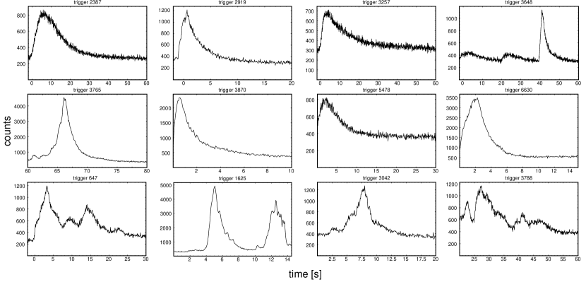
Figure 1.— Examples of pulses from our sample. The upper two rows show fairly smooth, typical pulses selected. However, we also include some cases that show some apparent sub-structure, as the ones in the bottom row. See Table 1 for further information.

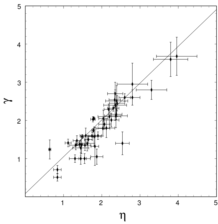
Figure 2.— Relation between the correlation indices $\gamma$ and $\eta$ for 47 pulses with a good PLHIC, i.e., $\Delta\eta/\eta\leq 0.15$ (marked as subset $A$ in Table 2). The straight line shows a weighted linear fit $\gamma=(0.96\pm 0.09)\eta+(0.08\pm 0.16)$ to the data. This shows that there is a good correspondence between the two methods, i.e., using the intensity measures $F$ and $\varphi$, respectively.

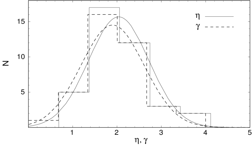
Figure 3.— Distributions of the hardness-intensity correlation indices, $\gamma$ and $\eta$, for a set of 39 pulses (marked in Table 2 as subset $B$). This set is defined by all the sample cases with $\Delta\eta/\eta\leq 0.15$, but restricted to only one pulse per burst (see text for more details). Both index distributions can be approximated by normal distributions with $\bar{\gamma}=1.9\pm 0.1$ and $\sigma_{\gamma}=0.72\pm 0.08$, and $\bar{\eta}=2.0\pm 0.1$ and $\sigma_{\eta}=0.68\pm 0.08$ respectively.

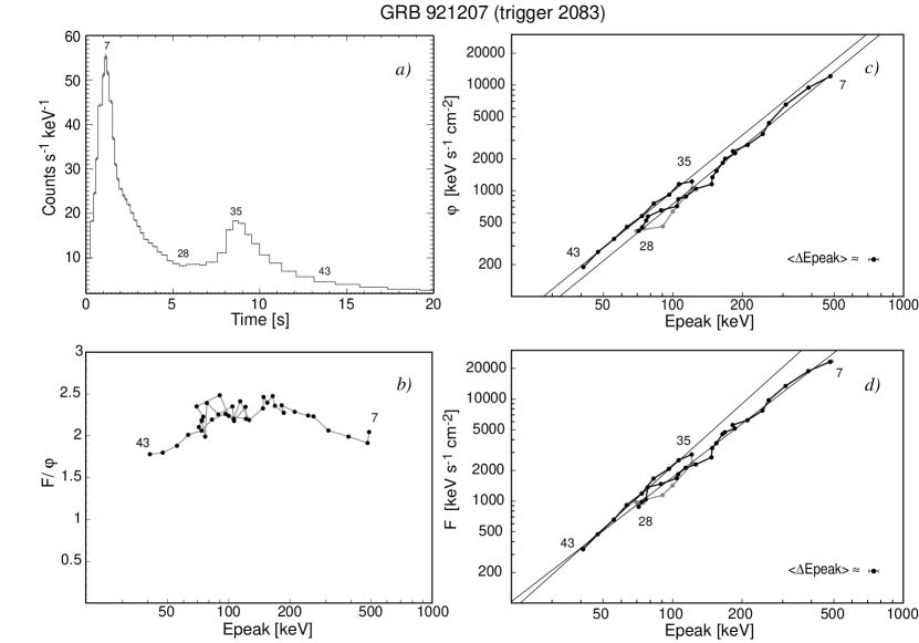
Figure 4.— $a$) Count rate time history showing the time binning used to study the spectral evolution of GRB 921207 (trigger 2083). A few bin numbers are shown. The last few bins are not included in this study because the $E_{\rm pk}$ estimation is very uncertain as the peak of the spectrum approaches the low energy limit of the detector. This is often seen when $E_{\rm pk}\lesssim 40$ keV. $b$) Time evolution of the ratio $F/\varphi$. The integration of the flux was made over the energy range 24–2000 keV. The $F$-measure will suffer from window problems at high and low energies. $c$) The PLHIC measured with the $\varphi$-method. The evolution during the decay phases is shown with dark dots. Error bars are excluded for clarity, and only a typical average value is shown separately. The numbers refer to the time-bins in panel ($a$). We find, for each pulse decay, the power law indices $\eta_{1}=1.78\pm 0.04$ and $\eta_{2}=1.77\pm 0.06$. $d$) Same as ($c$), now using the $F$-method. The corresponding indices are $\gamma_{1}=1.74\pm 0.04$ and $\gamma_{2}=2.03\pm 0.07$. Note that, as in general, the similarity between the PLHIC indices of pulses within a burst is more evident using the $\varphi$-method.

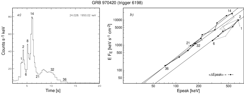
Figure 5.— $a$) Count time history of GRB 970420 (trigger 6198) showing the binning used to study the spectral evolution. The second pulse (at bin number 8) actually consists of two close-lying pulses, which are seen in the 64-ms data. $b$) The peaks of the instantaneous spectra at successive times are represented by dots. Error bars are excluded for better visibility, and only a typical average value is shown separately. The numbers refer to the time-bins in panel ($a$). During the decay phases (dark dots), the HIC follows very good power laws with indices $\eta_{1}=2.25\pm 0.20$, $\eta_{2}=2.40\pm 0.15$, and $\eta_{3}=2.20\pm 0.15$, equal to within the estimated uncertainties.

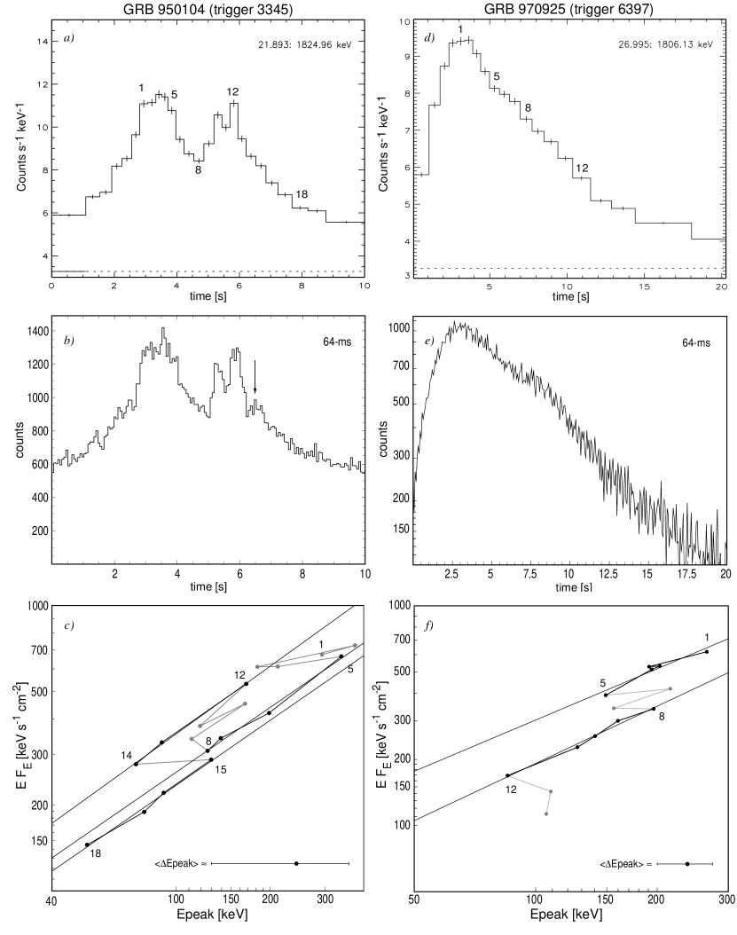
Figure 6.— Spectral evolution of GRB 950104 (trigger 3345) and GRB 970925 (trigger 6397). $a$), $d$) Photon time history showing the binning used to study the spectral evolution ($S/N=40$). The dashed line indicates the background level. $b$) The same time interval using 64-ms time resolution data. A secondary peak is present at $t\simeq 6.5$s. See the text for details. $c$) The peaks of the instantaneous spectra at successive times are represented by dots. The numbers refer to the time-bins. The first pulse decay follows a power law with index $\eta_{1}=0.77\pm 0.06$. The second pulse decay initially follows the same law, within the measurement uncertainties, with $\eta_{2}=0.78\pm 0.025$. A track jump occurs at the time of the rise of the secondary peak in the light curve and then the spectral peak evolution continues on a parallel track $\eta_{3}=0.81\pm 0.05$ while the light curve decays again. Error bars are excluded for better visibility, and only a typical average value is shown separately. The fitting procedure largely overestimates the uncertainties in these cases. $e$) The burst trigger 6397 at 64-ms time resolution. $f$) Evolution of the peak energy during the pulse decay phase. As in the previous case ($c$), the whole decay presents a poor hardness-intensity correlation, but it can be divided into parallel tracks with very good HICs and equal indices to within the uncertainties ($\eta_{1}=0.80\pm 0.15$ and $\eta_{2}=0.90\pm 0.07$). Note the presence of a small “bump” at $t\simeq 7.5$ s, i.e., at bins number 6 and 7.

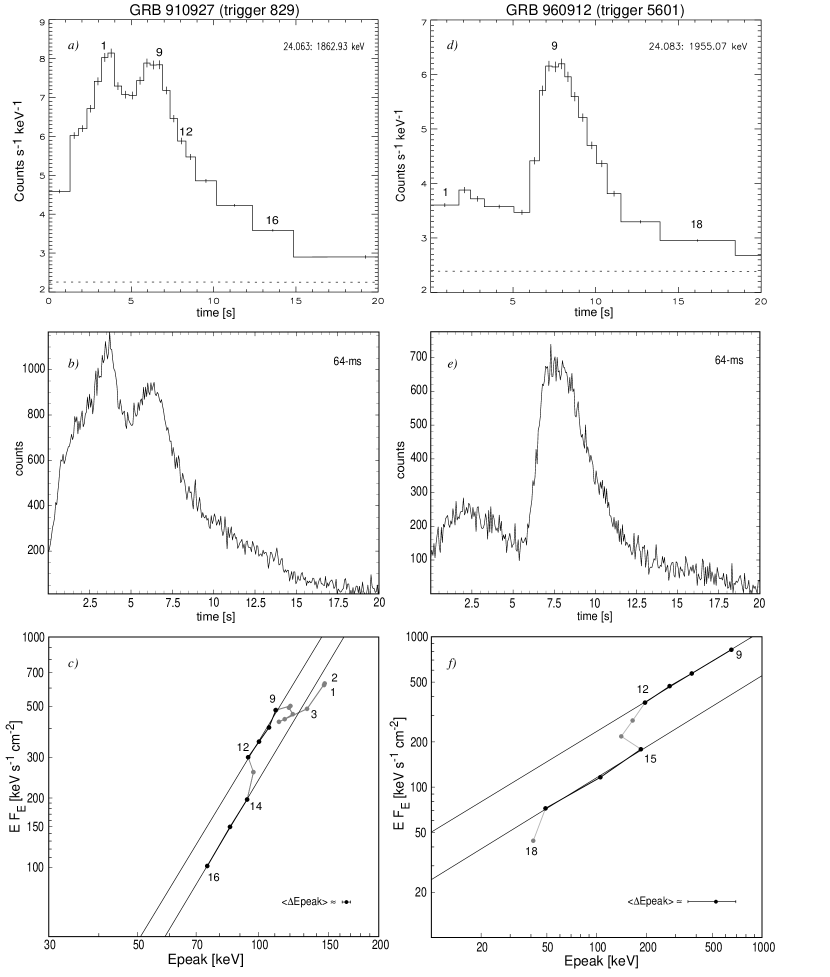
Figure 7.— Spectral evolution of GRB 910927 (trigger 829) and GRB 960912 (trigger 5601). $a$), $d$) Photon time history showing the binning used to study the spectral evolution with signal-to-noise levels of 40 and 30, respectively. The dashed line indicates the background level. $b$), $e$) Time history at 64-ms time resolution. $c$) Evolution of the peak energy during the pulse decay phase. As in the previous examples, it can be divided into two parallel tracks with indices $\eta_{1}=2.95\pm 0.3$ and $\eta_{2}=2.91\pm 0.07$. Note that the first pulse, that has its peak at bin 2, seems to follow the track defined by the last three data points numbered 14–16. It could therefore be that the pulse peaking at bin 9 has a fast decline and is amid the decay of a dominating, long pulse. $f$) The same for burst trigger 5601, with indices $\eta_{1}=0.675\pm 0.01$ and $\eta_{2}=0.675\pm 0.04$, equal to within the uncertainties. In both cases the high-resolution light curve shows no clear sign of a “hidden” pulse.

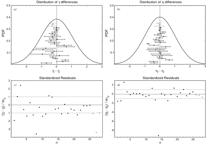
Figure 8.— $a$), $b$) Probability density function (PDF) of the differences, formed between the PLHIC indices $\gamma$ and $\eta$, from pulses of different bursts (which are obviously independent) follows approximately the normal distributions shown by the solid curves. Their dispersion are $\sqrt{2}\sigma_{\gamma}=1.02$ and $\sqrt{2}\sigma_{\eta}=0.96$, respectively. Differences between indices within a single burst, e.g., $\eta_{i}-\eta_{j}$, should follow the same distribution if they were independent too. The graph shows instead that the 25 differences, taken from 35 pulses studied, have a smaller dispersion (all differences are done in temporal order). The standard deviations calculated are $s_{\gamma}=0.39$ and $s_{\eta}=0.30$. Note that the dispersion and the error bars of the $\eta$ differences are slightly smaller than those of $\gamma$. Furthermore, most error bars cover the origin, implying equal values to within the uncertainties. The ordinate position of the points is arbitrary, but the order of the studied bursts is temporal (see Table 3). The extra points in grey represent cases belonging to the track jump sample (Table 4). $c$), $d$) Standardized residuals are shown. Assuming that the indices are constant within each burst, the observed spread should be entirely due to the measurement uncertainties, presumably normally distributed. Dashed lines indicate the $\pm 1\sigma$ region. Note the “outlier” at number 14, related to the second pulse of GRB 950624 (labeled 3648b in Table 2). Note also that $\gamma$ differences tend to be negative, i.e., later pulses tend to have higher indices. This is likely to be an effect of the limited energy window. See the text for discussion.

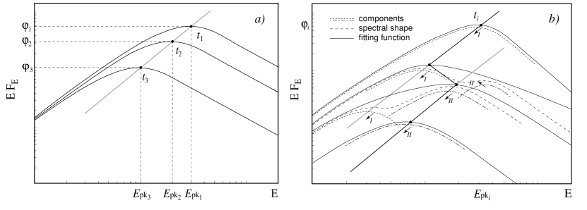
Figure 9.— $a$) Schematic spectral evolution in the $EF_{\rm E}$ representation. During pulse decays, the spectral peaks evolve in time following a power law. $b$) Schematic two-component model explaining track jumps. Each component evolves in a similar way, following approximately parallel tracks when decaying. However, the second is delayed in time and the “jump” occurs when it overcomes the first component. See the text for further details.

Table 1Sample of 82 pulses in 66 GRBs

Burst	trigger	LAD	$t_{\rm max}[s]$	$n_{\rm bins}$
GRB910627	451	4	5.6	5
GRB910897	647	0	3.2/14.0	8/8
GRB910814	676	2	51.5	5
GRB910927	829	4	6.3	8
GRB911016	907	1	1.4	14
GRB911031	973	3	2.7/24.2	19/12
GRB911104	999	2	4.0	5
GRB911118	1085	4	8.7	14
GRB911126	1121	4	21.9/24.7	8/6
GRB911202	1141	7	4.0/9.7	8/8
GRB920221	1425	7	5.9	5
GRB920502	1578	5	8.0	9
GRB920525	1625	4	5.0/12.6	12/5
GRB920623	1663	4	17.1	10
GRB920718	1709	7	2.1	6
GRB920830	1883	0	0.8	7
GRB920902	1886	5	8.3	10
GRB921003	1974	2	1.3	5
GRB921123	2067	1	21.2	8
GRB921207	2083	0	1.1/8.6	22/9
GRB930201	2156	1	14.9	12
GRB930425	2316	1	14.4	12
GRB930612	2387	6	5.9	19
GRB931221	2700	3	53.4	8
GRB940329	2897	4	8.2/24.0	5/5
GRB940410	2919	6	0.5	13
GRB940429	2953	3	5.7/13.0	9/7
GRB940623	3042	1	7.8	14
GRB940708	3067	6	2.4	19
GRB941026	3257	0	4.5	13
GRB941121	3290	0	39.7	10
GRB950104	3345	1	5.8	7
GRB950325	3480	3	0.2	10
GRB950403	3491	3	7.7	16
GRB950403	3492	5	5.3	15
GRB950624	3648	3	2.7/22.7/40.9	6/5/10
GRB950818	3765	1	66.1	12
GRB950909	3788	3	27.2	14
GRB951016	3870	5	0.5	8
GRB951102	3891	2	33.3	7
GRB951213	3954	2	0.8	16
GRB960113	4350	1	13.8	6
GRB960124	4556	5	1.8/3.6	6/5
GRB960530	5478	2	1.9	7
GRB960531	5479	0	52.5	5
GRB960708	5534	5	1.7	5
GRB960804	5563	4	1.4	6
GRB960807	5567	0	11.8	10
GRB960912	5601	0	1.9	10
GRB961001	5621	2	3.9/7.2	6/5
GRB961009	5628	1	10.2	5
GRB961102	5654	5	19.0	14
GRB961126	5697	6	0.6	6
GRB970111	5773	0	8.1/17.3/19.4	8/5/6
GRB970223	6100	6	8.2	16
GRB970420	6198	4	4.2/6.1/9.9	5/8/5
GRB970815	6335	7	0.8	7
GRB970925	6397	7	2.8	12
GRB971127	6504	2	3.2	5
GRB980125	6581	0	47.6	7
GRB980301	6621	1	32.7	6
GRB980306	6629	1	215	6
GRB980306	6630	3	2.1	9
GRB980821	7012	0	2.9	6
GRB990102	7293	6	3.3	10
GRB990123	7343	0	37.7	8

Table 2The HIC power law indices for 78 pulses in 62 GRBs

Pulse	$\eta$	$\gamma$	$R^{2}_{\eta}$	$R^{2}_{\gamma}$	$P_{N}(R^{2}_{\eta})$	$\Delta\eta/\eta$	Comments
451b	$1.36\pm 0.24$	$1.38\pm 0.33$	0.9166	0.8509	$1.0\,\times{{10}^{-2}}$	0.18
647a	$2.12\pm 0.22$	$1.80\pm 0.25$	0.9382	0.8868	$7.6\,\times{{10}^{-5}}$	0.10	$A$
647b	$2.54\pm 0.18$	$1.40\pm 0.30$	0.9692	0.7888	$9.2\,\times{{10}^{-6}}$	0.071	$A,B$
676	$3.30\pm 0.40$	$2.80\pm 0.25$	0.9561	0.9788	$4.0\,\times{{10}^{-3}}$	0.12	$A,B$
907	$2.34\pm 0.15$	$2.54\pm 0.20$	0.9512	0.9422	$3.1\,\times{{10}^{-9}}$	0.064	$A,B$
973a	$1.45\pm 0.21$	$1.28\pm 0.21$	0.7371	0.6821	$2.6\,\times{{10}^{-6}}$	0.14	$A,B$
973b	$0.84\pm 0.10$	$0.71\pm 0.11$	0.8590	0.8041	$1.5\,\times{{10}^{-5}}$	0.12	$A$
999	$1.90\pm 0.10$	$1.60\pm 0.10$	0.9905	0.9825	$3.9\,\times{{10}^{-4}}$	0.053	$A,B$
1085	$1.79\pm 0.025$	$2.05\pm 0.04$	0.9978	0.9954	$<10^{-10}$	0.014	$A,B$
1121a	$1.30\pm 0.15$	$1.00\pm 0.10$	0.9318	0.9172	$1.0\,\times{{10}^{-4}}$	0.12	$A,B$
1121b	$1.17\pm 0.20$	$1.10\pm 0.14$	0.9150	0.9385	$2.8\,\times{{10}^{-3}}$	0.17
1141a	$0.84\pm 0.10$	$0.51\pm 0.10$	0.9198	0.8117	$1.7\,\times{{10}^{-4}}$	0.12	$A,B$
1141b	$0.86\pm 0.15$	$0.76\pm 0.15$	0.8781	0.8400	$5.9\,\times{{10}^{-4}}$	0.17
1425	$2.70\pm 0.50$	$2.55\pm 0.50$	0.8922	0.9060	$1.6\,\times{{10}^{-2}}$	0.19
1578	$2.80\pm 0.40$	$2.95\pm 0.55$	0.8696	0.8038	$2.5\,\times{{10}^{-4}}$	0.14	$A,B$
1625a	$2.37\pm 0.30$	$2.12\pm 0.31$	0.8584	0.8188	$1.5\,\times{{10}^{-5}}$	0.13	$A,B$
1625b	$2.23\pm 0.58$	$1.95\pm 0.55$	0.8315	0.8057	$3.1\,\times{{10}^{-2}}$	0.26
1663	$1.45\pm 0.15$	$1.00\pm 0.15$	0.9139	0.8342	$1.6\,\times{{10}^{-5}}$	0.10	$A,B$
1709	$2.30\pm 0.15$	$2.32\pm 0.08$	0.9865	0.9946	$6.9\,\times{{10}^{-5}}$	0.065	$A,B$
1883	$2.39\pm 0.29$	$2.51\pm 0.40$	0.9303	0.8783	$4.5\,\times{{10}^{-4}}$	0.12	$A,B$
1886	$3.80\pm 0.45$	$3.60\pm 0.45$	0.8965	0.8786	$3.3\,\times{{10}^{-5}}$	0.12	$A,B$
1974a	$2.20\pm 0.30$	$2.10\pm 0.30$	0.9537	0.9495	$4.3\,\times{{10}^{-3}}$	0.14	$A,B$
2067	$2.60\pm 0.15$	$2.60\pm 0.10$	0.9852	0.9902	$1.0\,\times{{10}^{-6}}$	0.058	$A,B$
2083a	$1.78\pm 0.04$	$1.74\pm 0.04$	0.9889	0.9890	$<10^{-10}$	0.022	$A,B$
2083b	$1.77\pm 0.06$	$2.03\pm 0.07$	0.9915	0.9926	$1.7\,\times{{10}^{-8}}$	0.034	$A$
2156	$1.55\pm 0.15$	$1.00\pm 0.13$	0.9117	0.8460	$1.4\,\times{{10}^{-6}}$	0.097	$A,B$
2316	$0.64\pm 0.23$	$0.60\pm 0.30$	0.4395	0.2870	$1.8\,\times{{10}^{-2}}$	0.35
2387	$1.09\pm 0.17$	$0.83\pm 0.33$	0.7035	0.2695	$7.2\,\times 10^{-6}$	0.16
2700	$1.70\pm 0.45$	$1.70\pm 0.45$	0.7067	0.6867	$8.9\,\times{{10}^{-3}}$	0.26
2897b	$1.24\pm 0.45$	$1.47\pm 0.40$	0.7344	0.7886	$6.4\,\times{{10}^{-2}}$	0.36
2897c	$1.42\pm 0.40$	$2.20\pm 0.50$	0.8177	0.8179	$3.5\,\times{{10}^{-2}}$	0.28
2919	$1.39\pm 0.38$	$2.20\pm 0.50$	0.5478	0.3954	$3.8\,\times{{10}^{-3}}$	0.27
2953a	$1.61\pm 0.30$	$1.28\pm 0.27$	0.8094	0.7577	$9.5\,\times{{10}^{-4}}$	0.19
2953b	$1.46\pm 0.45$	$1.24\pm 0.41$	0.6785	0.5777	$2.3\,\times{{10}^{-2}}$	0.31
3042	$1.38\pm 0.88$	$1.07\pm 0.90$	0.3809	0.7875	$1.9\,\times{{10}^{-1}}$	0.64
3067	$1.35\pm 0.10$	$1.47\pm 0.13$	0.8963	0.8820	$8.6\,\times{{10}^{-10}}$	0.074	$A,B$
3257	$2.80\pm 0.20$	$2.60\pm 0.20$	0.9573	0.9268	$7.0\,\times{{10}^{-9}}$	0.071	$A,B$
3290	$1.12\pm 0.08$	$1.41\pm 0.10$	0.9625	0.9560	$5.5\,\times{{10}^{-7}}$	0.071	$A,B$
3480	$2.07\pm 0.15$	$1.90\pm 0.13$	0.9686	0.9653	$2.7\,\times{{10}^{-7}}$	0.072	$A,B$
3491	$1.75\pm 0.09$	$1.59\pm 0.10$	0.9600	0.9477	$<10^{-10}$	0.051	$A,B$
3492	$1.65\pm 0.10$	$1.50\pm 0.10$	0.9378	0.9272	$3.2\,\times{{10}^{-9}}$	0.061	$A,B$
3648a	$1.03\pm 0.30$	$1.87\pm 0.50$	0.7705	0.7647	$2.1\,\times{{10}^{-2}}$	0.29
3648b	$0.64\pm 0.03$	$1.24\pm 0.25$	0.9930	0.9027	$2.5\,\times{{10}^{-4}}$	0.047	$A$
3648c	$1.42\pm 0.08$	$1.38\pm 0.08$	0.9743	0.9749	$1.2\,\times{{10}^{-7}}$	0.056	$A,B$
3765	$2.40\pm 0.20$	$2.45\pm 0.20$	0.9438	0.9217	$1.4\,\times{{10}^{-7}}$	0.083	$A,B$
3788	$1.67\pm 0.26$	$1.35\pm 0.35$	0.7691	0.5571	$3.8\,\times 10^{-5}$	0.16
3870	$0.78\pm 0.15$	$0.76\pm 0.20$	0.7927	0.7147	$3.0\,\times{{10}^{-3}}$	0.19
3891	$1.80\pm 0.18$	$1.58\pm 0.25$	0.9498	0.8922	$2.0\,\times{{10}^{-4}}$	0.10	$A,B$
3954	$1.25\pm 0.20$	$0.97\pm 0.21$	0.7759	0.5907	$6.6\,\times 10^{-6}$	0.16	(1)
4350	$0.82\pm 2.8$	$1.0\pm 4.3$	0.0207	0.0137	$7.9\,\times{{10}^{-1}}$	3.4
4556a	$1.50\pm 0.30$	$1.20\pm 0.30$	0.8756	0.7937	$6.1\,\times{{10}^{-3}}$	0.20
4556b	$1.47\pm 0.17$	$1.36\pm 0.23$	0.9621	0.9180	$3.2\,\times{{10}^{-3}}$	0.12	$A,B$
5478	$1.87\pm 0.16$	$1.05\pm 0.20$	0.9664	0.8835	$7.1\,\times{{10}^{-5}}$	0.086	$A,B$
5479	$1.06\pm 0.26$	$1.03\pm 0.30$	0.8423	0.7785	$2.8\,\times{{10}^{-2}}$	0.25
5534	$0.55\pm 0.14$	$0.96\pm 0.17$	0.8415	0.9138	$2.8\,\times{{10}^{-2}}$	0.25
5563	$2.35\pm 0.30$	$2.40\pm 0.40$	0.9226	0.9042	$2.3\,\times{{10}^{-3}}$	0.13	$A,B$
5567	$3.96\pm 0.53$	$3.68\pm 0.50$	0.8750	0.8761	$7.0\,\times{{10}^{-5}}$	0.13	$A,B$
5621a	$1.26\pm 0.26$	$0.97\pm 0.32$	0.8521	0.6893	$8.6\,\times{{10}^{-3}}$	0.21
5621b	$1.32\pm 0.16$	$1.35\pm 0.12$	0.9570	0.9773	$3.8\,\times{{10}^{-3}}$	0.12	$A,B$
5628	$1.05\pm 0.25$	$0.75\pm 0.20$	0.8503	0.7850	$2.6\,\times{{10}^{-2}}$	0.24
5654	$2.00\pm 0.50$	$2.00\pm 0.50$	0.5549	0.5728	$2.2\,\times{{10}^{-3}}$	0.25
5697	$3.75\pm 0.70$	$4.50\pm 0.70$	0.8804	0.9057	$5.6\,\times{{10}^{-3}}$	0.19
5773a	$1.56\pm 0.15$	$1.35\pm 0.14$	0.9573	0.9397	$2.5\,\times{{10}^{-5}}$	0.096	$A,B$
5773b	$1.82\pm 0.10$	$1.32\pm 0.50$	0.9868	0.7122	$6.5\,\times{{10}^{-4}}$	0.055	$A$
5773c	$1.58\pm 0.15$	$1.60\pm 0.20$	0.9614	0.9261	$5.7\,\times{{10}^{-4}}$	0.095	$A$
6100	$2.03\pm 0.18$	$1.79\pm 0.20$	0.8992	0.8549	$2.3\,\times{{10}^{-8}}$	0.089	$A,B$
6198a	$2.25\pm 0.20$	$2.01\pm 0.18$	0.9793	0.9769	$1.3\,\times{{10}^{-3}}$	0.089	$A$
6198b	$2.38\pm 0.15$	$2.16\pm 0.14$	0.9784	0.9766	$3.2\,\times{{10}^{-6}}$	0.063	$A,B$
6198c	$2.18\pm 0.12$	$2.29\pm 0.14$	0.9908	0.9892	$3.8\,\times{{10}^{-4}}$	0.055	$A$
6335a	$2.35\pm 0.20$	$2.70\pm 0.30$	0.9727	0.9431	$4.2\,\times{{10}^{-5}}$	0.085	$A,B$
6504	$1.96\pm 0.36$	$2.38\pm 0.70$	0.9068	0.8117	$1.2\,\times{{10}^{-2}}$	0.18
6581	$1.62\pm 0.20$	$1.40\pm 0.20$	0.9374	0.9327	$3.4\,\times{{10}^{-4}}$	0.12	$A,B$
6621	$2.0\pm 1.0$	$2.30\pm 1.2$	0.4892	0.4738	$1.2\,\times{{10}^{-1}}$	0.50
6629	$1.20\pm 0.9$	$0.95\pm 0.85$	0.3274	0.2319	$2.4\,\times{{10}^{-1}}$	0.75
6630	$1.49\pm 0.04$	$1.58\pm 0.05$	0.9944	0.9935	$3.8\,\times{{10}^{-9}}$	0.027	$A,B$
7012	$1.91\pm 0.44$	$1.60\pm 0.40$	0.8231	0.7448	$1.2\,\times{{10}^{-2}}$	0.23
7293	$2.04\pm 0.12$	$2.05\pm 0.22$	0.9731	0.9145	$1.4\,\times{{10}^{-7}}$	0.059	$A,B$
7343	$1.50\pm 0.50$	$1.10\pm 0.50$	0.5905	0.4201	$2.5\,\times{{10}^{-2}}$	0.33

Note. — Pulses are denoted by the burst trigger number and, when it is necessary, labeled alphabetically following temporal order. The labeling is consistent with the additional pulses presented in Table 3. In the comments column we specify the pulses belonging to the subset $A$ consisting of 47 pulses from 39 bursts, and defined by the condition $\Delta\eta/\eta\leq 0.15$. The subset $B$ is also indicated, and it is constructed as $A$, but taking only one pulse per burst (choosing the one with lowest $P_{N}(R^{2}_{\eta})$), therefore it comprises 39 pulses from 39 bursts. Note that the four track jump cases from Table 1 are excluded here.

Table 3Extended Sample of Multi-Pulse Bursts

Pulse	$t_{\rm max}[s]$	$n_{\rm bins}$	$\eta$	$\gamma$	$R^{2}_{\eta}$	$P_{N}(R^{2}_{\eta})$	$\Delta\eta/\eta$
451a	0.6	4	$0.98\pm 0.04$	$0.70\pm 0.12$	0.9963	$1.9\,\times{{10}^{-3}}$	0.041
451b	5.6	5	$1.36\pm 0.24$	$1.38\pm 0.33$	0.9166	$1.0\,\times{{10}^{-2}}$	0.18
1974a	1.3	5	$2.20\pm 0.30$	$2.10\pm 0.30$	0.9537	$4.3\,\times{{10}^{-3}}$	0.14
1974b	6.5	4	$2.15\pm 0.55$	$3.05\pm 0.70$	0.8796	$6.2\,\times{{10}^{-2}}$	0.26
2897a	5.9	4	$1.13\pm 0.40$	$1.30\pm 0.40$	0.7062	$1.6\,\times{{10}^{-1}}$	0.35
2897b	8.2	5	$1.24\pm 0.45$	$1.47\pm 0.40$	0.7344	$6.4\,\times{{10}^{-2}}$	0.36
2897c	24.0	5	$1.42\pm 0.40$	$2.20\pm 0.50$	0.8177	$3.5\,\times{{10}^{-2}}$	0.28
3345a	3.5	4	$0.77\pm 0.05$	$0.60\pm 0.06$	0.9909	$4.6\,\times{{10}^{-3}}$	0.065
3345b	5.8	3	$0.79\pm 0.03$	$0.61\pm 0.065$	0.9985	$2.5\,\times{{10}^{-2}}$	0.038
3345c	6.5	4	$0.76\pm 0.05$	$0.62\pm 0.17$	0.9892	$5.4\,\times{{10}^{-3}}$	0.066

Note. — The multi-pulse sample comprises 35 pulses from 15 bursts, and it is an extension of the main sample that includes also 4 time-bin pulses (not listed in Table 1). All the bursts studied in this set have at least one pulse having more than 4 time-bins that belong to the main sample. Here we present only the bursts with additional pulses for conciseness. The whole set is, listed by burst trigger number (number of pulses): 451(2) , 647(2), 973(2), 1121(2), 1141(2), 1625(2), 1974(2), 2083(2), 2897(3), 3345(3), 3648(3), 4556(2), 5621(2), 5773(3), 6198(3) (cases in italic appeared in Table 2) . Pulse 3345 in Table 1 is listed as a track jump case, and it has been separated into two short pulses ($b$ and $c$) with 3 and 4 time-bins, respectively (see the discussion in the text).

Table 4Pulses with Track Jumps

Pulse	$\eta$	$\gamma$	$R^{2}_{\eta}$	$P_{N}(R^{2}_{\eta})$	$\Delta\eta/\eta$
829a	$2.87\pm 0.30$	$3.20\pm 0.12$	0.9816	$9.2\times{{10}^{-3}}$	0.10
829b	$2.91\pm 0.06$	$3.50\pm 0.25$	0.9995	$2.5\times{{10}^{-4}}$	0.021
5601a	$0.67\pm 0.013$	$0.48\pm 0.07$	0.9992	$4.0\times{{10}^{-4}}$	0.019
5601b	$0.68\pm 0.04$	$0.74\pm 0.03$	0.9966	$3.7\times{{10}^{-2}}$	0.059
6397a	$0.77\pm 0.13$	$0.24\pm 0.25$	0.9265	$8.7\times{{10}^{-3}}$	0.17
6397b	$0.86\pm 0.05$	$0.49\pm 0.06$	0.9889	$5.0\times{{10}^{-4}}$	0.058

Table 5Hypothesis Tests - $P$-values

Test	$\eta$	$\gamma$
$\chi^{2}_{a}$ (Eq. [11])	$10^{-7}$	$5\times 10^{-6}$
$T_{a}$ (Eq. [12])	$<10^{-5}$	$4\times 10^{-5}$
$\chi^{2}_{b}$ (Eq. [14])	$7\times 10^{-14}\,\|\,0.38$	0.03
$T_{b}$ (Eq. [13])	$<10^{-5}\phantom{0}\,\|\,0.64$	0.07

References

- Band et al. (1993) Band, D., et al. 1993, ApJ, 413, 281
- Band (1997) Band, D. 1997, ApJ, 486, 928
- (3) Bhat, P. N., Fishman, G. J., Meegan, C. A., Wilson, R. B., Kouveliotou, C., Paciesas, W. S., Pendleton, G. N., & Schaefer, B. E. 1994, ApJ, 426, 604
- Borgonovo & Ryde (2000) Borgonovo, L., & Ryde, F. 2000, in AIP Conf. Proc. 526, Gamma-Ray Bursts, 5th Huntsville Symposium, ed. R. M. Kippen, R. S. Mallozzi, & G. J. Fishman (New York: AIP), in press
- (5) Crider, A., et al. 1997, ApJ, 479, L39
- (6) Crider, A., Liang, E. P., & Preece, R. D. 1998a, in AIP Conf. Proc. 428, Gamma-Ray Bursts, 4th Huntsville Symposium, ed. C. A. Meegan, R. D. Preece, T. M. Koshut (New York: AIP), 63
- (7) Crider, A., Liang, E. P., Preece, R. D., Briggs, M. S., Pendleton, G. N., Paciesas, W. S., Band, D. L., & Matteson, J. L. 1999, ApJ, 519, 206
- Daigne & Mochkovitch (1998) Daigne, F., & Mochkovitch, R. 1998, MNRAS, 296, 275
- Devore (1982) Devore, J. L. 1982, Probability and Statistics for Engineering and the Sciences (1st ed.; Monterey: Brooks/Cole Publishing Company)
- Fenimore et al. (1999) Fenimore, E. E., Cooper, C., Ramirez-Ruiz, E., Sumner, M. C., Yoshida, A., & Namiki, M., 1999, ApJ, 512, 683
- (11) Fishman, G. J., et al. 1989, in Proc. of the GRO Science Workshop, ed. W. N. Johnson, 2
- Ford et al. (1995) Ford, L. A., et al. 1995, ApJ, 439, 307
- (13) Golenetskii, S. V., Mazets, E. P., Aptekar, R. L., & Ilyinskii, V. N. 1983, Nature, 306, 451 (G83)
- (14) Hurley, K., et al. 1992, in AIP Conf. Proc. 265, Gamma-Ray Bursts, ed. W. S. Paciesas & G. J. Fishman (New York: AIP), 195
- (15) Jourdain, E. 1990, Ph.D. thesis, C.E.S.R., Paul Sabatier Univ., Toulouse
- (16) Kargatis V. E., Liang, E. P., Hurley, K. C., Barat, C., Eveno, E., & Niel, M. 1994, ApJ, 422, 260 (K94)
- Kargatis et al. (1995) Kargatis, V. E., et al. 1995, A&SS, 231, 177
- Kobayashi et al. (1997) Kobayashi, S., Piran, T., & Sari, R. 1997, ApJ, 490, 92
- Laros et al. (1985) Laros, J. G., et al. 1985, ApJ, 290, 728
- Li & Fenimore (1996) Li, H., & Fenimore, E. E., 1996, ApJ, 469, L115
- Liang & Kargatis (1996) Liang, E. P., & Kargatis, V. E. 1996, Nature, 381, 495
- (22) Lloyd, N., Petrosian, V., & Preece, R. 2000, in AIP Conf. Proc. 526, Gamma-Ray Bursts, 5th Huntsville Symposium, ed. R. M. Kippen, R. S. Mallozzi, & G. J. Fishman (New York: AIP), in press (astro-ph/9912206)
- Mészáros & Rees (1993) Mészáros, P., & Rees, M. J., 1993, ApJ, 405, 278
- (24) Norris, J. P., et al. 1986, ApJ, 301, 213
- (25) Norris, J. P., Nemiroff, R. J., Bonnell, J. T., Scargle, J. D., Kouveliotou, C., Paciesas, W. S., Meegan, C.A., & Fishman, G. J. 1996, ApJ, 459, 393
- (26) Paciesas, W. S., et al., 1999, ApJS, 122, 465
- Pendleton et al. (1995) Pendleton, G. N., et al. 1995, NIMSA, 364, 567
- Pendleton et al. (1997) Pendleton, G. N., et al. 1997, ApJ, 489, 175
- (29) Preece, R. D., Briggs, M. S., Mallozzi, R. S., & Brock, M. N. 1996a, WINGSPAN v 4.4 manual
- (30) Preece, R. D., Briggs, M. S., Pendleton, G. N., Paciesas, W. S., Matteson, J. L., Band, D. L., Skelton, R. T., & Meegan, C. A. 1996b, ApJ, 473, 310
- (31) Preece, R. D., Pendleton, G. N., Briggs, M. S., Mallozzi, R. S., Paciesas, W. S., Band, D. L., Matteson, J. L., & Meegan, C. A. 1998, ApJ, 496, 849
- Press et al. (1992) Press, W. H., Teukolsky, S. A., Vetterling, W. T., & Flannery, B. P. 1992, Numerical Recipes in Fortran (2d ed.; Cambridge: Cambridge Univ. Press )
- (33) Ryde, F. 1999a, ASP Conf. Ser. 190, Gamma-Ray Bursts: The First Three Minutes, ed. J. Poutanen, & R. Svensson (San Francisco: ASP), 103
- (34) Ryde, F. 1999b, Astro. Lett. and Communications 39, 281
- (35) Ryde, F., Borgonovo, L., & Svensson, R. 2000, in AIP Conf. Proc. 526, Gamma-Ray Bursts, 5th Huntsville Symposium, ed. R. M. Kippen, R. S. Mallozzi, & G. J. Fishman (New York: AIP), in press
- (36) Ryde, F., & Svensson, R. 1999, ApJ, 512, 693
- (37) Ryde, F., & Svensson, R. 2000a, ApJ, 529, L13
- (38) Ryde, F., & Svensson, R. 2000b, in AIP Conf. Proc. 526, Gamma-Ray Bursts, 5th Huntsville Symposium, ed. R. M. Kippen, R. S. Mallozzi, & G. J. Fishman (New York: AIP), in press
- (39) Ryde, F., & Svensson, R. 2000c, ApJ, to be submitted
- (40) Scargle, J. D. 1998, ApJ, 504, 405
- (41) Stern, B., & Svensson, R. 1996, ApJ, 469, L109
- (42) Strohmayer, T. E., Fenimore, E. E., Murakami, T., & Yoshida, A. 1998, ApJ, 500, 873