[

Number Count of Peaks in the CMB Map

Abstract

We investigate the dependence of cosmological parameters on the number count of peaks (local maxima and minima) in the cosmic microwave background (CMB) sky. The peak statistics contains the whole information of acoustic oscillations in the angular power spectrum $C_{l}$ over $l$-space and thus it can place complementary constraints on the cosmological parameters to those obtained from measurements of $C_{l}$. Based on the instrumental specifications of Planck, we find that the number count of peaks can provide new constraints on the combination of the matter density $\Omega_{\rm m}$ and the Hubble parameter $h$ approximately scaled as $\Omega_{\rm m}h^{-4.9}$ for a flat $\Lambda$CDM model with $\Omega_{m}=0.3$ and $h=0.7$. Therefore, we suggest that combining it with the constraints from $C_{l}$ scaled as $\Omega_{m}h^{3.8}$ (or commonly $\Omega_{\rm m}h^{2}$) can potentially determine $\Omega_{\rm m}$ or equivalently solve the cosmic degeneracy by the CMB data alone.

]

With the data from the BOOMERanG [1] and MAXIMA [2] experiments, the cosmic microwave background (CMB) is dramatically improving our knowledge of cosmological parameters [3, 4, 5]. Those data have revealed that the measured angular power spectrum $C_{l}$ is fairly consistent with that predicted by the adiabatic inflationary models. Then, the position of the first acoustic peak in $C_{l}$ is very sensitive to the spatial curvature or equivalently the total density of the universe [6], and the measured position has favored a flat geometry of the universe. Furthermore, if we adopt the simplest flat inflationary models with purely scalar scale-invariant fluctuations, the position can place constraints on the combination of the matter energy density $\Omega_{\rm m}$ and the Hubble parameter $h$ with the dependence of $\Omega_{\rm m}h^{2}$ [4] or $\Omega_{\rm m}h^{3.8}$ in more detailed analysis [5]. However, it still remains difficult to accurately determine $\Omega_{\rm m}$ only from the measurements of $C_{l}$ (so-called the cosmic degeneracy [7]). The inflationary scenarios also predict that the primordial fluctuations are Gaussian [8], and in this case the peak statistics could provide an additional information about statistical properties of the distributions of peaks (local maxima or minima) in the CMB map based on the Gaussian theory [9, 10, 11]. One of the most straightforward statistical measures in the peak statistics is then the mean number density or the number count of peaks. We expect that the number count of peaks can place complementary constraints on the cosmological parameters to those provided by the measurements of $C_{l}$ because the number count depends on spectral parameters obtained from the integration of some weighted $C_{l}$ over $l$ space.

Moreover, there are some advantages of using the peak statistics. Since the number count of peaks is given as a function of a certain threshold in units of the rms of the temperature fluctuations itself, we expect that the peak statistics is more robust against the systematic observational errors of CMB anisotropies.

In this Letter, therefore, we present theoretical predictions of peak number count in the CMB maps taking into account instrumental effects of beam size and detector noise. We then focus our investigations on a problem how the number count for the observed sky coverage can place complementary constrains on $\Omega_{m}$-$h$ plane by fixing other cosmological parameters. This is motivated by our expectation that the number count can potentially break the cosmic degeneracy.

Under the Gaussian assumption for the primordial fluctuations, statistical properties of any primary CMB field can be exactly computed once $C_{l}$ is given. It is then convenient to introduce the spectral parameters [9]:

$$\sigma_{\rm n}^{2}=\int\!\!\frac{ldl}{2\pi}C_{l}l^{2{\rm n}},\hskip 20.00003pt\gamma\equiv\frac{\sigma_{1}^{2}}{\sigma_{0}\sigma_{2}},\hskip 20.00003pt\theta_{\ast}\equiv\sqrt{2}\frac{\sigma_{1}}{\sigma_{2}}.$$ (1)

Note that $\sigma_{0}$, $\sigma_{1}$, and $\sigma_{2}$ represent the rms values of temperature fluctuations field ($=\Delta\equiv\delta T/T_{\rm CMB}$), its gradient and second spatial derivative fields, respectively, and $\sigma_{0}$ is of the order of $\sigma_{0}\sim 5\times 10^{-5}$ in the cosmological models we consider. The parameter $\theta_{\ast}$ gives the characteristic curvature scale of the temperature fluctuations field and can be estimated as $\theta_{\ast}\sim 5^{\prime}$. Throughout this Letter we employ the small angle approximation [9] where we use the Fourier analysis in the two-dimensional flat space instead of in the spherical space. It will be a good approximation for our arguments because modes of $C_{l}$ at $l\lower 2.15277pt\hbox{$\;\buildrel>\over{\sim}\;$}100$ produce dominant contributions to $\sigma_{1}$ and $\sigma_{2}$ that are main parameters to control how many peaks (local maixima or minima) are generated in the observed CMB sky [11]. We can then use the following analytic expression [9] for the differential number density of local maxima (hotspots) of height in the range of $\nu(\equiv\Delta_{\rm peak}/\sigma_{0})$ and $\nu+d\nu$:

$$dn_{\rm hotspots}(\nu)=\frac{1}{(2\pi)^{3/2}\theta_{\ast}^{2}}\exp\left[-\frac{\nu^{2}}{2}\right]G(\gamma,\gamma\nu)d\nu$$ (2)

where

$$G(\gamma,x_{\ast}) \equiv (x_{\ast}^{2}-\gamma^{2})\left\{1-\frac{1}{2}{\rm erfc}\left[\frac{x_{\ast}}{\sqrt{2(1-\gamma^{2})}}\right]\right\}$$ (5)

$$+x_{\ast}(1-\gamma^{2})\frac{\exp\{-x_{\ast}^{2}/[2(1-\gamma^{2})]\}}{\sqrt{2\pi(1-\gamma^{2})}}\!+\!\frac{\exp[-x_{\ast}^{2}/(3-2\gamma^{2})]}{(3-2\gamma^{2})^{1/2}}$$

$$\times\left\{1-\frac{1}{2}{\rm erfc}\left[\frac{x_{\ast}}{\sqrt{2(1-\gamma^{2})(3-2\gamma^{2})}}\right]\right\}.$$

The function ${\rm erfc}(x)$ denotes the Gaussian error function defined by ${\rm erfc}(x)=2/\sqrt{\pi}\int^{\infty}_{x}\!\!dt\exp[-t^{2}]$. Equation (2) clearly shows that the number density of peaks increases with a decrease of $\theta_{\ast}$ and $\gamma$ affects it through the dependence on the function $G$. As discussed later, $\theta_{\ast}$ is very sensitive to the position of acoustic peaks of $C_{l}$, which largely depends on the cosmological parameters [5], because the sound horizon at decoupling is the characteristic wavelength of temperature fluctuations. The mean number density of hotspots of height above $\nu_{\rm s}$ can be obtained by integrating equation (2) over $\nu>\nu_{\rm s}$. In the Gaussian field, the number density of local minima (coldspots) of height below $-\nu_{\rm s}$ is also given by $n_{\rm coldspots}(<-\nu_{\rm s})=n_{\rm hotspots}(>\nu_{\rm s})$ due to the symmetric nature. The total mean number density of such maxima and minima per unit solid angle is defined by $n_{\rm peak}(\nu_{\rm s})=n_{\rm hotspots}(>\nu_{\rm s})+n_{\rm coldspots}(<-\nu_{\rm s})$. Therefore, if the sky coverage is $f_{\rm sky}(\leq 1)$, the number count of such peaks in the observed CMB sky can be predicted as

$$N_{\rm peak}(\nu_{\rm s})=\Omega_{\rm sky}n_{\rm peak}(\nu_{\rm s})=4\pi f_{\rm sky}n_{\rm peak}(\nu_{\rm s}).$$ (6)

This is a basic equation used in the following discussions.

For a practical purpose, we have to consider the instrumental effects of beam size and detector noise on the number count of peaks. We here adopt the instrumental specifications of $217$GHz channel on the future sensitive mission Planck Surveyor; a Gaussian beam with full width at half maximum $\theta_{\rm fwhm}=5.5^{\prime}$ and a pixel noise $\sigma_{\rm pix}(\equiv s/\sqrt{t_{\rm pix}})=4.3\times 10^{-6}$, where $s$ is the detector sensitivity and $t_{\rm pix}$ is the time spent observing each $\theta_{\rm fwhm}\times\theta_{\rm fwhm}$ pixel. As discussed by [11] in detail, the beam smearing effect causes an incorporation of intrinsic peaks contained within one beam, and the detector noise could make spurious peaks in the observed CMB map. The noise level of Planck is sufficiently small and thus this issue will not be so serious. For example, the peaks of height above the threshold $\nu_{\rm s}=1$ have very significant signal to noise ratios such as $S/N\lower 2.15277pt\hbox{$\;\buildrel>\over{\sim}\;$}5$. However, in theMAP case, we have to carefully consider this detector noise effect because the noise level per a FWHM pixel is $\sigma_{\rm pix}\sim 10^{-5}$ at all channels of MAP and is comparable to the rms of the CMB anisotropies field itself. Even in this case we expect that the noise field and the primary CMB field are statistically uncorrelated[12], and therefore it will be possible to perform accurate predictions of the number count of all peaks in the observed maps including contributions of spurious peaks mimicked by the detector noise. This work is now in progress and will be presented elsewhere. Based on these considerations, for Planck case we can approximately take into account the instrumental effects only by modifying the angular power spectrum as $\tilde{C}_{l}=(C_{l}+\sigma_{\rm pix}^{2}\theta_{\rm fwhm}^{2})\exp[-l^{2}\theta_{\rm s}^{2}]$, where $\theta_{\rm s}$ is expressed in terms of $\theta_{\rm fwhm}$ as $\theta_{\rm s}=\theta_{\rm fwhm}/\sqrt{8\ln 2}$. Note that the inverse weight per solid angle, $w^{-1}\equiv(\sigma_{\rm pix}\theta_{\rm fwhm})^{2}$, as a measure of the detector noise is the pixel-size independent [15]. Then, the spectral parameters (1) can be expressed by $\sigma_{\rm n}^{2}(\theta_{\rm s},\sigma_{\rm pix})=\int(ldl/2\pi)\tilde{C}_{l}l^{2{\rm n}}$. The analytic predictions of $N_{\rm peak}$ from $\tilde{C}_{l}$ are indeed in good approximation with the numerical experiments of the CMB maps [10, 11], where we identified the peaks as a pixel with higher or lower temperature fluctuations than the surrounding pixels. Thus it should be noted that the number count of peaks also depends on the instrumental effects in a general case.

For the adiabatic inflationary models, we can accurately predict $C_{l}$ as a function of sets of cosmological parameters [18]. Therefore, the number count of peaks also depends on the cosmological parameters. We here consider the current favored totally flat cosmological model ($\Omega_{\rm K}\approx 0$) as suggested by the simplest inflationary models and supported by the measured position of the first acoustic peak [1, 2, 3, 4]. We then pay a special attention to investigations of the dependence of $\Omega_{\rm m}$ and $h$ on the number count of peaks. For other cosmological parameters relevant for the CMB anisotropies, we assume the spectral index of $n_{\rm s}=1$ for scalar fluctuations, no tensor contribution, and a baryon density $\Omega_{\rm b}$ to satisfy $\Omega_{\rm b}h^{2}=0.019$ as indicated from the big bang nucleosynthesis measurements [13]. To compute the angular power spectrum for these cosmological models, we used the CMBFAST code developed by Seljak & Zaldarriaga [14] with the COBE normalizations [16].

Although the number count of galaxies with fixed solid angle could be a measure of the geometry or cosmological constant via its dependence of the angular diameter distance [17], this does not simply occur in the number count of peaks in the CMB sky as following reasons. Certainly, the comoving angular diameter distance at the recombination epoch $z_{\rm rec}\approx 1100$ has a dependence of cosmological parameters as $D_{\rm A}\propto 1/(\Omega_{\rm m}h^{2})^{1/2}$ in the flat universe, and therefore except the case with $\Omega_{\rm m}=1$ we become to see a larger area on the last scattering surface than that in the Euclidean-like space for the fixed observed solid angle. However, the characteristic scale of the temperature fluctuations to make peaks is the sound horizon scale $r_{\rm s}$ at the last scattering and it has a similar scaling on the cosmological parameters such as $r_{\rm s}\propto(\Omega_{\rm m}h^{2})^{1/2}$. Therefore, this geometric effect is canceled out for the number count of peaks in the CMB map.

However we will find that the number count of peaks has an interesting dependence on the cosmological parameters as follows. If recalling that the projection effect is already included into $C_{l}$, the cosmological dependence of the number count can be understood from the $l$ dependence on power of $C_{l}$. Since our model fixes the values of physical baryon density $\omega_{\rm b}(\equiv\Omega_{\rm b}h^{2})$ and $n_{\rm s}$, this means that the amplitude of the second acoustic peak relative to the first peak is roughly fixed [18]. Hence there are two important physics in the CMB anisotropies sensitive to the number count of peaks. One is the detailed dependence of the physical matter density $\omega_{\rm m}(\equiv\Omega_{m}h^{2})$ and the vacuum density $\Omega_{\Lambda}$ on the position of the first acoustic peak for the flat universe. The previous detailed analysis [18] revealed that lowering $\omega_{\rm m}$ causes the acoustic peaks to appear in the larger $l$, and it simultaneously leads to a smaller characteristic curvature scale $\theta_{\ast}$. Consequently, a decrease of $\omega_{\rm m}$ produces more peaks in smaller scales and thus increases the number count in the observed CMB sky as shown by equation (2). The effect of lowering $\Omega_{\rm m}$ is partly compensated by the raising of $\Omega_{\Lambda}$ in the flat universe. Second is the driving effect that comes from the decay of the gravitational potential in the radiation dominated epoch [18]. Namely, a decrease of $\omega_{\rm m}$ leads to earlier epoch of equality between the matter and radiation energy densities and then its driving effect enhances the acoustic oscillations and leads to an increase in the power of anisotropies in $C_{l}$ at $l>l_{\rm eq}$ relative to the large scale anisotropies fixed by the COBE normalization in our models. The change of height of the acoustic peaks affects the number count mainly through the change of parameter $\sigma_{0}$ in $\gamma$, and this effect also leads to an increase in the number count of peaks with lowering $\omega_{\rm m}$. These effects complexly affect the number count through the integration of acoustic peaks in $C_{l}$ over $l$ space, and thus the constraints from the number count on $\Omega_{\rm m}$ and $h$ cannot be equal to those provided by $C_{l}$ measurements.

Figure 1 shows contours of number count of peaks as a function of $\Omega_{\rm m}$ and $h$ for the flat $\Lambda$CDM family of models, where we have assumed $f_{\rm sky}=0.65$ and $\nu_{\rm s}=1$ for the sky coverage and the threshold, respectively. Although $\nu_{\rm s}=1$ is assumed for simplicity, we have a freedom to use different measurements of the number count with various thresholds. Furthermore, if taking advantage of the $\nu_{\rm s}$ dependence on the number count, we could distinguish the contributions of spurious peaks by the detector noise from the observed number count. In the case of $\nu_{\rm s}=1$, the ratio of spurious peaks to all peaks is $\sim 10\%$. Figure 1 shows that, although for an ideal case with $\theta_{\rm fwhm}=\sigma_{\rm pix}=0$ the number count actually increases with lowering $\omega_{\rm m}$ as explained, the dependence of $\Omega_{m}$ is reversed because of the following reasons. The dependence of $\Omega_{\rm m}$ on the number count is originally very weak for the flat universe as explained above. For example, the variation of number count for $\Delta\Omega_{m}=0.1$ around a model with $\Omega_{\rm m}=0.3$ and $h=0.7$ is only $\Delta N_{\rm peak}/N_{\rm peak}\approx 0.02$ in the ideal case. The detector noise then affects more strongly the number count in models with larger $\Omega_{\rm m}$ for constant $h$ because those models have lower values of $\sigma_{0}$. As a result, the detector noise effect compensates the variation $\Delta N_{\rm peak}$. Most importantly, Figure 1 shows that the strong dependence of $h$ on $N_{\rm peak}$ still remains.

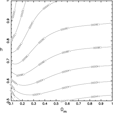
FIG. 1.: The contour of the number count of peaks in the CMB map with the sky coverage of $f_{\rm sky}=0.65$ for the expected Planck survey as a function of $\Omega_{\rm m}$ and $h$, where we have assumed the simplest flat inflationary models with $n_{s}=1$ and $\Omega_{\rm b}h^{2}=0.019$. We here employed the instrumental specifications of $\theta_{\rm fwhm}=5.5^{\prime}$ and $\sigma_{\rm pix}=4.3\times 10^{-6}$. The contour clearly shows that lowering $\omega_{\rm m}$ roughly causes an increase of the number count because of the dependence of $\omega_{\rm m}$ on amplitude and position of the acoustic peaks of $C_{l}$ in $l$-space (see text in detail).

We assume that the observational errors associated with measurements of number count of peaks with respect to a certain threshold $\nu_{\rm s}$ can be considered as a Poisson contribution estimated by $\sqrt{N_{\rm peak}(\nu_{\rm s})}$. We have verified using the numerical experiments [11] that this estimate is a good approximation. We can therefore estimate the signal to noise ratio for determinations of $\Omega_{\rm m}$ and $h$ parameters from the number count as

$$\frac{S}{N}=\frac{|N^{\rm obs}_{\rm peak}(\nu_{\rm s})-N^{\rm real}_{\rm peak}(\nu_{\rm s};\Omega_{\rm m},h)|}{\sqrt{N_{\rm peak}^{\rm obs}(\nu_{\rm s})}},$$ (7)

where the subscripts “obs” and “real” denote the observed value and theoretical prediction of the number count, respectively. Based on this consideration, Figure 2 shows contours of constant signal to noise ratio $S/N$ for determinations of $\Omega_{\rm m}$ and $h$ for the fiducial model with $\Omega_{\rm m}=0.3$ and $h=0.7$ marked with cross. The fiducial model then has $N_{\rm peak}=1.37\times 10^{5}$ and the contours or equivalently constraints on $\Omega_{m}$ and $h$ approximately scale as $\Omega h^{-4.9}$ around the point of the fiducial model. Recently, Hu et al. (2000) shows that the combined data of $C_{l}$ from BOOMERanG and MAXIMA can place the constraints on these parameters, which approximately scale as $\Omega_{\rm m}h^{3.8}$, from the measured position of fist acoustic peak around $l\approx 200$ under the assumption of a flat universe (Figure 6 in their paper). The dependence of $\Omega_{\rm m}h^{3.8}$ is also shown by two bold solid lines in Figure 2 and it clearly demonstrates that the lines almost vertically cross the $S/N$ contours of the number count. Therefore, combining both constraints allows us to accurately determine $\Omega_{\rm m}$ and $h$ or break the cosmic degeneracy by the CMB measurements alone.

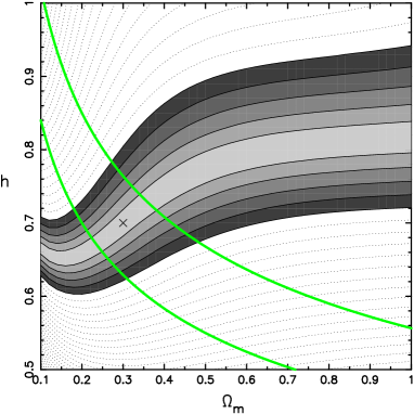
FIG. 2.: The contours of the signal to noise ratio for the measurements of the number count of peaks for the fiducial model with $\Omega_{m}=0.3$ and $h=0.7$ (marked with cross) as same models in Figure 1. The fiducial model has $N_{\rm peak}=1.37\times 10^{5}$. The contours are stepped in units of $\Delta S/N=1$ and the shaded regions denote $S/N\leq 5$ from equation (7). The two bold solid lines are an arbitrarily normalized $\Omega_{\rm m}h^{3.8}$ that represent the dependence of constraints obtained from the position of the first acoustic peak in $C_{l}$ for the flat universe (Hu et al. 2000). The lines almost vertically cross the S/N contours.

In this Letter, we propose a new potentially useful method that the number count of peaks in the CMB map can probe the cosmological parameters relatively independently of those provided by the measurements of $C_{l}$. This is because the peak statistics contains the integrated information of $C_{l}$ over $l$ space, although the number count can be derived only from $C_{l}$ based on the Gaussian theory. Thus, if we adopt the Gaussian assumption for the primordial fluctuations such as the inflationary scenarios suggest, we could extract an additional information on the underlying cosmology. As an example, we here showed that the number count of peaks can place complementary constraints on $\Omega_{\rm m}$-$h$ plane and an interesting possibility that we can determine $\Omega_{\rm m}$ by combining the constraints from $C_{l}$. This result therefore indicates that we can break the cosmic degeneracy by using the CMB data alone without invoking the other astronomical observations.

Undoubtedly, secondary anisotropies and foregrounds can mimic the peaks in the observed CMB maps. Although the most important sources are the thermal Sunyaev-Zel’dovich effect, this effect can be removed by either observing at $217$GHz or using advantage of its specific spectral property. We also have to carefully investigate the effect of Galactic foregrounds and extragalactic point sources [19] to make reliable predictions in our method, but this must be done for any measurements of statistical properties of CMB temperature map.

We thank Eiichiro Komatsu for valuable and critical comments, which considerably improved this manuscript. We are grateful to U. Seljak and M. Zaldarriaga for making available their CMBFAST code. M.T. acknowledges a support from a JSPS fellowship.

REFERENCES

- [1] P. de Bernardis, et al., Nature404, 955 (2000).
- [2] S. Hanany, et al., astro-ph/0005123, (2000).
- [3] A. E. Lange, et al., astro-ph/0005004, (2000); A. Balbi, et al., astro-ph/0005124 (2000);
- [4] M. Tegmak, and M. Zaldarriaga, to appear in Phys. Rev. Lett., astro-ph/0004393, (2000).
- [5] W. Hu, M. Fukugita, M. Zaldarriaga, and M. Tegmark, astro-ph/0006436, (2000).
- [6] M. Kamionkowski, D. N. Spergel, and N. Sugiyama, ApJLett. 426, L57 (1994); G. Jungman, M. Kamionkowski, A. Kosowsky, and D. N. Spergel, Phys. Rev. Lett.76, 1007 (1996); S. Weinberg, astro-ph/000276, (2000).
- [7] J. R. Bond, G. P. Efstathiou, and M. Tegmark, MNRAS Lett. 291, 33 (1997).
- [8] A. H. Guth, A. H., and S.-Y. Pi, Phys. Rev. Lett.49, 1110, (1985).
- [9] J. R. Bond, and G. P. Efstathiou, MNRAS226, 655 (1987).
- [10] A. F. Heavens, and R. K. Sheth, MNRAS310, 1062 (1999).
- [11] M. Takada, E. Komatsu, and T. Futamase, ApJ Lett. 533, L83 (2000); M. Takada, and T. Futamase, to appear in ApJ, astro-ph/0008377, (2000).
- [12] However, the detector noise tends to make more spurious peaks on smooth structures nearer to intrinsic peaks in the CMB sky.
- [13] S. Burles, and D. Tytler, ApJ507, 732 (1998).
- [14] U. Seljak, and M. Zaldarriaga, ApJ469, 437 (1996).
- [15] L. Knox, Phys. Rev. D52, 4307 (1995); M. P. Hobson, and J. Magueijo, MNRAS283, 1133 (1996).
- [16] E. F. Bunn, and M. White, ApJ480, 6 (1997).
- [17] A. Sandage, ApJ133, 355 (1961); T. Totani, and Y. Yoshii, ApJ540, 81 (2000).
- [18] W. Hu, and N. Sugiyama, Phys. Rev. D51, 2599 (1995); W. Hu, and N. Sugiyama, ApJ471, 542, (1996).
- [19] See, e.g., M. Tegmark, D. J. Eisenstein, W. Hu, and A. de Oliveira-Costa, ApJ530, 133 (2000).