Power spectrum of the polarized diffuse Galactic radio emission

We have analyzed the available polarization surveys of the Galactic emission to estimate to what extent it may be a serious hindrance to forthcoming experiments aimed at detecting the polarized component of Cosmic Microwave Background (CMB) anisotropies. Regions were identified for which independent data consistently indicate that Faraday depolarization may be small. The power spectrum of the polarized emission, in terms of antenna temperature, was found to be described by $C^{P}_{\ell}\simeq(1.2\pm 0.8)\cdot 10^{-9}\cdot(\ell/450)^{-1.8\pm 0.3}\cdot(\nu/2.4{\rm GHz})^{-5.8}$ K², from arcminute to degree scales. Data on larger angular scales ($\ell\leq 100$) indicate a steeper slope $\sim\ell^{-3}$. We conclude that polarized Galactic emission is unlikely to be a serious limitation to CMB polarization measurements at the highest frequencies of the MAP and Planck-LFI instruments, at least for $\ell\geq 50$ and standard cosmological models. The weak correlation between polarization and total power and the low polarization degree of radio emission close to the Galactic plane is interpreted as due to large contributions to the observed intensity from unpolarized sources, primarily strong Hii regions, concentrated on the Galactic plane. Thus estimates of the power spectrum of total intensity at low Galactic latitudes are not representative of the spatial distribution of Galactic emission far from the plane. Both total power and polarized emissions show highly significant deviations from a Gaussian distribution.

1 Introduction

Several ongoing or planned experiments (see Staggs et al.1999 for a recent review) are designed to reach the sensitivities required to measure the expected linear polarization of the Cosmic Microwave Background (CMB).

The forthcoming space missions Planck and MAP, aimed at obtaining full sky high sensitivity and high resolution maps (FWHM of about $56^{\prime}$, $41^{\prime}$, $28^{\prime}$, $21^{\prime}$, and $13^{\prime}$ for MAP channels at 22, 30, 40, 60, and 90 GHz, respectively; of $33^{\prime}$, $23^{\prime}$, $14^{\prime}$, $10^{\prime}$ for Planck “radiometric” channels at 30, 44, 70, and 100 GHz; of $10^{\prime}.7$, $8^{\prime}$, $5^{\prime}.5$, $5^{\prime}$, $5^{\prime}$, $5^{\prime}$ for Planck “bolometric” channels at 100, 143, 217, 353, 545, and 857 GHz, respectively) of CMB anisotropies will also probe the CMB polarization fluctuations (Mandolesi et al. 1998; Puget et al. 1998; MAP webpage: http://map.gsfc.nasa.gov/; Planck webpage: http://astro.estec.esa.nl/SA-general/Projects/-
Planck/). We recall that the CMB radiation brightness peaks at about 160 GHz.

The current design of instruments for the Planck mission (the third Medium-size mission of ESA’s Horizon 2000 Scientific Programme) provides good sensitivity to polarization at all LFI (Low Frequency Instrument) frequencies (30–100 GHz) as well as at three HFI (High Frequency Instrument) frequencies (143, 217 and 545 GHz). The NASA’s MIDEX class mission MAP has also polarization sensitivity in all channels.

While there is a very strong scientific case for CMB polarization measurements (cf., e.g., Zaldarriaga 1998 and references therein), they are very challenging both because of the weakness of the signal and because of the contamination by foregrounds that may be more polarized than the CMB.

Our knowledge of polarized foreground components is very meager (see Davies & Wilkinson 1999 for a recent review). In this paper we present a preliminary investigation of the power spectrum of the polarized Galactic synchrotron emission, the likely dominant foreground contribution at microwave frequencies where CMB is dominating, at least at intermediate to large angular scales (Tegmark et al. 2000). When this work was approaching completion we learned that a similar analysis was carried out by Tucci et al. (2000). We improve on their results by taking into account, in addition to the Parkes survey (Duncan et al. 1995, 1997; hereafter D97) discussed by them, the more recent Effelsberg surveys at 2.7 GHz (Duncan et al. 1999; D99) and at 1.4 GHz, covering areas up to $\pm 20^{\circ}$ of Galactic latitude (Uyaniker et al. 1998, 1999; U99), as well as the Leiden surveys (Brouw & Spoelstra 1976; BS76). We also discuss in some detail the effect of the emission from Hii regions in the Galactic plane and of the Faraday depolarization.

The Galactic polarized thermal dust emission has been modelled by Prunet et al.  (1998); based on their results, we may expect that fluctuations of polarized dust emission prevail over those of polarized synchrotron emission above 100–150 GHz. De Zotti et al. (1999) discussed polarization fluctuations due to extragalactic sources. Additional polarized contributions are expected from magneto-dipole emission or rotational emission of dust grains (Draine & Lazarian 1999; Lazarian & Draine 2000) and scattered free-free emission (Keating et al. 1998). A multifrequency Wiener filtering method to detect CMB polarization in the presence of polarized foregrounds has been worked out by Bouchet et al. (1999).

2 Polarization surveys

Linear polarization observations extending up to high Galactic latitudes and carried out at several frequencies, from 408 to 1411 MHz, have been presented by BS76 (Leiden surveys). The half power beamwidths varied with increasing frequency from $2.3^{\circ}$ to $0.6^{\circ}$. Unfortunately these and the other surveys discussed by Spoelstra (1984) are undersampled so that proper smoothing to the largest beamwidth, as required to combine data at different frequencies, is not possible. Thus, estimates of differential polarization and differential Faraday rotation across the beam cannot be made. We have limited our analysis of these data to patches of the sky with better than average sampling.

High resolution polarimetric surveys of strips around the Galactic plane at 2.4 and 2.695 GHz, respectively, have recently been published by D97 and D99. U99 carried out a surface brightness and polarization survey of four fields at medium Galactic latitudes (up to $b=20^{\circ}$), at 1.4 GHz. These data, together with details about the instrumental capabilities, can be found on the WEB site http://www.mpifr-bonn.mpg.de/survey.html.

D97 covered $127^{\circ}$ of Galactic longitude ($238^{\circ}<{\rm l}<5^{\circ}$) out to at least $b=\pm 5^{\circ}$ (for $340^{\circ}<{\rm l}<5^{\circ}$ the survey extends to $b=+7^{\circ}$, for $340^{\circ}<{\rm l}<352^{\circ}$ to $b=-7^{\circ}$, and for $240^{\circ}<{\rm l}<270^{\circ}$ to $b=-8^{\circ}$) with an angular resolution of $10.4^{\prime}$. The surveyed area amounts to $\simeq 1413$ square degrees. The nominal rms noise in total power is 17 mJy/beam area (8 mK), and 11 mJy/beam area (5.3 mK) for polarization; however a lower rms noise of 11 mJy/beam area (5.3 mK) for total intensity and 6 mJy/beam area (2.9 mK) for polarization has been achieved over $\simeq 43\%$ of the total area. The center frequency is 2.417 GHz and the bandwidth about 145 MHz. Values of the Stokes $Q$ and $U$ parameters and of the total power are given every $4^{\prime}$ on a rectangular grid, in units of mJy/beam area; the conversion factor to brightness temperature is $1\,\hbox{mJy/beam area}=0.48\,$mK (Duncan, private communication).

Polarimetric data from the Effelsberg 2.695 GHz survey with half-power beamwidth of $4.3^{\prime}$ in the first Galactic quadrant were reported by D99. Maps at a resolution of $5.1^{\prime}$ of the Stokes $Q$ and $U$ emission components, covering the region $74^{\circ}\geq{\rm l}\geq 4^{\circ}.9$, $|b|\leq 5^{\circ}$, with a rms noise of 2.5 mJy/beam area (corresponding to 9 mK) were constructed.

Of particular interest for our purposes is the continuum and polarization survey at 1.4 GHz, also carried out with the Effelsberg 100-m telescope, at medium Galactic latitudes (up to $b=\pm 20^{\circ}$). Four areas were observed (with the one in the Cygnus region split in two parts), totaling about 1050 sq. deg.: one in the first Galactic quadrant ($45^{\circ}\geq{\rm l}\geq 55^{\circ}$, $4^{\circ}\geq b\geq 20^{\circ}$); the northern ($65^{\circ}\geq{\rm l}\geq 95^{\circ}$, $5^{\circ}\geq b\geq 15^{\circ}$) and the southern ($70^{\circ}\geq{\rm l}\geq 100^{\circ}$, $-15^{\circ}\geq b\geq-5^{\circ}$) parts of the Cygnus region; the highly polarized “fan region” ($140^{\circ}\geq{\rm l}\geq 153^{\circ}$, $3.5^{\circ}\geq b\geq 10^{\circ}$); the anticentre region ($190^{\circ}\geq{\rm l}\geq 210^{\circ}$, $3.8^{\circ}\geq b\geq 15^{\circ}$). The rms noise is about 15 mK (about 7 mJy/beam area) for total intensity and about 8 mK in linear polarization; the angular resolution is $9.35^{\prime}$.

From the MPIfR survey Web-site mentioned above it is possible to download both “background” and “source” total power maps, which correspond to large and small-scale components of the total intensity, as well as polarization maps. To derive the total Galactic emission we have subtracted from the sum of “background” and “source” maps the isotropic component due to the CMB and to the contribution of unresolved extragalactic sources. We have adopted, for this component, $T_{A,{\rm isot}}=2.9\,$K.

Figure 1: Total versus polarized intensity in the $300^{\circ}\leq{\rm l}\leq 320^{\circ}$ region from the D97 data at 2.4 GHz, showing no correlation at all.

3 Analysis of survey data

3.1 Depolarization

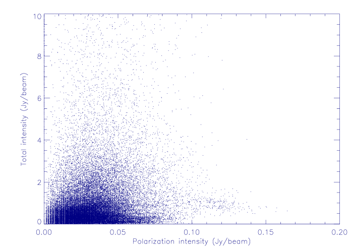
A comparison of total power and polarized emission maps (Duncan et al. 1995, 1997; Uyaniker et al. 1998, 1999) shows little correlation. While the total intensity clearly peaks on the Galactic Plane (apart from a number of spurs and loops extending to high Galactic latitude), the polarized intensity is much more uniformly distributed. Also, many sources which are very intense in total power are not seen in polarized emission and, conversely, bright regions of extended polarization do not appear to be connected with sources of total-power emission (D97, U99). This is seen in Fig. 1, showing, as an example, the polarization intensity $\sqrt{Q^{2}+U^{2}}$ versus the total intensity for the Parkes survey data in the region $300^{\circ}\leq{\rm l}\leq 320^{\circ}$ and $|b|\leq 5^{\circ}$.

Two main factors may contribute to this situation. On one side, many bright structures on the Galactic plane are (unpolarized) Hii regions and significant thermal radio emission is also expected between and above bright Hii regions in our Galaxy: Duncan et al. (1995) estimate a thermal flux level of the order of 100 mJy per beam area at 2.4 GHz, comparable to the level of the radio continuum often observed near these regions. The large thermal contributions to the Galactic emission, which are concentrated close to the Galactic plane, obviously make it very unlikely that the total intensity power spectra for these regions can be representative of the synchrotron power spectra at high Galactic latitudes.

On the other side, differential Faraday rotation or variations of the magnetic field orientation may strongly depolarize the emission from distant regions of the Galaxy (Burn 1966, Gardner & Whiteoak 1966; for a recent, detailed discussion of depolarization mechanisms, see Sokoloff et al. 1998) so that only the polarized emission of relatively local origin can be observed. The two factors may act together: variations in the density of thermally emitting electrons may lead to a large enough differential Faraday rotation to produce substantial depolarization; in addition, the magnetic field may be tangled by turbulent motions of the ionized gas, leading to further depolarization.

The Faraday rotation of the polarization position angle of a linearly polarized wave at a wavelength $\lambda$ traversing an ionized medium with electron density $n_{e}$ and a regular magnetic field ${\bf B}$ is given by:

$$\phi(\lambda)=\hbox{RM}\lambda^{2}\ \hbox{rad},$$ (1)

where the rotation measure RM is the line-of-sight integral

RM $$= {e^{3}\over 2\pi m_{e}^{2}c^{4}}\int n_{e}{\bf B}\cdot d{\bf l}=$$ (2)

$$= 810\int n_{e}(\hbox{cm}^{-3})B_{\parallel}(\mu\hbox{G})\cdot dl(\hbox{kpc})\ \hbox{rad}\,\hbox{m}^{-2}.$$

Since $\phi$ scales as $\nu^{-2}$, the Faraday rotation is likely irrelevant at microwaves, where MAP and Planck instruments will operate, while it may strongly distort the power spectrum of polarized emission at the decimetric wavelengths considered here, on one side by wiping out polarized emission from far regions (due to differential rotation within the beamwidth or the bandwidth of observations) and, on the other side, introducing structure on a variety of scales (larger than the beamwidth) due to fluctuations in the thermal electron density distribution and/or magnetic field variations (in strength and/or direction) along the line of sight.

If the synchrotron emission arises throughout the depth of the Faraday rotating medium, the polarization degree is reduced from the intrinsic value $P_{0}$ to (Burn 1966):

$$P(\lambda)=P_{0}{\sin\phi\over\phi}\ .$$ (3)

For $\phi=1\,$rad, corresponding to $\hbox{RM}(\hbox{rad}\,\hbox{m}^{-2})=21.8$, 64.1, and 80.8 for $\nu=1.4$, 2.4, and $2.7\,$GHz, respectively, the depolarization amounts to about 16%. Spoelstra (1984), from his analysis of multifrequency data on linear polarization, found that the distribution of RM over the sky shows a complex pattern with typical values (in the region covered by Leiden surveys) of $8\,\hbox{rad}\,\hbox{m}^{-2}$. As pointed out by the referee, however, Spoelstra’s estimates of RMs are actually lower limits because there may be field reversals along the line of sight, his surveys have different resolutions and differential Faraday depolarization can lead to small observed RMs (see Sokoloff et al. 1998). Accurate estimates of the amount of depolarization were obtained, for the Leiden survey at 820 MHz, by Berkhuijsen (1971) who determined the percentage polarization using the absolutely calibrated total power survey at that frequency. The polarization percentages given in that work should be scaled by 0.8 (Berkhuijsen 1975) and are not corrected for the thermal contribution from ionized gas, which decreases the polarization degree.

The implied RMs are relatively small over the surveyed area, particularly at high Galactic latitudes.

The Galactic RM distribution is also probed by Faraday rotation measurements towards pulsars and extragalactic radio sources. Since pulsar distances can often be independently derived, pulsar data also provide information on the variation of RM along the line of sight; also, they appear to have no intrinsic Faraday rotation and hence their observed RM arises entirely along the path to the observer. Extragalactic sources can provide information on the Galactic medium out to large distances, beyond those where pulsars are found; on the other hand, extragalactic sources may have their own Faraday rotation which adds to the Galactic contribution.

A catalogue of known pulsars, including values of RM, has been published by Taylor et al. (1993); an updated version is available on the WEB (see Appendix of Taylor et al. 1993). Additional RMs have been published by Manchester & Johnston (1995), Navarro et al. (1997) and Han et al. (1999); on the whole, we have collected RMs for 318 pulsars.

Rotation measures for 674 extragalactic sources have been catalogued by Broten et al. (1988). Additional RMs have been published by Clegg et al.  (1992).

An analysis of the RM of pulsars and extragalactic sources located in the sky areas covered by polarization surveys considered here reveals a number of regions where RMs can produce only a small Faraday depolarization ($\phi\leq 1\,$rad).

One of these is the area $140^{\circ}\leq{\rm l}\leq 153^{\circ}$, $3^{\circ}.7\leq b\leq 10^{\circ}$, surveyed by U99. This partly covers the highly polarized region referred to as the “fan region” where the rotation measures have long been known to be small (Bingham & Shakeshaft 1967) and the magnetic field direction has to be basically perpendicular to the line of sight.

Figure 2: Distributions of polarized intensities for the U99 regions centered at ${\rm l}=50^{\circ}$ (solid line), $80^{\circ}$ ($b\geq 8^{\circ}$; short dashes), $146^{\circ}.4$ (dotted line), and $200^{\circ}$ (long dashes).

Figure 3: Distributions of total intensities (isotropic component subtracted, see text) for the U99 regions centered at ${\rm l}=50^{\circ}$ (solid line), $80^{\circ}$ ($b\geq 8^{\circ}$; short dashes), $146^{\circ}.4$ (dotted line), and $200^{\circ}$ (long dashes). The maps used for this analysis do not include $\geq 5\sigma$ unresolved discrete sources; addition of these enhances the high intensity tails.

Table 1: Polarization degrees of non-thermal emission at 1.4 GHz for several U99 fields (Berkhuijsen, private communication).

l (deg)	b (deg)	$P(\%)$
151.5	$+6$	20
146	$+7$	4
50	$+10$	3
78	$+10$	19
86	$+10$	12
80	$-10$	9
92	$-10$	10

Berkhuijsen (private communication) has estimated the observed polarization degree of non-thermal emission for several U99 fields discussed in this paper (see Table LABEL:Berk). The total synchrotron emission was derived subtracting from the observed intensities the contributions from extragalactic radio sources and the CMB (3 K at 1.4 GHz) and from thermal emission. The fraction of thermal emission at 1.4 GHz, $f_{\rm therm}$, was obtained from

$$f_{\rm therm}={1-(\nu_{1}/\nu_{2})^{s-\gamma}\over 1-(\nu_{1}/\nu_{2})^{t-\gamma}}$$ (4)

where $s$ is the observed spectral index (in terms of antenna temperature: $T_{A}\propto\nu^{-s}$) between $\nu_{1}=1420\,$MHz and $\nu_{2}=408\,$MHz taken, for each field, from Reich & Reich (1988), and $\gamma=2.9$, $t=2.1$ are the spectral indices of non-thermal and thermal emission, respectively. The highest polarization degree of non-thermal emission found in these fields is about 20%, well below the theoretical maximum corresponding to a uniform magnetic field (Ginzburg & Syrovatskii 1965):

$$\Pi={3-3\gamma\over 1-3\gamma}\ ,$$ (5)

which, for $\gamma=2.9$, is $\Pi=74\%$. To depolarize to the observed level with differential Faraday rotation, $\hbox{RM}>53\leavevmode\nobreak\ \hbox{rad}\,\hbox{m}^{-2}$ would be required, much higher than the RMs directly measured. Thus, other depolarization mechanisms must be operating.

Table 2: Moments of the distributions of total and polarized intensities.

	mean (mK)		$\sigma$ (mK)		skewness		kurtosis
	int	pol	int	pol	int	pol	int	pol
Uyaniker ${\rm l}=50^{\circ}$	2480	155	550	70	$0.9\pm 0.5$	$1.3\pm 0.1$	$5.5\pm 3.5$	$3.2\pm 0.3$
no sources	2360		440		$0.051\pm 0.007$		$-0.89\pm 0.02$
Uyaniker ${\rm l}=80^{\circ}$∗	1640	125	310	60	$19\pm 12$	$0.54\pm 0.05$	$74\pm 36$	$1.0\pm 0.1$
no sources	1610		270		$2.0\pm 0.06$		$2.0\pm 0.1$
Uyaniker ${\rm l}=146^{\circ}.4$	1840	110	190	65	$28\pm 7$	$0.43\pm 0.04$	$58\pm 10$	$-0.07\pm 0.08$
no sources	1740		50		$0.67\pm 0.07$		$1.0\pm 0.1$
Uyaniker ${\rm l}=200^{\circ}$	1270	70	230	40	$23\pm 11$	$0.36\pm 0.03$	$82\pm 22$	$-0.05\pm 0.1$
no sources	1200		140		$0.23\pm 0.01$		$-0.94\pm 0.03$
D97 $240^{\circ}\leq{\rm l}\leq 260^{\circ}$	161	13	110	9	$60\pm 40$	$0.26\pm 0.02$	$210\pm 80$	$0.08\pm 0.07$
no sources	129		70		$0.004\pm 0.003$		$-0.15\pm 0.03$
D97 $280^{\circ}\leq{\rm l}\leq 300^{\circ}$	425	106	1741	33	$340\pm 40$	$0.98\pm 0.05$	$470\pm 60$	$1.0\pm 0.1$
no sources	192		227		$1.41\pm 0.04$		$0.53\pm 0.07$
D97 $300^{\circ}\leq{\rm l}\leq 320^{\circ}$	577	15	930	15	$90\pm 20$	$0.88\pm 0.05$	$200\pm 30$	$0.7\pm 0.2$
no sources	423		404		$0.59\pm 0.02$		$-0.22\pm 0.04$
D99 $20^{\circ}\leq{\rm l}\leq 30^{\circ}$	317	32	907	20	$130\pm 40$	$1.3\pm 0.3$	$270\pm 70$	$4\pm 2$
D99 $55^{\circ}\leq{\rm l}\leq 65^{\circ}$	72	32	18	11	$1500\pm 300$	$0.49\pm 0.03$	$2400\pm 300$	$0.6\pm 0.1$

^∗ Analysis limited to the region $8^{\circ}\leq b\leq 15^{\circ}$

Figure 4: Global skewness of the total (upper, solid line) and polarized emissions (dashed) for the D97 survey compared with the rms error on the skewness derived from Monte Carlo simulations for a $10^{\circ}\times 10^{\circ}$ patch (grid $4^{\prime}\times 4^{\prime}$ as default in the D97 data) assuming the same power spectrum for the signals but a Gaussian distribution (straight dotted line at the bottom).

3.2 Distribution of total intensity and polarization signals

All maps were put onto the same $12^{\prime}\times 12^{\prime}$ grid. Although these cells are not totally independent (the telescope beamwidth is $9.35^{\prime}$), we do not need to worry much about that since the derived power spectrum is affected only on small scales, where fluctuations due to point sources dominate anyway (De Zotti et al. 1999).

It is clear from Figs. 2 and 3 that the distributions of both total and polarized emissions are distinctly non-Gaussian. The statistical significance of this visual impression can be quantified by computing the moments of order $>2$:

$$\mu_{\rm i}={\sum_{j=1}^{n}(S_{\rm j}-\bar{S})^{\rm i}\over n-1}\ ,$$ (6)

where $S_{\rm j}$ is the measured signal (polarized or unpolarized intensity in the j-th cell) and $\bar{S}$ is its mean over the considered sky region.

It is convenient to define the dimensionless quantities $\beta_{1}=\mu_{3}^{2}/\mu_{2}^{3}$, $\beta_{2}=\mu_{4}/\mu_{2}^{2}$, $\beta_{3}=\mu_{3}\mu_{5}/\mu_{2}^{4}$, $\beta_{4}=\mu_{6}/\mu_{2}^{3}$, $\beta_{5}=\mu_{7}\mu_{3}/\mu_{2}^{5}$, $\beta_{6}=\mu_{8}/\mu_{2}^{4}$.

Usual definitions of skewness and of kurtosis are ${\rm skewn}=\sqrt{\beta_{1}}$ and ${\rm kurt}=\beta_{2}-3$, which vanish for a Gaussian distribution. The probable errors of $\beta_{1}$ and $\beta_{2}$ are given by (Pearson 1924):

$$\Delta\beta_{1} = 0.6745(\beta_{1}/n)^{1/2}\cdot$$ (7)

$$\cdot {\left(4\beta_{4}-24\beta_{2}+36+9\beta_{1}\beta_{2}-12\beta_{3}+35\beta_{1}\right)^{1/2}}$$

$$\Delta\beta_{2} = 0.6745n^{-1/2}\cdot$$

$$\cdot(\beta_{6} - 4\beta_{2}\beta_{4}+4\beta_{2}^{3}-\beta_{2}^{2}+16\beta_{1}\beta_{2}-8\beta_{3}+16\beta_{1})^{1/2}.$$ (8)

The values of skewness and kurtosis for the regions we have analyzed, and their errors, are given in Table LABEL:moments, together with the mean total and polarization intensities and their standard deviations $\sigma$. Note that, for the U99 area centered at ${\rm l}=80^{\circ}$, we have limited our analysis to the region above $b=8^{\circ}$ to avoid the relatively large hole in the map at lower Galactic latitudes.

The deviations from the Gaussian value (zero) of skewness and/or kurtosis are in general highly significant, both for total and for polarized emissions. This conclusion is strengthened by the Monte Carlo simulations reported in Fig. 4 for $10^{\circ}\times 10^{\circ}$ patches (grid $4^{\prime}\times 4^{\prime}$ as default in the D97 data), showing that the skewness differs from $0$ at a $\,\lower 2.0pt\hbox{${>\atop\hbox{\raise 4.0pt\hbox{$\sim$}}}$}\,10\sigma$ level in the case of polarization and even more for total intensity. This may be a difficulty for methods involving Wiener filtering of the data to remove foreground contributions to CMB maps (Bouchet et al. 1999) since a Gaussian approximation for the distribution of foreground signals is assumed. On the other hand, Independent Component Analysis algorithms (Baccigalupi et al. 2000) require that all independent components contributing to the observed maps, except, at most, one have non-Gaussian distributions.

Figure 5: Reconstructed power spectrum of CMB temperature fluctuations from a simulated $10^{\circ}\times 10^{\circ}$ patch (solid line) compared with the theoretical spectrum predicted by a standard CDM model, averaged over the whole sky (dashed line).

4 Intensity and polarization power spectra

It is currently standard practice to adopt as a statistical measure of the temperature pattern on the celestial sphere, the power spectrum of temperature fluctuations, $C_{\ell}$, which turned out to be of fundamental importance in studies of CMB anisotropies.

The $C_{\ell}$’s are defined as follows. The spherical harmonic expansion of the sky signal $s$ writes:

$$s(\hat{n})=\sum_{\ell m}a_{\ell m}Y_{\ell}^{m}(\hat{n})\ ,$$ (9)

where $a_{\ell m}$ are the expansion coefficients, $\hat{n}$ is the unit vector in the direction $(\vartheta,\phi)$, and the spherical harmonic $Y_{\ell}^{m}$ is related to the Legendre function, $P_{\ell}^{|m|}$, of degree $\ell$ and order $m$ ($|m|\leq\ell$) by $Y_{\ell}^{m}(\vartheta,\phi)=c_{\ell}^{m}P_{\ell}^{|m|}(\cos\vartheta)\exp(im\phi)$; the coefficients $c_{\ell}^{m}$ normalize the spherical harmonics to $\int d\Omega Y_{\ell}^{m}Y_{\ell^{\prime}}^{m^{\prime}}=\delta_{\ell\ell^{\prime}}\delta{mm^{\prime}}$. The correlation function $C(\theta)=<s(\hat{n})s(\hat{n}^{\prime})>_{\hat{n}\cdot{\hat{n}^{\prime}}=\cos\theta}$ can be expanded into Legendre polynomials, with coefficients given by

$$C_{\ell}={1\over 2\ell+1}\sum_{m=-\ell}^{\ell}|a_{\ell m}|^{2}\ .$$ (10)

The multipole $\ell$ corresponds to the angular scale

$$\theta\simeq 180/\ell\ {\rm degrees}\ .$$ (11)

We have projected each sky patch onto a null signal sphere and computed the power spectrum using of the HEALPix tools (Górski et al. 1998). The coefficients were renormalized by simply dividing by the fractional coverage of the sky.

Note that the use of spherical harmonics is not strictly necessary, given that we are dealing with limited areas of the sky. In fact, for the common data sets, our results agree with those by Tucci et al. (2000) who resorted to a standard Fourier analysis technique. We preferred, however, to stick to the spherical harmonic analysis to be used for the all sky MAP and Planck data.

We have tested our method using a simulation of a purely cosmological signal. We have generated an all sky map of the CMB temperature distribution as predicted by a standard model for a Cold Dark Matter (CDM) dominated universe, at a resolution of about $3.5^{\prime}$. We have then applied our algorithm to a randomly chosen $10^{\circ}\times 10^{\circ}$ patch. In Fig. 5 we show the recovered power spectrum for the patch compared with the theoretical one (which is, of course, an all-sky average). The reconstructed spectrum oscillates around the theoretical one, due to the sample variance, i.e.to the very limited sampling of a random, all sky process. However, the main features of the spectrum are recovered.

Linear polarization is described by the Stokes parameters $Q$ and $U$, from which the total polarization intensity $PI=\sqrt{Q^{2}+U^{2}}$ and the polarization angle $\phi_{P}=\arctan{(U/Q)}$, can be derived. $PI$ is a scalar quantity that can be expanded into spherical harmonics [Eq. (9)]; its power spectrum coefficients $C_{\ell}^{P}$ can be computed as in Eq. (10).

In order to derive the true power spectrum coefficients from the measured ones, $C_{\ell}^{\rm map}$, we must allow for the contribution of instrumental noise and for the effect of the detector response function $b(\ell)$:

$$C_{\ell}={C_{\ell}^{\rm map}-C_{\ell}^{\rm noise}\over W(\ell)}\ ,\ \ W(\ell)=b(\ell)^{2}\ .$$ (12)

The beam response for each multipole is modelled by

$$b(\ell)=\exp[-\ell(\ell+1)\sigma_{\rm beam}^{2}/2]\ .$$ (13)

where $\sigma_{\rm beam}={\rm FWHM}/(2\sqrt{2\ln 2})$ and FWHM is the full width at half maximum, in radians. In the case of D97, the beam is slightly elliptical and Eq. (13) has been modified accordingly.

The instrumental noise has an approximately flat power spectrum:

$$C_{\ell}^{\rm noise}=4\pi{\sigma^{2}_{\rm noise}\over N_{\rm pixels}}\ .$$ (14)

For the surveys of D97, D99 and U99 we have adopted the values of the instrumental noise given by the authors (taking into account the different sensitivities reached by D97 in different regions). In the case of the BS76 data, we found it convenient to treat the noise as a parameter to be determined (see subsection 4.2).

We have analyzed $10^{\circ}\times 10^{\circ}$ patches of the surveys by D97, D99 and U99. Correspondingly, the minimum value of $\ell$ for which the power spectrum can be estimated is $\simeq 100$, corresponding to an angular scale of about $2^{\circ}$: as the angular scale approaches the size of the patch, the effects of poor sampling become unacceptably large. Information on larger angular scales is provided by the BS76 data. The maximum value of $\ell$ is determined by the angular resolution of the survey; we have $\ell_{\rm max}\simeq 800$.

Figure 6: Polarization (upper panels) and total intensity (lower panels) angular power spectra for the D97 region $360^{\circ}\geq{\rm l}\geq 320^{\circ}$. The panels correspond to $10^{\circ}$ intervals in longitude, with l decreasing from left to right. The dashed lines represent power law fits.

Figure 7: Polarization (upper panels) and total intensity (lower panels) angular power spectra for the D97 region $320^{\circ}\geq{\rm l}\geq 280^{\circ}$. The panels correspond to $10^{\circ}$ intervals in longitude, with l decreasing from left to right. The dashed lines represent power law fits.

Figure 8: Polarization (upper panels) and total intensity (lower panels) angular power spectra for the D97 region $280^{\circ}\geq{\rm l}\geq 240^{\circ}$. The panels correspond to $10^{\circ}$ intervals in longitude, with l decreasing from left to right. The dashed lines represent power law fits.

4.1 Low and medium Galactic latitudes

We have focused our analysis on the low RM regions of the D97, D99, and U99 surveys. As detailed in the following, we find that these regions do possess remarkably similar polarization power spectra.

Following Maino et al. (1999) we divided the D97 data in twelve $10^{\circ}\times 10^{\circ}$ subpatches, and we evaluated the power spectrum of both total intensity and polarization for each patch, over the range $100\leq\ell\leq 800$. The results are plotted in Figs. 6–8. In each panel, the dashed line shows a power law fit ($C_{\ell}=\alpha\cdot\ell^{\beta}$).

Figure 9: Total (upper panel) and polarized intensity fluctuations in the area surveyed by D97.

Figure 10: Power spectrum for total intensity (dotted line) and polarization (dashed line) in the $240^{\circ}\leq{\rm l}\leq 250^{\circ}$ D97 region. The solid line shows the power spectrum coefficients $C_{\ell}$ of total intensity before (dotted line) and after (solid line) removing the most prominent sources as described in the text, in comparison with polarization (dashed line).

Table 3: Bright Hii regions between ${\rm l}=300^{\circ}$ and ${\rm l}=320^{\circ}$.

l (deg.)	$b$ (deg.)	$S_{2.7{\rm GHz}}\,$(Jy)	Size (′)
305.1	0.1	16.3	5
305.2	0.0	62.2	7
305.2	0.2	50.1	4.8
305.4	0.2	62.2	3.5
305.6	0.0	37.6	8
307.6	-0.3	12.2	4.2
308.6	0.6	17.8	7.8
308.7	0.1	12.0	–
308.7	0.6	21.0	–
309.6	1.7	51.0	7.5
310.8	-0.4	16.6	10.9
311.9	0.1	12.9	4
311.9	0.2	11.5	4
312.3	-0.3	10.0	–
316.3	0.0	12.0	–
316.8	-0.1	43.2	2.7
317.0	0.3	15.0	7
318.0	-0.8	11.0	10.8
319.2	-0.4	12.4	5.9
320.2	0.8	11.0	1.8
320.3	-1.4	12.0	–
320.3	-1.0	23.0	–
320.4	-1.1	17.5	6
320.4	-1.0	13.0	5.6

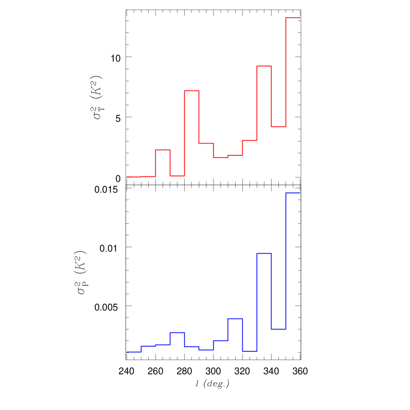
Fig. 9 shows the fluctuations around the mean of both total and polarized intensities for the D97 survey, as a function of the angular distance from the Galactic center, for regions $10^{\circ}$ wide in longitude. It may be noted that polarization and total intensity fluctuations are correlated only near the Galactic center. The intensity peaks are associated to the most prominent Galactic sources, i.e. the Galactic center and the Vela Supernova remnant ($260^{\circ}\leq{\rm l}\leq 270^{\circ}$). For polarization, the signals at $320^{\circ}\leq{\rm l}\leq 360^{\circ}$ are due to features appearing near the Galactic center such as the polarization “plume” (Duncan et al. 1998), while away from the Galactic center, at ${\rm l}\leq 320^{\circ}$, only the supernova remnant produces peaks both in total and in polarized intensity.

Also, and most important, this figure shows that the total intensity fluctuations are higher by 2 or 3 orders of magnitude than the polarization ones, implying a polarization degree much lower than the maximum expected for undepolarized synchrotron emission.

In fact, most of the observed intensity close to the Galactic plane appears to come from bright Hii regions. For example, the region between ${\rm l}=300^{\circ}$ and ${\rm l}=320^{\circ}$ contains 95 catalogued bright Hii regions (Paladini et al. 2000); the brightest ones are listed in Table 3 with their flux density at 2.7 GHz and their angular sizes which are typically in the range $2^{\prime}$–$10^{\prime}$. It is easily checked that these sources account for most, if not all, of the total intensity reported by D97. The intensity fluctuations due to them can be roughly estimated to be:

$$\sigma_{HII}^{2}\simeq{\sum_{i}S_{i}^{2}\over N_{\rm pixels}}\ ,$$ (15)

where $S_{i}$ is the flux of the $i-th$ Hii region in the catalogue, scaled to the D97 resolution and to 2.4 GHz by assuming a spectral index of 0.1 ($S_{\nu}\propto\nu^{-0.1}$), appropriate for the free-free emission. This yields $\sigma_{H{\sc ii}}\simeq 1\ {\rm Jy/beam}$, close to the value of 1.4 Jy/beam that we obtain from the D97 data.

The free-free emission from Hii regions is not polarized, but Thomson scattering by the electrons in the Hii region itself may polarize the radiation tangentially to the edges of the cloud structure at a maximum level of about 10% for an optically thick cloud (Keating et al. 1998).

Another indication that sources contributing most of the intensity in the area surveyed by D97 are unpolarized is obtained by removing the highest intensity peaks and replacing their signal with the median value in an annulus around them. As shown by Fig. 10, this has the effect of strongly decreasing the amplitude of the total intensity power spectrum, particularly at intermediate and small angular scales, making its shape quite similar to that of the polarization power spectrum. Also, the polarization degree becomes $\simeq 0.3$, consistent with moderately depolarized synchrotron emission.

Table 4: Power spectrum parameters of total intensity for the D97 survey. The first column gives the Galactic longitude of the patch center.

l (deg.)	$\alpha\ ({\rm K}^{2})$	$\beta$	$\Delta\alpha\ ({\rm K}^{2})$	$\Delta\beta$
355	3.1	-1.66	0.1	6$\cdot 10^{-3}$
345	6.8$\cdot 10^{-2}$	-1.32	4$\cdot 10^{-3}$	1$\cdot 10^{-2}$
335	7.3	-2.04	0.7	2$\cdot 10^{-2}$
325	0.21	-1.63	2$\cdot 10^{-2}$	2$\cdot 10^{-2}$
315	1.0	-2.06	0.2	3$\cdot 10^{-2}$
305	0.39	-1.67	2$\cdot 10^{-2}$	1$\cdot 10^{-2}$
295	0.16	-1.37	1$\cdot 10^{-2}$	1$\cdot 10^{-2}$
285	11.6	-1.94	0.7	1$\cdot 10^{-2}$
275	1.1$\cdot 10^{-4}$	-0.76	5$\cdot 10^{-6}$	7$\cdot 10^{-3}$
265	4.2$\cdot 10^{-2}$	-1.19	2$\cdot 10^{-3}$	7$\cdot 10^{-3}$
255	7.6$\cdot 10^{-3}$	-1.87	8$\cdot 10^{-4}$	2$\cdot 10^{-2}$
245	5.3$\cdot 10^{-5}$	-0.98	4$\cdot 10^{-6}$	1$\cdot 10^{-2}$

Table 5: Power spectrum parameters of polarized intensity for the D97 survey. The first column gives the Galactic longitude of the patch center.

l (deg.)	$\alpha\ ({\rm K}^{2})$	$\beta$	$\Delta\alpha\ ({\rm K}^{2})$	$\Delta\beta$
355	7.5$\cdot 10^{-5}$	-1.49	7$\cdot 10^{-6}$	2$\cdot 10^{-2}$
345	2.1$\cdot 10^{-5}$	-1.47	2$\cdot 10^{-6}$	2$\cdot 10^{-2}$
335	4.2$\cdot 10^{-5}$	-1.44	4$\cdot 10^{-6}$	1$\cdot 10^{-2}$
325	8.1$\cdot 10^{-4}$	-1.93	8$\cdot 10^{-5}$	2$\cdot 10^{-2}$
315	5.2$\cdot 10^{-5}$	-1.64	4$\cdot 10^{-6}$	1$\cdot 10^{-2}$
305	3.3$\cdot 10^{-6}$	-1.28	4$\cdot 10^{-7}$	2$\cdot 10^{-2}$
295	3.9$\cdot 10^{-5}$	-1.77	4$\cdot 10^{-6}$	2$\cdot 10^{-2}$
285	1.1$\cdot 10^{-4}$	-1.91	1$\cdot 10^{-5}$	2$\cdot 10^{-2}$
275	3.1$\cdot 10^{-5}$	-1.67	4$\cdot 10^{-6}$	2$\cdot 10^{-2}$
265	1.5$\cdot 10^{-4}$	-1.43	3$\cdot 10^{-5}$	3$\cdot 10^{-2}$
250	4.0$\cdot 10^{-5}$	-1.86	5$\cdot 10^{-6}$	2$\cdot 10^{-2}$
245	3.1$\cdot 10^{-5}$	-1.86	5$\cdot 10^{-6}$	2$\cdot 10^{-2}$

As already mentioned, the power spectra obtained for each patch have been fitted with simple power laws:

$$C_{\ell}=\alpha\ell^{\beta}\qquad\qquad 100\leq\ell\leq 800\ .$$ (16)

The values of the parameters $\alpha$ and $\beta$ have been obtained by minimizing the quantity:

$$\sigma^{2}_{\rm fit}=\sum_{\ell=\ell_{\rm min}}^{\ell=\ell_{\rm max}}[\log_{10}C_{\ell}-\log_{10}\alpha-\beta\log_{10}\ell]^{2}\ .$$ (17)

The best-fit values of the parameters are listed in Tables LABEL:fitint (for total intensity) and 5 for polarization. The Tables also give the errors $\Delta\alpha,\Delta\beta$ calculated following the standard prescriptions [see, e.g. Press et al. (1996), Chapter 15], with

$$\Delta C_{\ell}^{2}=\sum_{\ell=\ell_{\rm min}}^{\ell=\ell_{\rm max}}{(\log_{10}C_{\ell}-\log_{10}\alpha-\beta\log_{10}\ell)^{2}\over{\ell_{\rm max}-\ell_{\rm min}-2}}\ .$$ (18)

The visual impression that the fit is generally very good is quantitatively confirmed by the fact that in all cases $\Delta\alpha\ll\alpha$ and $\Delta\beta\ll\beta$.

In the case of total intensity, the slope $\beta$ shows large variations (from $\simeq-0.8$ to $\simeq-2$) along the Galactic plane. Steeper slopes correspond to regions where diffuse emission dominates; point sources add power on small scales (large $\ell$). The effect of point sources accounts for our finding of total intensity power spectra flatter (and, in some regions, much flatter) than derived from previous analyses of lower resolution surveys. In fact, analyses of the 408 MHz Haslam et al. (1982) map (Tegmark & Efstathiou 1996) and of the 1420 MHz Reich & Reich (1988) map (Bouchet & Gispert 1999) yielded values of $\beta\simeq-3$. Similar values of $\beta$ are also found from U99 “background” maps (i.e.those obtained removing $\geq 5\sigma$ unresolved sources); in this case, we find $\beta\simeq-2.6$, $-2.8$, and $-3.35$ for the patches centered at ${\rm l}=50^{\circ}$, ${\rm l}=146^{\circ}.4$ ${\rm l}=196^{\circ}.8$, respectively. The situation is quite different for polarization. In general, the variations of $\beta$ are substantially smaller. Also, there are several regions (at ${\rm l}\leq 320^{\circ}$, with exception of the Vela supernova remnant) where the power spectra are remarkably similar and described, for $100\leq\ell\leq 800$, by:

$$C^{P}_{\ell} = (1.1\pm 0.7)\cdot 10^{-9}\cdot\left({\ell\over 450}\right)^{-1.7\pm 0.2}\cdot$$ (19)

$$\cdot \left({\nu\over 2.4{\rm GHz}}\right)^{-5.8}\ {\rm K}^{2}\ ,$$

where we have explicitly indicated the typical frequency dependence of Galactic synchrotron emission. We find essentially the same power spectra also for several D99 regions and for the U99 regions with low rotation measures (see below). Therefore, we consider it as typical of the diffuse Galactic polarized synchrotron emission.

The D99 survey at $2.7\,$GHz covers a region close to the Galactic plane at $-5^{\circ}\leq b\leq 5^{\circ}$, $4.9^{\circ}\leq{\rm l}\leq 74^{\circ}$. We selected five squared $10^{\circ}\times 10^{\circ}$ patches centered at ${\rm l}=25^{\circ}$, $35^{\circ}$, $45^{\circ}$, $55^{\circ}$, and $60^{\circ}$.

The angular power spectra are reported in Figure 11, and the best fit values for the coefficients of the power law are in Tables 6 and 7. The dotted lines plotted in the panels showing the polarization power spectra represent Eq. (19). Clearly, the polarization power spectra derived from the D99 survey are remarkably close to those found for the D97 survey, scaled using a typical synchrotron spectral index of $2.9$.

Table 6: Power spectrum parameters for total intensity in the $2.7\,$GHz D99 data. The first column gives the Galactic longitude of the the patch center.

l (deg.)	$\alpha\ ({\rm K}^{2})$	$\beta$	$\Delta\alpha\ ({\rm K}^{2})$	$\Delta\beta$
25	0.62	-1.92	7$\cdot 10^{-2}$	2$\cdot 10^{-2}$
35	1.32	-1.90	7$\cdot 10^{-2}$	9$\cdot 10^{-3}$
45	0.37	-1.58	5$\cdot 10^{-2}$	2$\cdot 10^{-2}$
55	6.7$\cdot 10^{-2}$	-1.97	8$\cdot 10^{-3}$	2$\cdot 10^{-2}$
60	1.3$\cdot 10^{-3}$	-1.54	2$\cdot 10^{-4}$	2$\cdot 10^{-2}$

Table 7: Power spectrum parameters of the polarized intensity in the $2.7\,$GHz D99 data. The first column gives the Galactic longitude of the patch center.

l (deg.)	$\alpha\ ({\rm K}^{2})$	$\beta$	$\Delta\alpha\ ({\rm K}^{2})$	$\Delta\beta$
25	1.6$\cdot 10^{-4}$	-1.79	1$\cdot 10^{-5}$	1$\cdot 10^{-2}$
35	1.2$\cdot 10^{-4}$	-1.72	1$\cdot 10^{-5}$	2$\cdot 10^{-2}$
45	4.0$\cdot 10^{-5}$	-1.55	4$\cdot 10^{-6}$	2$\cdot 10^{-2}$
55	1.3$\cdot 10^{-4}$	-1.98	2$\cdot 10^{-5}$	2$\cdot 10^{-2}$
60	6.4$\cdot 10^{-5}$	-1.93	8$\cdot 10^{-6}$	2$\cdot 10^{-2}$

Figure 11: Polarized (top) and total intensity (bottom) angular power spectra for the D99 regions $20^{\circ}\geq{\rm l}\geq 30^{\circ}$, $30^{\circ}\geq{\rm l}\geq 40^{\circ}$, $40^{\circ}\geq{\rm l}\geq 50^{\circ}$, $50^{\circ}\geq{\rm l}\geq 55^{\circ}$, $55^{\circ}\geq{\rm l}\geq 65^{\circ}$ from left to right respectively. The dashed lines represent power law fits. The dotted line represents Eq. (18). For each panel, $\ell$ runs from 100 to 1000 on a logarithmic scale.

Let us consider now the three patches from the U99 survey at 1.4 GHz having low rotation measures, with centers and amplitudes given by:

$$1 : {\rm l}=50^{\circ},\ b=12^{\circ},\ \Delta{\rm l}=\ 10^{\circ},\ \Delta b=15^{\circ},$$

$$2 : {\rm l}=146.4^{\circ},\ b=6.8^{\circ},\ \Delta{\rm l}=12^{\circ},\ \Delta b=6.3^{\circ}.$$ (20)

$$3 : {\rm l}=196.8^{\circ},\ b=11.2^{\circ},\ \Delta{\rm l}=\Delta b=\ 6.7^{\circ}.$$

In Fig. 12 we plot the angular power spectra of these regions, for polarized (top) and total (bottom) intensity. As in the previous figures, the dashed lines show the power law fits with the values of the parameters listed in Table 8, and the dotted lines represent Eq. (19). Again there is a remarkable agreement with the power spectra derived from the D97 survey, indicating that the polarized synchrotron emission keeps essentially the same power spectrum (both in amplitude and in slope) up to $b\simeq 10^{\circ}$.

Table 8: Power spectrum parameters of polarized (PI) and total (I) intensity for the U99 survey at $1.4\,$GHz.

region	$\alpha\ ({\rm K}^{2})$	$\beta$	$\Delta\alpha\ ({\rm K}^{2})$	$\Delta\beta$
1 (PI)	5.6$\cdot 10^{-4}$	-1.48	8$\cdot 10^{-5}$	2$\cdot 10^{-2}$
2 (PI)	5.3$\cdot 10^{-2}$	-2.46	5$\cdot 10^{-3}$	2$\cdot 10^{-2}$
3 (PI)	1.9$\cdot 10^{-2}$	-2.27	2$\cdot 10^{-3}$	2$\cdot 10^{-2}$
1 (I)	7.0$\cdot 10^{-4}$	-1.02	1$\cdot 10^{-4}$	3$\cdot 10^{-2}$
2 (I)	4.2$\cdot 10^{-6}$	-0.51	7$\cdot 10^{-7}$	3$\cdot 10^{-2}$
3 (I)	7.0$\cdot 10^{-5}$	-0.94	1$\cdot 10^{-5}$	3$\cdot 10^{-2}$

Figure 12: Polarized (top) and total (bottom) intensity angular power spectra for the three U99 areas at $1.4\,$GHz with low rotation measures specified by Eq. (19): regions 1, 2, 3 from left to right. The dashed lines represent power law fits. The dotted line shows the average power spectrum for the D97 survey, scaled in frequency according to Eq. (18). For each panel, $\ell$ runs from 100 to 1000 on a logarithmic scale.

If we take into account also the power spectra obtained for the U99 regions listed above and for the D99 regions at ${\rm l}\geq 50^{\circ}$, the average power spectrum is described by:

$$C^{P}_{\ell} = (1.2\pm 0.8)\cdot 10^{-9}\cdot\left({\ell\over 450}\right)^{-1.8\pm 0.3}\cdot$$ (21)

$$\cdot \left({\nu\over 2.4{\rm GHz}}\right)^{-5.8}\ {\rm K}^{2}\ ,$$

very close to that found from the D97 survey only [Eq. (19)]

4.2 High Galactic latitudes

The accurate and high resolution D97, D99 and U99 polarization surveys allow to understand the correlation properties of polarized synchrotron emission at multipoles larger than $\sim 100$, owing to the limited extent of the patches we can extract from the observed regions, and cover regions at low or intermediate Galactic latitudes.

In order to extend the analysis of the polarized synchrotron fluctuation power spectrum to superdegree angular scales and to high Galactic latitudes we have exploited the BS76 polarization measurements.

We restrict the present analysis to the 1.411 GHz channel, for a simpler comparison with the high resolution surveys. As we already mentioned in the Introduction, at 1.411 GHz the BS76 measurements refer to 1726 positions over approximately half of the sky at ${\rm l}\,\lower 2.0pt\hbox{${>\atop\hbox{\raise 4.0pt\hbox{$\sim$}}}$}\,0^{\circ}$ with a beam FWHM of about $0.6^{\circ}$. However, the sky is significantly undersampled and the coverage is inhomogeneous.

We projected the original data into HEALPix maps at different resolutions $\theta\simeq 3600/n_{\rm side}$ arcminutes, where $n_{\rm side}$ is the HEALPix resolution parameter (Górski et al. 1998). The whole map is essentially filled only at low resolutions, $\theta\simeq 7.3^{\circ}$ or $3.6^{\circ}$, corresponding to $n_{\rm side}=8$ or 16 respectively, that allow to estimate the angular power spectrum only at $\ell\,\lower 2.0pt\hbox{${<\atop\hbox{\raise 4.0pt\hbox{$\sim$}}}$}\,50$. On the other hand, we can take advantage of some regions where the sky is better sampled and/or interpolate the existing data to fill maps at higher resolutions, $\theta\simeq 1.8^{\circ}$–$0.9^{\circ}$, corresponding to $n_{\rm side}=32$ or 64 respectively, to try an approximate estimate of the power spectrum at higher multipoles, up to $\ell\simeq 100$–$200$, and reach the multipole range where the power spectrum estimation from high resolution surveys does not suffer of significant boundary effects introduced by patch sizes. It is important in any case to fill the map through interpolations to avoid the “holes” corresponding to unobserved pixels. Such holes would introduce spurious (flat) power on the pixel scale, being seen like “negative sources” in the power spectrum estimation (see La Porta & Burigana 2000 for further details). We do not expect crucial artifacts from this treatment, since the analysis of the polarized synchrotron fluctuations on smaller angular scales presented above indicates that the power significantly decreases toward high multipoles. Of course, by comparing the power spectrum derived from the whole map and from the regions where the sky is better sampled (and, consequently, the possible interpolation effects less relevant) we can test the effect of these approximations.

We identified three relatively well sampled regions in the maps derived from the BS76 data: 1) a patch at low Galactic latitude ($110^{\circ}\leq{\rm l}\leq 160^{\circ}$, $0^{\circ}\leq b\leq 20^{\circ}$), that can be used for a comparison with the above results at higher resolutions and to extend the analysis of the Galactic plane regions to low multipoles; 2) a relatively wide patch around the North Galactic Pole [($5^{\circ}\leq{\rm l}\leq 80^{\circ}$, $b\geq 50^{\circ}$) together with ($0^{\circ}\leq{\rm l}\leq 5^{\circ}$, $b\geq 60^{\circ}$) and ($335^{\circ}\leq{\rm l}\leq 360^{\circ}$, $b\geq 60^{\circ}$) ]; 3) a relatively small but better sampled region ($10^{\circ}\leq{\rm l}\leq 80^{\circ}$, $b\geq 70^{\circ}$), included in the previous patch. The analysis of the patches 2 and 3 allows to extend the polarized synchrotron power spectrum estimation to high Galactic latitudes, where the Galactic contamination is expected to be lower and, correspondingly, the view of the CMB is cleaner (however, the minimum of the Galactic emission is near ${\rm l}=190^{\circ}$, $b=50^{\circ}$, see Berkhuijsen 1971).

Figure 13: Fits of the angular power spectrum of polarized synchrotron emission at 1.411 GHz derived by projecting into a map the Brouw & Spoelstra (1976) data for different sky regions. Top left panel: whole map; top right panel: patch 1; bottom left panel: patch 2; bottom right panel: patch 3. Note the large oscillations found for the patch 1. The smooth solid lines show the MIGRAD fits. The smooth upper solid lines include also the noise contribution, whereas the lower ones show the power law approximation of the Galactic synchrotron component only, as derived from the fit. SIMPLEX fits are very close to these for patches 2 and 3 and are not shown; on the other hand, we show (dashed line in the top right panel) the discrepant SIMPLEX fit for patch 1. See the text for further details.

The results, scaled to the case of a full sky coverage, and the fits discussed below, are shown in Fig. 13, for $30\,\lower 2.0pt\hbox{${<\atop\hbox{\raise 4.0pt\hbox{$\sim$}}}$}\,\ell\,\lower 2.0pt\hbox{${<\atop\hbox{\raise 4.0pt\hbox{$\sim$}}}$}\,200$. At multipoles $\,\lower 2.0pt\hbox{${<\atop\hbox{\raise 4.0pt\hbox{$\sim$}}}$}\,30$ boundary effects are relevant, particularly for the patches. At low $\ell$’s the power spectrum decreases rather steeply with increasing multipole number, then, at $\ell\,\lower 2.0pt\hbox{${>\atop\hbox{\raise 4.0pt\hbox{$\sim$}}}$}\,100$, it flattens out. Given the sensitivities quoted by BS76, it is likely that the flattening is mostly due to instrumental noise.

To investigate the effect of the latter we have fitted the derived power spectra as the sum of a power law plus white noise due to the instrument. The best fit values of the parameters were computed using the MINUITS software package of the CERN libraries (available at the WEB site http://cern.web.cern.ch/CERN/). We neglected the effect of beam smoothing, which becomes important at multipoles higher than those at which the noise power starts to be dominant.

In order to test the stability of the results, we have carried out the calculations using two different routines: MIGRAD and SIMPLEX. The results are very close to each other except for patch 1, as discussed below. For the other three cases (whole map and patches 2 and 3) we present only the fits produced by MIGRAD, while both fits are given for patch 1 (see also Fig. 13).

MIGRAD yields:

$$C_{\ell}^{P}\simeq(9.4\cdot 10^{-1}\cdot\ell^{-3.3}+3.2\cdot 10^{-7})\ {\rm K^{2}}$$ (22)

for the whole map,

$$C_{\ell}^{P}\simeq(1.5\cdot\ell^{-3.1}+4.8\cdot 10^{-7})\ {\rm K^{2}}$$ (23)

for patch 2,

$$C_{\ell}^{P}\simeq(1.1\cdot\ell^{-2.8}+8.7\cdot 10^{-7})\ {\rm K^{2}}$$ (24)

for the patch 3, and

$$C_{\ell}^{P}\simeq(8.8\cdot 10^{-1}\cdot\ell^{-2.85}+1.1\cdot 10^{-6})\ {\rm K^{2}}$$ (25)

for the patch 1. For the latter patch the SIMPLEX fit is

$$C_{\ell}^{P}\simeq(2.0\cdot 10^{-2}\cdot\ell^{-1.9}+2.2\cdot 10^{-7})\ {\rm K^{2}}\,.$$ (26)

As illustrated by Fig. 13, the power spectrum of polarized emission for patch 1 shows substantial oscillations, which are responsible for the instability of the power law fit derived with the two routines. We believe the MIGRAD result to be more reliable for at least two reasons: first, it is consistent with that derived from the data of U99 for the area common to both surveys, for the overlapping range of scales ($\ell\sim 200$), while the SIMPLEX fit yields a signal a factor of several too high; second, the estimated noise level implied by the SIMPLEX fit seems to be too low, being substantially lower than found for the other two patches and even smaller than found for the whole map (in all these cases SIMPLEX and MIGRAD results are in close agreement), whereas the estimated noise level implied by the MIGRAD fit is in agreement also with that derived by inverting a patch of noise simulated on the basis of the sensitivities quoted by BS76 in the sky directions of the considered region.

If we can ignore the SIMPLEX result for patch 1, as due to a numerical instability in the presence of large oscillations of the power spectrum, we may conclude that the power spectra for the three regions agree with each other to within a factor of about 2. Remarkably, no significant differences are found between the region on the Galactic plane and the North polar region. The power law terms in Eqs.(23)–(25) are all consistent with

$$C^{P}_{\ell} = (4\pm 3)\cdot 10^{-7}\cdot\left({\ell\over 50}\right)^{-2.9\pm 0.2}\cdot$$ (27)

$$\cdot \left({\nu\over 2.4{\rm GHz}}\right)^{-5.8}\ {\rm K^{2}}\,,$$

where, to ease the comparison with Eq. (21), the amplitude was scaled to $2.4\,$GHz using the typical synchrotron spectrum.

The power spectrum found for the whole map exhibits a slope quite close to that of the three patches considered and an amplitude about 3–6 times smaller, mostly due to the lower polarization degree in the regions far from the patches considered here.

In spite of their poor sky sampling and of all the approximations introduced to treat them, the BS76 data indicate an amplitude of the polarization power spectrum in the region of overlap ($\ell\simeq 100$) quite close to that derived from more recent surveys, although the slope is steeper. This suggests that, at least on superdegree angular scales, the fluctuations of the diffuse Galactic polarized synchrotron emission are almost independent of Galactic latitude.

Figure 14: Comparison of the power spectrum of the CMB polarized component predicted by a standard CDM model (dashed line) with the power spectrum of the polarized Galactic synchrotron emission at 100 GHz, as yielded by Eqs. (21) and (27) for high and low values of $\ell$, respectively (solid lines). Also shown are simple minded estimates made assuming that the synchrotron emission has everywhere the maximum theoretical polarization degree ($\sim 75\%$): the long-dashed and the dotted lines correspond to the average power spectrum of the total power synchrotron emission at high Galactic latitudes ($|b|>30^{\circ}$) derived by one of us (C. Burigana; see also Tegmark & Efstathiou 1996) from the map of Haslam et al. (1982), and to the median power spectrum estimated by Bouchet & Gispert (1999; see also Bouchet et al. 1999), respectively.

5 Discussion and conclusions

We have analyzed the available surveys of diffuse Galactic polarized emission at GHz frequencies. The most recent ones cover regions at low and medium Galactic latitudes with angular resolution $\simeq 10^{\prime}$ or better (Duncan et al. 1997, 1999, Uyaniker et al. 1999). Observations at high Galactic latitudes have a resolution of $0^{\circ}.6$ (Brouw & Spoelstra 1976).

A particularly bewildering issue is Faraday depolarization, which may be substantial at the frequencies of the data analyzed here (a few GHz) but will be negligible at 100 GHz. Space varying Faraday depolarization effects may substantially affect the power spectrum of polarized synchrotron emission in several ways: the amplitude is decreased and structure may be created on a variety of scales. If so, the validity of extrapolations of the present results to MAP’s and Planck’s frequencies may be largely spoiled. However, our careful analysis of depolarization effects has led to the identification of regions where rotation measures of pulsars and extragalactic sources, the polarization degree and, in some cases, data on the distribution of polarization vectors and on the Galactic magnetic field, consistently indicate that Faraday depolarization must be small.

The low polarization degree of radio emission close to the Galactic plane is interpreted as due to large contributions to the observed intensity from unpolarized sources, primarily strong Hii regions. Since such sources are concentrated on the Galactic plane, estimates of the power spectrum of total intensity at low Galactic latitudes are not representative of the spatial distribution of Galactic emission far from the plane.

Since we need to extrapolate the results by a large factor in frequency (from a few GHz up to 100 GHz) a second important issue is the spectral index of synchrotron emission to be adopted. The average spectral index of the antenna temperature between 408 MHz and 7.5 GHz is about 2.8 (Platania et al. 1998); it is expected to steepen to $\simeq 3$ above $\simeq 10\,$GHz as a consequence of the steepening of the energy spectrum of cosmic rays above $\simeq 15\,$GeV, due to energy losses (Banday & Wolfendale 1990, 1991). Indications of a steepening were indeed found by Platania et al. (1998) already at 7.5 GHz and from their comparison of the 408 MHz map by Haslam et al.  (1982) with a preliminary map at 19 GHz (Cottingham 1987; Boughn et al. 1990). A further steepening is expected at still higher frequencies. Thus, our choice of an average spectral index of 2.9 up to 100 GHz is rather on the conservative side: it probably leads to an overestimate of the amplitude of the synchrotron power spectrum at this frequency. On the other hand, it must be kept in mind that there are evidences (Reich & Reich 1988; Platania et al. 1998) of flatter spectral indices at higher Galactic latitudes, where CMB maps are expected to be the cleanest. Also, synchrotron spectral indices show substantial spatial variations, which will yield a high frequency power spectrum significantly different from the one estimated from the data analyzed here.

Yet another issue is the extrapolation of our results to different regions of the Galaxy, particularly to higher Galactic latitudes. In general, we expect that the power spectrum of total and polarized emission varies across the sky. For example, it is reasonable to expect less small scale structure in the general anticenter region because emission cells have generally larger angular sizes, being, on average, relatively closer.

It is likely that the mean amplitude of the power spectrum of Galactic emission decreases with increasing Galactic latitude as a consequence of the decreased emission. Also, as pointed out by Davies & Wilkinson (1999), the magnetic field pattern may be more ordered at high Galactic latitudes, resulting in less small scale structure. Moreover, narrow depolarizing structures, that may be present in regions where depolarization is generally small, may again increase the amplitude of the the polarization fluctuations on small scales observed at relatively low frequencies. Since polarization surveys cover only a limited fraction of the sky and, moreover, observations at high Galactic latitudes allow to estimate the polarization power spectrum only on super-degree scales, all these issues remain, to a large extent, open.

However, our results do suggest that the dependence on Galactic latitude of the power spectrum of polarized synchrotron emission is weak. Polarization fluctuations are found to remain rather low even at relatively low Galactic latitudes. This is very encouraging since the highest sensitivity polarization maps that will be produced by the Planck satellite will cover regions around the Ecliptic poles, which are at moderate Galactic latitudes ($|b|\simeq 27^{\circ}$).

In spite of all these uncertainties, our analysis suggests that the Galactic polarization fluctuations are unlikely to hinder MAP’s and Planck’s measurements of CMB polarization for $\ell\geq 50$. This is illustrated by Fig. 14 where the expected level of CMB polarization fluctuations predicted by a standard CDM model is compared with our estimates of the Galactic contamination at $100\,$GHz [Eqs. (21) and (27)]. The same figure also shows the average power spectrum of the total power synchrotron emission at high Galactic latitudes ($|b|>30^{\circ}$) derived by one of us (C. Burigana; see also Tegmark & Efstathiou 1996) from the map of Haslam et al. (1982), scaled to the maximum theoretical polarization degree ($\sim 75\%$), corresponding to a uniform magnetic field (long dashed line). This polarization degree is a conservative upper limit, since turbulent components of the magnetic field decrease the polarization degree. Also, there are evidences of significantly lower synchotron emissions over relatively large regions of the sky. In Fig. 14 this is illustrated by the dotted line, showing the median synchotron power spectrum estimated by Bouchet & Gispert (1999); see also Bouchet et al. 1999) from the 1420 MHz survey of Reich & Reich (1988), extrapolated to higher frequencies with a spectral index of 2.9; again a polarization degree of $75\%$ has been adopted. The CMB polarized component is usually decomposed in suitable eigenfunctions keeping memory of different kinds of cosmological perturbations, generally known as E and B modes (see Hu et al. 1998 and references therein). We find that the Galactic synchrotron emission discussed here contributes almost equally to the two modes, as expected since Galactic and CMB signals are completely uncorrelated.

Finally, the distributions of both total and polarized Galactic emissions was shown to be non-Gaussian at a high significance level. This may be a problem for methods of component separation using Wiener filtering, which assumes Gaussian distributions. On the other hand, it allows the application of Independent Component Analysis techniques (Baccigalupi et al. 2000) which just rely on the assumption that all but at most one of the components to be separated have a non-Gaussian distribution.