Asphericity of galaxy clusters and the Sunyaev-Zel’dovich effect

Abstract

In this paper we investigate the Sunyaev-Zel’dovich (SZ) effect and the X-ray surface brightness for clusters of galaxies with a non-spherical mass distribution. In particular, we consider the influence of the shape and the finite extension of a cluster, as well as of a polytropic thermal profile on the Compton parameter, the X-ray surface brightness and on the determination of the Hubble constant. We find that the non-inclusion of such effects can induce errors up to 30% in the various parameters and in particular on the Hubble constant value, when compared with results obtained under the isothermal, infinitely extended and spherical shape assumptions.

1 Introduction

Over the last few years, studies on galaxy clusters using X-ray emission observations have been a source of a tremendous increase in the litterature, especially those using Sunyaev-Zel’dovich (SZ) effect. The SZ effect (Sunyaev & Zel’dovich Sun72 (1972), Rephaeli Rep95 (1995), Birkinshaw Bir99 (1999)) is one of the major sources of secondary anisotropies of the Cosmic Microwave Background (CMB) arising from inverse Compton scattering of the microwave photons by hot electrons in clusters of galaxies.
Many different works have been developed during recent years leading to the use of this effect for studies of cosmology (Bernstein & Dodelson Ber90 (1990); Aghanim, de Luca, Bouchet et al. Agh97 (1997); Barbosa, Bartlett, Blanchard et al. Bar96 (1996); Bartlett, Blanchard & Barbosa Bar98 (1998); Cooray Coo98 (1998)). Observations in the millimetre and submillimetre wavebands (Perrenod & Lada Per79 (1979); Chase et al. Cha87 (1987); Silverberg et al. Sil97 (1997)) give important information on the characteristics of clusters of galaxies. For example, by combining the SZ intensity change and the $X$-ray emission observations, and solving for the number density distribution of electrons responsible for both these effects (after assuming a certain geometrical shape), the angular diameter distance to galaxy clusters can be derived. Assuming a cosmological model, this leads to an estimate of the Hubble constant $H_{0}$ (Holzapfel, Arnaud, Ade et al., Hol97 (1997) for Abell 2163; Birkinshaw & Hughes, Bir94 (1994) for Abell 2218).
The SZ effect thus offers the possibility to put important constraints on the cosmological models. For this reason, different projects to measure the SZ effect are under way for example the MITO instrument (De Petris, Aquilina, Canonico et al., Dep96 (1996)) or (the longer term) the Planck mission (ESA report Esa97 (1997)).
The SZ effect is difficult to measure accurately, since systematic errors can be significant. For instance, Inagaki, Suginohara & Suto (Ina95 (1995)) made an analysis of the reliability of the Hubble constant determination based on the SZ effect.
An additional effect arises if the cluster has a peculiar velocity (kinematic effect). Several papers discussed the influence of the kinematic effect on the measurement of the thermal SZ effect (De Luca, Désert & Puget, Del95 (1995); Audit & Simmons, Aud99 (1999) for transverse clusters velocities). Note that the kinematic effect can thus be used to infer the peculiar velocity of clusters of galaxies, if the value of the Hubble constant is known (Rephaeli & Lahav, Rep91 (1991); Haehnelt & Tegmark, Hae96 (1996)). Another possible distortion on the SZ effect is due to gravitational lensing (Blain, Bla98 (1998); Roettiger et al., Roe97 (1997)).
The extension and the geometry of hot gas distribution in clusters of galaxies is also an important source of systematic errors in the SZ effect. Cooray (Coo98 (1998)) showed that projection effects of clusters can affect the calculations of the Hubble constant and the gas mass fraction. Recently, Sulkanen (Sul99 (1999)) showed that galaxy cluster shapes can produce systematic errors in $H_{0}$ measured via the SZ effect. It is thus necessary to know, at least approximately, the shape of the clusters, for instance, if they are oblate or prolate (Cooray Coo2000 (2000), Hughes & Birkinshaw hubi98 (1998)) or have a more general geometry.
The $\beta$-model (Cavaliere & Fusco-Femiano Cav76 (1976)) is widely used in $X$-ray astronomy to parametrize the gas density profile in clusters of galaxies by fitting their surface brightness profile. Nevertheless, fitting an aspherical distribution with a spherical $\beta$-model can lead to an important inaccuracy (see Inagaki, Suginohara & Suto Ina95 (1995)).
The aim of this paper is to investigate the influence of the shape and the finite extension of an ellipsoidal cluster gas distribution on the SZ effect, and to discuss the possible errors induced in the inferred value for $H_{0}$. The paper is organized as follows:
In Section 2 we present the calculations of the SZ effect and the $X$-ray surface brightness for an ellipsoidal shape with an isothermal profile and a finite cluster extension. Details of the calculations are reported in two appendices.
Section 3 is then devoted to a quantitative discussion of the incidence of these effects on the SZ measurements, in particular, the finite extension and the geometry (prolate and oblate) of the cluster. The influence of a polytropic thermal profile on the SZ measurements is also considered.
The discussion and conclusion are given in Section 4.

2 Basic equations of the SZ effect and the X-ray surface brightness for an ellipsoidal geometry

Different $X$-ray surface brightness measurements in clusters of galaxies clearly indicate an asphericity of the cluster shape. Fabricant, Rybicki & Gorenstein (Fab84 (1984)) showed a pronounced ellipticity for the cluster Abell 2256 which indicates that the underlying density profile is aspherical. Allen et al. (All93 (1993)) reached the same conclusion for the profile of Abell 478, and Hughes, Gorenstein & Fabricant (Hug88 (1988)) for the Coma cluster. It is thus of relevance to study the influence of non-spherical shape on the results of clusters which have been reported so far.
Given the above results, we have assumed an ellipsoidal $\beta$ model:

$$n_{e}(r_{x},r_{y},r_{z})=n_{eo}\left[1+\frac{r_{x}^{2}}{\zeta_{1}^{2}}+\frac{r_{y}^{2}}{\zeta_{2}^{2}}+\frac{r_{z}^{2}}{\zeta_{3}^{2}}\right]^{-3\beta/2}\leavevmode\nobreak\ ,$$ (1)

where $n_{eo}$ is the electron number density at the center of the cluster and $\beta$ is a free fitting parameter, which lies in the range $1/2\leq\beta\leq 1$. The set of coordinates $r_{x}$, $r_{y}$ and $r_{z}$, as well as the half axes of the ellipsoid, $\zeta_{1}$, $\zeta_{2}$ and $\zeta_{3}$, are defined in units of the core radius $r_{c}$ of the corresponding spherical shape.

The fractional temperature decrement $\Delta T_{SZ}$ of the cosmic microwave background due to the SZ effect is expressed as

$$\Delta T_{SZ}=-f(\omega)\leavevmode\nobreak\ y$$ (2)

with

$$f(\omega)=\left[\frac{\omega(e^{\omega}+1)}{e^{\omega}-1}-4\right],\ \ {\rm where}\ \ \omega=\frac{h\nu}{k_{B}T_{CMB}}\ \ {\rm and}$$ (3)

$T_{CMB}$ is the temperature of the cosmic background radiation at $z=0\leavevmode\nobreak\$ ($T_{CMB}=2.728\pm 0.002$ K, Fixsen et al. Fix96 (1996)) and $k_{B}$ the Boltzmann constant. The Compton parameter $y$ is defined as

$$y=2r_{c}\,\int_{0}^{l}\,\frac{k_{B}T_{e}}{m_{e}c^{2}}\sigma_{T}n_{e}dr_{y}\leavevmode\nobreak\ .$$ (4)

We have chosen the line of sight to be along the $r_{y}$ axis. $l$ is the maximal extension of the hot gas in units of the core radius $r_{c}$ along the line of sight, $T_{e}$ the temperature of the hot gas, $m_{e}$ the electron mass, $\sigma_{T}$ the Thomson cross section and $c$ the speed of light.
The $X$-ray surface brightness of a cluster is given by:

$$S_{X}=\frac{r_{c}}{2\pi(1+z)^{3}}\,\int_{0}^{l}\,n_{e}^{2}\epsilon_{X}\leavevmode\nobreak\ dr_{y}\leavevmode\nobreak\ ,$$ (5)

where $z$ is the redshift of the cluster, which takes into account the cosmological transformation of the spectral surface brightness, $\epsilon_{X}$ the spectral emissivity of the gas, which can be approximated by a typical value (for $T_{e}\geq 3\times 10^{7}$ K, Sarazin Sar86 (1986)):

$$\epsilon_{X}=\epsilon\,\sqrt{T_{e}}\leavevmode\nobreak\ {\rm with}\leavevmode\nobreak\ \epsilon\approx 3.0\times 10^{-27}\leavevmode\nobreak\ n_{p}^{2}\,\,{\rm erg\leavevmode\nobreak\ cm^{-3}\leavevmode\nobreak\ s^{-1}}\leavevmode\nobreak\ ,$$ (6)

where $n_{p}$ denotes the proton number density. The thermal SZ effect and the $X$-ray surface brightness depend on the temperature profile and of course on the density profile. We consider in the following an isothermal profile. The influence of a polytropic thermal profile is discussed in Section 3.

2.1 Isothermal profile

In this case (with $T_{e}=T_{eo}$) the Compton parameter and the surface brightness depend only on the density profile

$$y=\frac{k_{B}T_{eo}n_{eo}r_{c}\sigma_{T}}{m_{e}c^{2}}\,I_{SZ}\ \ {\rm with}\ \ I_{SZ}=2\,\int_{0}^{l}\,\frac{n_{e}}{n_{eo}}dr_{y}\leavevmode\nobreak\ ,$$ (7)

$$S_{X}=\frac{\epsilon\sqrt{T_{eo}}n_{eo}^{2}r_{c}}{4\pi(1+z)^{3}}\,I_{S_{X}}\ \ {\rm with}\ \ I_{S_{X}}=2\,\int_{0}^{l}\,\left(\frac{n_{e}}{n_{eo}}\right)^{2}\,dr_{y}\leavevmode\nobreak\ ,$$ (8)

where we introduce the structure integrals $I_{SZ}$ and $I_{S_{X}}$, which depend only on the geometry and the extension $l$ of the cluster along the line of sight $r_{y}$.
With the structure integrals calculated in Appendix A, we obtain for $y$ and $S_{X}$:

$$y(r_{x},r_{z}) = \frac{k_{B}T_{eo}\sigma_{T}n_{eo}\zeta_{2}r_{c}}{m_{e}c^{2}}\times\left(1+\frac{r_{x}^{2}}{\zeta_{1}^{2}}+\frac{r_{z}^{2}}{\zeta_{3}^{2}}\right)^{-\frac{3}{2}\beta+\frac{1}{2}}$$ (9)

$$\times \left[B\left(\frac{3}{2}\beta-\frac{1}{2},\frac{1}{2}\right)-B_{m}\left(\frac{3}{2}\beta-\frac{1}{2},\frac{1}{2}\right)\right]$$

$$S_{X}(r_{x},r_{z}) = \frac{\epsilon n_{eo}^{2}\sqrt{T_{eo}}\zeta_{2}r_{c}}{4\pi(1+z)^{3}}\times\left(1+\frac{r_{x}^{2}}{\zeta_{1}^{2}}+\frac{r_{z}^{2}}{\zeta_{3}^{2}}\right)^{-3\beta+\frac{1}{2}}$$ (10)

$$\times \,\left[B\left(3\beta-\frac{1}{2},\frac{1}{2}\right)-B_{m}\left(3\beta-\frac{1}{2},\frac{1}{2}\right)\right]\leavevmode\nobreak\ ,$$

where the cut-off parameter $m$, which depends also on the extension $l$ of the cluster, is:

$$m=\frac{1+(r_{x}/\zeta_{1})^{2}+(r_{z}/\zeta_{3})^{2}}{1+(r_{x}/\zeta_{1})^{2}+(r_{z}/\zeta_{3})^{2}+(l/\zeta_{2})^{2}}\leavevmode\nobreak\ .$$ (11)

For the ratio between $y^{2}$ and $S_{X}(r_{x},r_{z})$ we thus obtain

$$\frac{y^{2}(r_{x},r_{z})}{S_{X}(r_{x},r_{z})}\, = \,\lambda\leavevmode\nobreak\ T_{eo}^{3/2}\,\zeta_{2}r_{c}\,\times\left(1+\frac{r_{x}^{2}}{\zeta_{1}^{2}}+\frac{r_{z}^{2}}{\zeta_{3}^{2}}\right)^{\frac{1}{2}}$$ (12)

$$\times \frac{\left[B\left(\frac{3}{2}\beta-\frac{1}{2},\frac{1}{2}\right)-B_{m}\left(\frac{3}{2}\beta-\frac{1}{2},\frac{1}{2}\right)\right]^{2}}{\left[B\left(3\beta-\frac{1}{2},\frac{1}{2}\right)-B_{m}\left(3\beta-\frac{1}{2},\frac{1}{2}\right)\right]}\leavevmode\nobreak\ ,$$

$${\rm where}\ \ \lambda=\frac{4\pi(1+z)^{3}}{\epsilon}\times\left[\frac{k_{B}\sigma_{T}}{m_{e}c^{2}}\right]^{2}\leavevmode\nobreak\ .$$

3 Errors obtained in the quantities $\@vec{y},\leavevmode\nobreak\ \@vec{S_{X}}$ and $\@vec{H_{0}}$

3.1 Finite extension of clusters

Since the hot gas in a real cluster has a finite extension, each of the observed quantities of the Compton parameter and X-ray surface brightness will be smaller than that estimated based on the assumption that $l\rightarrow\infty$. The incomplete beta-function $B_{m}$ in Eqs. (9) and (10) can be seen as a correction term due to the finite extension, which together with the geometry of the cluster, enters through the $m$-parameter (see Appendices). As an illustration we report here the analysis of the influence of this correction for the simplest cluster case: isothermal $\beta=2/3$-model with a spherical density profile (i.e. $\zeta_{1}=\zeta_{2}=\zeta_{3}=1$), and a line of sight going through the cluster center (i.e. $r_{x}=r_{z}=0$). The reason for this choice is to be able to neglect, in this case, geometrical effects and thus to focus only on the modification due to the finite extension.

Figure 1: Relation between the $m$-parameter of the incomplete beta-function $B_{m}$ and the cluster extension $l$. The line of sight goes through the center of a spherical cluster (isothermal $\beta=2/3$-model).

In Fig. (1) we have plotted the parameter $m$ as a function of $l$ for an isothermal $\beta=2/3$-model. We notice that high values of $l$ correspond to small values of $m$, which is almost vanishing for $l\,>\,6$, and, therefore, the correction for the finite extension becomes negligible ($m\,\rightarrow\,0$ for $l\,\rightarrow\,\infty$).

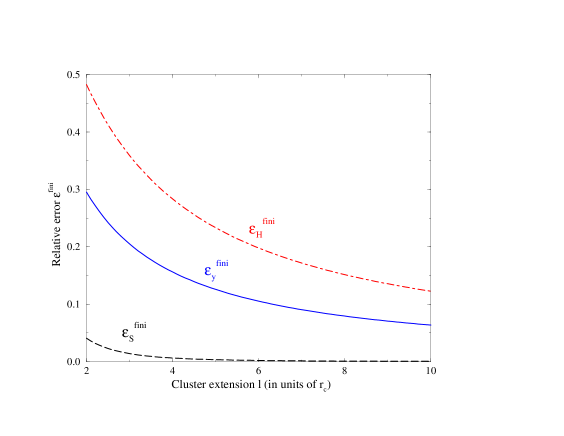
Figure 2: Influence of the finite extension on the Compton parameter, the surface brightness and the Hubble constant assuming $\beta=2/3$, $r_{x}=r_{z}=0$ and a spherical cluster. The relative errors which are shown are defined in the text.

We denote $y(\infty)$ and $S_{X}(\infty)$, respectively, as the expressions of the Compton parameter and of the X-ray surface brightness for a cluster with infinite extension, and $y(l)$ and $S_{X}(l)$ as the same expressions for a cluster with a finite extension $l$ along the line of sight. The relative errors $\epsilon_{y}^{fini}$ on the Compton parameter and $\epsilon_{S}^{fini}$ on the surface brightness are defined by the expressions:

$$\epsilon_{y}^{fini}=\frac{y(\infty)-y(l)}{y(\infty)}\ \ {\rm and}\ \ \epsilon_{S}^{fini}=\frac{S_{X}(\infty)-S_{X}(l)}{S_{X}(\infty)}\leavevmode\nobreak\ .$$ (13)

¿From Eqs. (9) and (10) we can easily estimate these ratios which are

$$\epsilon_{y}^{fini}=\frac{B_{m}(3/2\beta-1/2,1/2)}{B(3/2\beta-1/2,1/2)}\ \ {\rm and}\ \ \epsilon_{S}^{fini}=\frac{B_{m}(3\beta-1/2,1/2)}{B(3\beta-1/2,1/2)}\leavevmode\nobreak\ .$$ (14)

For a spherical density profile, a line of sight through the cluster center and an infinite extension, we obtain from Eq. (12):

$$\frac{y^{2}(\infty)}{S_{X}(\infty)}=\lambda T_{eo}^{3/2}\,r_{c}\,\frac{\left[B(\frac{3}{2}\beta-\frac{1}{2},\frac{1}{2})\right]^{2}}{B(3\beta-\frac{1}{2},\frac{1}{2})}\leavevmode\nobreak\ .$$ (15)

We introduce $\theta_{c}=r_{c}/D_{A}$ the angular core radius, where $D_{A}$ is the angular diameter distance of the cluster:

$$D_{A}=\frac{{\cal C}}{H_{0}}\ \ {\rm where}\ \ {\cal C}=\frac{c}{q_{0}^{2}}\frac{q_{0}z+(q_{0}-1)(\sqrt{1+2q_{0}z}-1)}{(1+z)^{2}}.$$ (16)

With Eq. (15) we can estimate the Hubble constant $H_{0}(\infty)$ for an infinitely extended cluster by:

$$H_{0}(\infty)=\lambda^{\prime}\,T_{eo}^{3/2}\,\frac{S_{X}(\infty)}{y^{2}(\infty)}\,\theta_{c}\,\frac{\left[B(\frac{3}{2}\beta-\frac{1}{2},\frac{1}{2})\right]^{2}}{B(3\beta-\frac{1}{2},\frac{1}{2})}\ \ {\rm with}\ \ \lambda^{\prime}=\lambda{\cal C}$$ (17)

and for a finite extension $l$, we get instead

$$H_{0}(l)=\lambda^{\prime}T_{eo}^{3/2}\,\frac{S_{X}(l)}{y^{2}(l)}\,\theta_{c}\,\frac{\left[B\left(\frac{3}{2}\beta-\frac{1}{2},\frac{1}{2}\right)-B_{m}\left(\frac{3}{2}\beta-\frac{1}{2},\frac{1}{2}\right)\right]^{2}}{\left[B\left(3\beta-\frac{1}{2},\frac{1}{2}\right)-B_{m}\left(3\beta-\frac{1}{2},\frac{1}{2}\right)\right]}.$$ (18)

Obviously, $S_{X}$ and $y^{2}$ are observed quantities and thus the ratios $S_{X}(\infty)/y^{2}(\infty)$ and $S_{X}(l)/y^{2}(l)$ are in the following both set equal to the measured value $\Bigl{(}S_{X}/y^{2}\Bigr{)}_{obs}$. This way, for our example, we get for the relative error for the estimation of the Hubble constant, due to assuming an infinite extension rather than a finite one, the expression:

$$\epsilon_{H_{0}}^{fini}=\frac{H_{0}(\infty)-H_{0}(l)}{H_{0}(\infty)}=1-\frac{B(3\beta-\frac{1}{2},\frac{1}{2})\left[B(\frac{3}{2}\beta-\frac{1}{2},\frac{1}{2})-B_{m}(\frac{3}{2}\beta-\frac{1}{2},\frac{1}{2})\right]^{2}}{B^{2}(\frac{3}{2}\beta-\frac{1}{2},\frac{1}{2})\left[B(3\beta-\frac{1}{2},\frac{1}{2})-B_{m}(3\beta-\frac{1}{2},\frac{1}{2})\right]}\leavevmode\nobreak\ .$$ (19)

In Fig. (2) we plot the relative error as a function of the finite extension $l$ for a spherical isothermal $\beta=2/3$-model. For $l\rightarrow\infty$ the relative errors on the Compton parameter, the X-ray surface brightness and the Hubble parameter become, of course, negligible. For instance, for a cluster with a finite extension of about 10 times $r_{c}$, the relative error with respect to the assumption of an infinite extension is only about 6 % for the Compton parameter. For the X-ray surface brightness, the relative error due to the finite extension is much smaller, for instance an error of about 4% is obtained if the cluster has an extension of only about 2 times $r_{c}$. Nevertheless, for clusters with a small extension (3$r_{c}$) with respect to their core radius, the error in $\epsilon_{y}^{fini}$ becomes quite substantial ($\sim 20$%) for the Compton parameter.
These estimations are in accordance with the results of Inagaki et al. (Ina95 (1995)). The net effect when one considers infinite clusters is thus to overestimate the value of the temperature decrement and the X-ray surface brightness.
The influence of the finite extension on the Hubble constant given in Eq. (19) is larger. Indeed, the Hubble parameter is overestimated by almost 20%, when considering for instance a cluster with infinite extension as compared to one with an extension of 7$r_{c}$ (cf. Fig. 2).

3.2 Polytropic index

Although the isothermal distribution is often a reasonable approximation of the actual observed clusters, some clusters do show non-isothermal features. Henriksen & Mushotzky (hen85 (1985)) have suggested that the isothermal model cannot be consistently applied to gas distributions in clusters. Indeed, Markevitch et al. (Mar98 (1998)) find that the temperature profiles of some clusters can be approximately described by a polytrope. More recently, Ettori et al. (Ett00 (2000)), with a combined analysis of the BeppoSAX and ROSAT-PSPC observations, showed that a polytropic profile with index $\gamma=1.16\pm 0.03$ fits the temperature distribution of the cluster A3562 very closely.
As a consequence, within the virial regions of typical clusters of galaxies, the gravitating mass, the gas mass and the gas fraction can vary quite substantially, compared to that obtained assuming an isothermal profile (Ettori & Fabian Ett99 (1999), Ettori Ett00 (2000), Ettori et al. Eta00 (2000)). It is interesting, therefore, to investigate the variations due to a polytropic equation of state on SZ quantities.
A polytropic thermal profile has the following form:

$$T_{e}=T_{eo}\,\left[\frac{n_{e}}{n_{eo}}\right]^{\gamma-1}\leavevmode\nobreak\ ,$$ (20)

where the subscript $o$ denotes the values in the cluster center and $\gamma$ is the polytropic index. The isothermal profile is obtained by setting $\gamma=1$.
Then the Compton parameter and surface brightness are given by

$$y^{poly}=2\,\frac{k_{B}T_{eo}n_{eo}r_{c}\sigma_{T}}{m_{e}c^{2}}\,\int_{0}^{l}\,\left[\frac{n_{e}}{n_{eo}}\right]^{\gamma}dr_{y}$$ (21)

$$S_{X}^{poly}=\frac{\epsilon\sqrt{T_{eo}}n_{eo}^{2}r_{c}}{2\pi(1+z)^{3}}\,\int_{0}^{l}\,\left(\frac{n_{e}}{n_{eo}}\right)^{\frac{\gamma}{2}+\frac{3}{2}}\,dr_{y}.$$ (22)

Similarly to the calculations in Section 2, we find for $y^{poly}$ and $S_{X}^{poly}$:

$$y^{poly}(r_{x},r_{z})= \frac{k_{B}T_{eo}\zeta_{2}r_{c}\sigma_{T}n_{eo}}{m_{e}c^{2}}\,\times\,\left(1+\frac{r_{x}^{2}}{\zeta_{1}^{2}}+\frac{r_{z}^{2}}{\zeta_{3}^{2}}\right)^{-\frac{3}{2}\beta\gamma+\frac{1}{2}}$$ (23)

$$\times \,\left[B\left(\frac{3}{2}\beta\gamma-\frac{1}{2},\frac{1}{2}\right)-B_{m}\left(\frac{3}{2}\beta\gamma-\frac{1}{2},\frac{1}{2}\right)\right]\leavevmode\nobreak\ ,$$

$$S_{X}^{poly}(r_{x},r_{z})= \frac{\epsilon\sqrt{T_{eo}}n_{eo}^{2}\zeta_{2}r_{c}}{4\pi(1+z)^{3}}\,\times\,\left(1+\frac{r_{x}^{2}}{\zeta_{1}^{2}}+\frac{r_{z}^{2}}{\zeta_{3}^{2}}\right)^{-\frac{3}{2}\beta(\frac{\gamma}{2}+\frac{3}{2})+\frac{1}{2}}$$ (24)

$$\times \,\left[B\left(\frac{3}{2}\beta\left(\frac{\gamma}{2}+\frac{3}{2}\right)-\frac{1}{2},\frac{1}{2}\right)-B_{m}\left(\frac{3}{2}\beta\left(\frac{\gamma}{2}+\frac{3}{2}\right)-\frac{1}{2},\frac{1}{2}\right)\right]\leavevmode\nobreak\ .$$

The relative error by considering a polytropic profile (index $poly$) as compared to an isothermal profile (index $iso$), can be expressed as follows, assuming for simplicity an infinite extension of the cluster,

$$\epsilon_{y}^{poly} = \frac{y_{iso}-y_{poly}}{y_{iso}}$$

$$= 1-\left[1+\left(\frac{r_{x}}{\zeta_{1}}\right)^{2}+\left(\frac{r_{z}}{\zeta_{3}}\right)^{2}\right]^{-\frac{3}{2}\beta(\gamma-1)}\times\frac{B\left(\frac{3}{2}\beta\gamma-\frac{1}{2},\frac{1}{2}\right)}{B\left(\frac{3}{2}\beta-\frac{1}{2},\frac{1}{2}\right)}$$

for the Compton parameter and

$$\epsilon_{S}^{poly} = \frac{\left(S_{X}\right)_{iso}-\left(S_{X}\right)_{poly}}{\left(S_{X}\right)_{iso}}$$

$$= 1-\left[1+\left(\frac{r_{x}}{\zeta_{1}}\right)^{2}+\left(\frac{r_{z}}{\zeta_{3}}\right)^{2}\right]^{-\frac{3}{4}\beta(\gamma-1)}\times\frac{B\left(\frac{3}{2}\beta(\frac{\gamma}{2}+\frac{3}{2})-\frac{1}{2},\frac{1}{2}\right)}{B\left(3\beta-\frac{1}{2},\frac{1}{2}\right)}$$

for the surface brightness.
The corresponding error for the Hubble constant turns out to be

$$\epsilon_{H}^{poly}=\frac{\left(H_{0}\right)_{iso}-\left(H_{0}\right)_{poly}}{\left(H_{0}\right)_{iso}}=1-\frac{\left[B\left(\frac{3}{2}\beta\gamma-\frac{1}{2},\frac{1}{2}\right)\right]^{2}B(3\beta-\frac{1}{2},\frac{1}{2})}{\left[B\left(\frac{3}{2}\beta-\frac{1}{2},\frac{1}{2}\right)\right]^{2}B(\frac{3}{2}\beta(\frac{\gamma}{2}+\frac{3}{2})-\frac{1}{2},\frac{1}{2})}\leavevmode\nobreak\ ,$$ (27)

when taking measurements along the line of sight going through the cluster center. The relative errors defined above for polytropic indices between 1 and 2 are shown in Fig. (3).

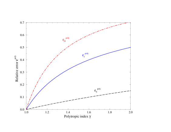
Figure 3: Relative error $\epsilon_{y}^{poly}$ (for $\Delta T_{SZ}$), $\epsilon_{S}^{poly}$ (for $S_{X}$) and $\epsilon_{H}^{poly}$ for the Hubble constant between a polytropic and an isothermal profile. The line of sight is taken to go through the center of the cluster, which is assumed to have a spherical profile with infinite extension ($\beta=2/3$-model).

Already, a small deviation from the isothermal case ($\gamma=1$) leads to significant relative errors and thus to quite different values of the observable quantities. For instance, assuming an isothermal instead of a polytropic profile with index $\gamma=1.2$ leads to an overestimation of 20%, 4% and 34% for the quantities $y,\leavevmode\nobreak\ S_{X}$ and $H_{0}$, respectively.

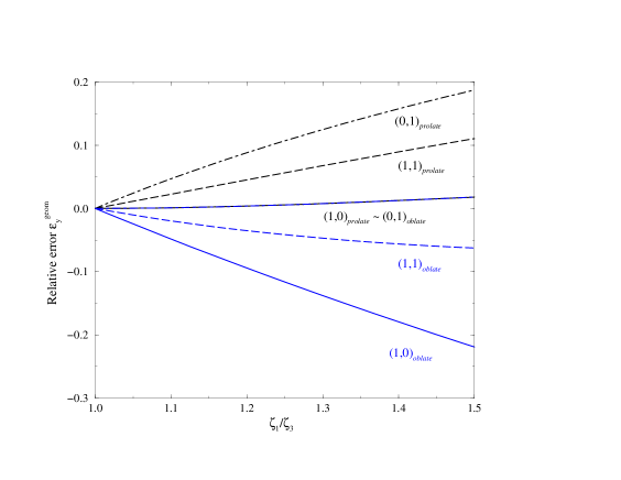
Figure 4: Geometrical relative error $\epsilon_{y}^{geom}$ for $y$ between an axisymmetric ellipsoidal and a spherical geometry (assuming infinite extension, isothermal profile and $\beta=2/3$) for three different lines of sight, parametrized in units of $r_{c}$. The two ellipsoidal shapes $prolate$ and $oblate$ are indicated.

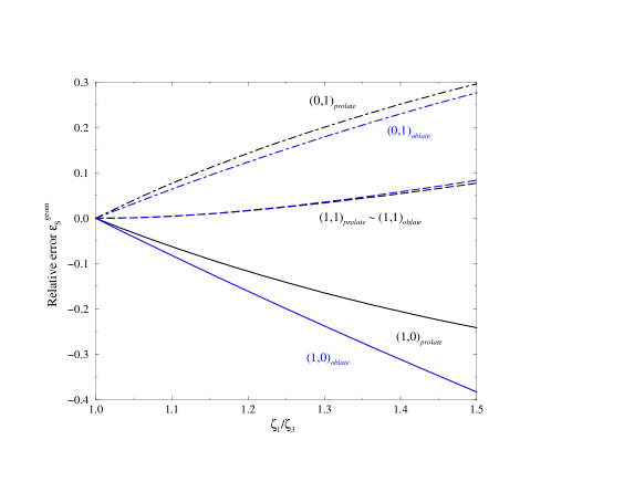
Figure 5: Geometrical relative error $\epsilon_{S}^{geom}$ for $S_{X}$ between an axisymmetric ellipsoidal and a spherical geometry (assuming infinite extension, isothermal profile and $\beta=2/3$) for three different lines of sight, parametrized in units of $r_{c}$. The two ellipsoidal shapes $prolate$ and $oblate$ are indicated.

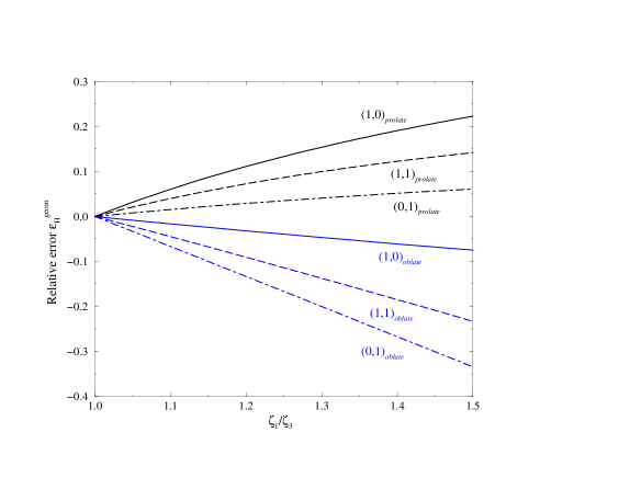
Figure 6: Geometrical relative error $\epsilon_{H}^{geom}$ for $H$ between an axisymmetric ellipsoidal and a spherical geometry (assuming infinite extension, isothermal profile and $\beta=2/3$) for three different lines of sight, parametrized in units of $r_{c}$. The two ellipsoidal shapes $prolate$ and $oblate$ are indicated.

3.3 Geometrical effect

In order to compare the relative errors induced by geometrical effects, i.e. the difference between ellipsoidal and spherical geometries, we choose the parameters of the cluster for both geometries such that we get the same value for the emission integral EI, defined by Sarazin (Sar88 (1988)) as:

$${\rm EI}=\int\,n_{e}^{2}\,dV,$$ (28)

where $V$ is the volume of the cluster. We consider, for simplicity, the case where the various integrals are approximated by assuming an infinite extension: after some algebra (see Appendix A for the change of variables) we get the following expression for the emission integral for a spherical geometry:

$$EI_{sph}=\pi^{3/2}n_{eo}^{2}r_{c}^{3}\,\frac{\Gamma(3\beta-\frac{3}{2})}{\Gamma(3\beta)}\leavevmode\nobreak\ ,$$ (29)

and for an ellipsoidal geometry:

$$EI_{ell}=\pi^{3/2}n_{eo}^{2}\zeta_{1}\zeta_{2}\zeta_{3}r_{c}^{3}\,\frac{\Gamma(3\beta-\frac{3}{2})}{\Gamma(3\beta)}\leavevmode\nobreak\ .$$ (30)

Thus the equal emission condition $EI_{sph}=EI_{ell}$ requires $\zeta_{1}\;\zeta_{2}\;\zeta_{3}=1$.
In the following we will consider the two axisymmetric cases prolate (cigar shaped) with symmetry axis $r_{x}$, thus $\zeta_{2}=\zeta_{3}=\sqrt{1/\zeta_{1}}$, and oblate (pancake shaped), where the symmetry axis is given by $r_{z}$, and thus $\zeta_{2}=\zeta_{1}$ and $\zeta_{3}=1/\zeta_{1}^{2}$.

We introduce $\epsilon_{y}^{geom}$ and $\epsilon_{S}^{geom}$ as the geometrical relative error between ellipsoidal and spherical geometry for the Compton parameter and the surface brightness, respectively,

$$\epsilon_{y}^{geom}=\frac{y_{sph}-y_{ell}}{y_{sph}}\ \ {\rm and}\ \ \epsilon_{S}^{geom}=\frac{\left(S_{X}\right)_{sph}-\left(S_{X}\right)_{ell}}{\left(S_{X}\right)_{sph}}\leavevmode\nobreak\ ,$$ (31)

and thus find

$$\epsilon_{y}^{geom}\,=\,1-\zeta_{2}\leavevmode\nobreak\ \left(\frac{1+\frac{r_{x}^{2}}{\zeta_{1}^{2}}+\frac{r_{z}^{2}}{\zeta_{3}^{2}}}{1+r_{x}^{2}+r_{z}^{2}}\right)^{-\frac{3}{2}\beta+\frac{1}{2}}\,\,\leavevmode\nobreak\ {\rm and}$$ (32)

$$\epsilon_{S}^{geom}=1-\zeta_{2}\leavevmode\nobreak\ \left(\frac{1+\frac{r_{x}^{2}}{\zeta_{1}^{2}}+\frac{r_{z}^{2}}{\zeta_{3}^{2}}}{1+r_{x}^{2}+r_{z}^{2}}\right)^{-3\beta+\frac{1}{2}}\leavevmode\nobreak\ .$$ (33)

In Figs. (4) and (5) we have plotted the geometrical relative error as a function of the flattening of the profile $\zeta_{1}/\zeta_{3}$ for the Compton parameter $\epsilon_{y}^{geom}$ and the surface brightness $\epsilon_{S}^{geom}$, respectively. We consider three different lines of sight, $(r_{x},r_{z})$ = (1,0), (1,1) and (0,1), given in units of the core radius $r_{c}$.
Fig. (4) shows, that the line of sight (1,0) in the prolate case leads to almost the same error of the Compton parameter as the line of sight (0,1) in the oblate case. For a flattening of 50% (i.e. $\zeta_{1}/\zeta_{3}\leavevmode\nobreak\ =\leavevmode\nobreak\ 1.5$) we get an overestimation of about 2% by using a spherical cluster shape instead of an ellipsoidal one. The other lines of sight lead in the prolate case to overestimations of up to 19%, while in the oblate case the Compton parameter is underestimated by almost 22%.
Due to a quadratic dependance on the density profile, the surface brightness is more affected by a flattened shape. The line of sight (1,1) shows in both cases (prolate and oblate) an overestimation of about 8%. Towards (0,1) the surface brightness is overestimated in both cases by up to 30%, while the view towards (1,0) results in an underestimation of 24% for a prolate deformation and almost 38% in the oblate case.

In the case of an infinite extension approximation from Eq. (12) we get

$$\frac{y^{2}(r_{x},r_{z})}{S_{X}(r_{x},r_{z})}=\lambda\,T_{eo}^{3/2}\,\zeta_{2}r_{c}\,\times\left(1+\frac{r_{x}^{2}}{\zeta_{1}^{2}}+\frac{r_{z}^{2}}{\zeta_{3}^{2}}\right)^{\frac{1}{2}}\times\frac{B^{2}\left(\frac{3}{2}\beta-\frac{1}{2},\frac{1}{2}\right)}{B\left(3\beta-\frac{1}{2},\frac{1}{2}\right)}\leavevmode\nobreak\ .$$ (34)

Again, the ratio $y^{2}/S_{X}$ ratio is set equal to the observed value and leads then to the relative error on the Hubble constant:

$$\epsilon_{H}^{geom}=\frac{\left(H_{0}\right)_{sph}-\left(H_{0}\right)_{ell}}{\left(H_{0}\right)_{sph}}=1-\zeta_{2}\leavevmode\nobreak\ \left(\frac{1+\frac{r_{x}^{2}}{\zeta_{1}^{2}}+\frac{r_{z}^{2}}{\zeta_{3}^{2}}}{1+r_{x}^{2}+r_{z}^{2}}\right)^{\frac{1}{2}}\leavevmode\nobreak\ .$$ (35)

Fig. (6) shows in the axisymmetric ellipsoidal cases, prolate and oblate, the influence of a flattening of the cluster profile up to 50%. The prolate case results in a systematic overestimation of the Hubble constant, by considering a spherical instead of a flattened profile. Depending on the line of sight, this error goes up to 22%. Underestimations of up to 33% arise in the oblate case.
We summarize in Table (1) the relative errors on the $y$-parameter, the surface brightness and the Hubble constant that appear by considering a spherical instead of a flattened ellipsoidal shape with, as an example, an axis ratio of 1.2. Negative values indicate that the considered quantity is underestimated, whereas positive values that it is overestimated.

Cluster shape	Line of sight	$\epsilon_{y}^{geom}$	$\epsilon_{S}^{geom}$	$\epsilon_{H}^{geom}$
	(in $r_{c}$)	(in %)	(in %)	(in % )
prolate	(1,0)	0.4	-11.7	11.1
	(1,1)	4.5	1.7	7.3
	(0,1)	8.8	14.3	2.9
oblate	(1,0)	-9.4	-16.1	-3.2
	(1,1)	-3.5	1.7	-9.1
	(0,1)	0.4	12.4	-13.3

Table 1: Relative errors on the $y$-parameter, the surface brightness and the Hubble constant are shown. The flattened ellipsoidal is supposed to have an axes ratio of 1.2. Negative numbers indicate underestimations, whereas positive ones overestimations.

In the general triaxial case (i.e. not necessarily prolate or oblate), estimating the Hubble constant is more difficult. We can compute the angular diameter distance $D_{A}$ and thus the Hubble constant by measuring the angles $\theta_{1}$ and $\theta_{3}$, defined as the angular ellipsoidal core radii $\theta_{1}=\zeta_{1}r_{c}/D_{A}$ and $\theta_{3}=\zeta_{3}r_{c}/D_{A}$, but we have no observational access to the corresponding angle $\theta_{2}$. On the contrary, in the case of a spherical profile it is sufficient to measure, as we have seen in section (3.1), the value of $y$ and $S_{X}$ towards the center of the cluster in order to evaluate the Hubble constant. We do not discuss further the geometrical relative error for a general triaxial cluster.

3.4 Projection effect

Ruiz (Rui76 (1976)) and Stark (Sta77 (1977)) have discussed the projection onto the sky of luminosity distributions which have an ellipsoidal form. This problem has also been treated by Fabricant, Rybicki & Gorenstein (Fab84 (1984)). The projection effect is expected to broaden the measurements of the temperature decrement and the surface brightness as mentioned by Cooray (Coo98 (1998)).
In order to evaluate the projection effect we assume an ellipsoidal geometry. As an example, we take the case of an infinite cluster extension with isothermal profile and a prolate form.
The profile of the cluster is supposed to be rotated by an angle $\theta$ around the $r_{z}$ axis. For comparison, we consider a prolate profile with a major half axis along $r_{x}$, which has the same projected image on the sky, i.e. on the ($r_{x},r_{z}$)-plane. We then compute the difference on the resulting $y$-parameter and surface brightness between these two profiles. The structure integrals $I^{proj}$ and $I^{rot}$ are given in Appendix B, where we have computed the $y$ parameter and the surface brightness of a cluster both for a rotated coordinate system, with an angle $\theta$, and by considering its projection onto the sky.
The relative error can be quantified as

$$\epsilon_{I}^{proj}=\frac{I^{proj}-I^{rot}}{I^{proj}}\leavevmode\nobreak\ .$$ (36)

It is a pure geometrical effect and thus the same for the $y$ parameter, the surface brightness and the Hubble constant.

In Figs. (7) and (8) we have plotted the relative error due to the projection effects as a function of the rotation angle $\theta$ and the axes ratio $\zeta_{1}/\zeta_{3}$ of the ellipsoid.

Figure 7: The relative error, when comparing a projected and a rotated prolate-shaped cluster, is shown as a function of $\theta$. The axis ratio is fixed to be $\zeta_{1}/\zeta_{3}=1.5$.

Figure 8: The relative error between a projected and a rotated prolate-shaped cluster profile is shown as a function of the axes ratio $\zeta_{1}/\zeta_{3}$. The rotation angle $\theta$ is fixed at $\pi/4$.

The maximal $\theta$ is assumed to be $\pi/4\sim 0.785$, for which we find an underestimation of almost 17%. The influence of the axes ratio turns out to be less than 5%.

4 Discussion and conclusions

We have calculated the relative error caused by assumptions regarding finite extension, a polytropic temperature profile, ellipsoidal geometry and projection effects, on the measurements of the X-ray surface brightness, the SZ temperature decrement and the determination of the Hubble constant. Although the X-ray data have improved dramatically in the last decade, it is still difficult to determine the internal structure of clusters from X-ray imaging alone, because such images supply only projected temperature and surface brightness information, without further indications of the internal gas dynamics. Nevertheless, recent observations show indirectly that many clusters are still dynamically evolving (see Mohr et al. mo95 (1995)).
Cooray (Coo2000 (2000)) has discussed intrinsic cluster shape, in particular considering axisymmetric models such as oblate and prolate ellipsoids, using the Mohr et al. (mo95 (1995)) cluster sample. Their study shows that clusters do indeed have aspherical profiles, which are more likely described as prolate rather than oblate ellipsoids. Nevertheless, Mohr et al. (mo95 (1995)) remarked that they cannot rule out the possibility that clusters are intrinsically triaxial.

Pierre et al. (Pie96 (1996)) studied with ROSAT the rich lensing cluster Abell 2390 and determined its gas and matter content. They found that on large scales the $X$-ray distribution has an elliptical shape with an axis ratio of minor to major half axis of $\zeta_{1}/\zeta_{3}\sim 1.33$. Using our results we see that this corresponds to a relative error in the $y$ parameter of up to 10%, depending on the line of sight and the shape of the cluster (prolate or oblate, see Fig. 4). The surface brightness measurements lead to errors of up to 25% (see Fig. 5) and thus the Hubble constant is overestimated by about 23% (see Fig. 6).

An unresolved temperature gradient in the gas affects the gas profile and thus the total mass derived assuming hydrostatic equilibrium. If such a gradient is present, the true temperature in the central region may be higher than the emission-weighted temperature generally used. As an example, Grego et al. (gre2000 (2000)) observed in Abell 370 a slow decline of the temperature with radius. The temperature falls to half its central value within 6-10 core radii. This temperature profile can be approximately described by a gas with a polytropic index of $\gamma=1.2$, which in itself is already an important modification with respect to an isothermal profile and could lead to a relative error $\epsilon^{poly}_{H}$ of 37% in the evaluation of the Hubble constant (see Fig. 3).
Furthermore, the optical and X-ray observations of this cluster show a possible bimodal mass distribution. Thus, the combined temperature and geometry effects must be taken into account to obtain reliable values for such parameters as the gas and total matter content. A similar polytropic index ($\gamma=1.16$) has also been found for Abell 3562 (Ettori et al. Ett00 (2000)).

Cooling flows in galaxy clusters can substantially change the temperature profiles, especially in the inner regions. Schlickeiser (Sch91 (1991)) and Majumdar & Nath (maju2000 (2000)) have investigated the changes induced by a cooling flow in the temperature and density profiles, and their implications on the SZ effect. We notice that for a polytropic distribution, the density profile can still be well approximated by a $\beta$ profile, whereas for cooling flow solutions the density becomes quite different. For example, Vikhlinin et al. (vik99 (1999)) showed that outside the cooling flow region, the $\beta$-model describes the observed surface brightness closely, but not precisely. In this context, Majumdar & Nath (maju2000 (2000)) found that the presence of a cooling flow in a cluster can lead to an overestimation of the Hubble constant determined from the SZ decrement. Recently, Mauskopf, Ade, Allen et al. (maus2000 (2000)) determined the Hubble constant from $X$-ray measurements obtained of the cluster Abell 1835 with ROSAT and from the corresponding millimetric observations of the SZ effect with the Sunyaev-Zel’dovich Infrared Experiment (Suzie) multifrequency array receiver. Assuming an infinitely extended, spherical gas distribution with an isothermal equation of state, characterized by $\beta=0.58\pm 0.02$, $T_{eo}=9.8^{+2.3}_{-1.3}$ keV and $n_{eo}=5.64^{+1.61}_{-1.02}\times 10^{-2}$ cm^-3, they found a value of $H_{o}=59^{+38}_{-28}$ km s^-1 Mpc^-1 for the Hubble constant. In Fig. (9) we show the influence of geometry and of assumptions of finite extension on this result using the same input parameters. Fig. (9a) shows that for a spherical geometry, $H_{o}$ displays a strong dependence on the cluster extension. Fig. (9b) gives the value of $H_{o}$ assuming an infinite extended ellipsoid shaped cluster (instead of a spherical geometry), as a function of its axis ratio $\zeta_{1}/\zeta_{3}$.

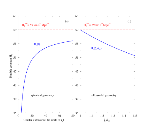
Figure 9: The Hubble constant derived from the data of Mauskopf et al. (2000). Fig. (9a) shows the influence of finite extension, while Fig. (9b) gives the value of $H_{o}$ assuming an axisymmetric ellipsoidal geometry. In the latter case, oblate or prolate geometry give the same value of $H_{o}$ when taking a line of sight through the cluster center, as is assumed here.

In summary, we see that it is crucial to know the shape of a cluster and its temperature profile. For this problem, the new X-ray satellites have the necessary spatial and spectral resolution to remove the effects of contaminating sources in the field and to measure the spatial variation of the cluster temperature. In this context it will be better for future studies to focus on nearby cluster samples, which are less subject to observational selection effects (as mentioned by Roettiger et al., (Roe97 (1997))).

Appendix A

Structure integral for the $\@vec{y}$ parameter
The structure integral for the SZ effect is given by the expression

$$I_{SZ}(r_{x},r_{z})=\,2\,\int_{0}^{l}\,\frac{n_{e}}{n_{eo}}dr_{y},$$ (37)

where $n_{e}$ is the density profile of the electrons, $n_{eo}$ the central density of the cluster and $l$ the maximum extension of the hot gas on the line of sight $r_{y}$, in units of the core radius $r_{c}$. With an ellipsoidal density profile, we obtain

$$I_{SZ}(r_{x},r_{z})\,=\,2\,\int_{0}^{l}\,\left[1+\frac{r_{x}^{2}}{\zeta_{1}^{2}}+\frac{r_{y}^{2}}{\zeta_{2}^{2}}+\frac{r_{z}^{2}}{\zeta_{3}^{2}}\right]^{-\frac{3}{2}\beta}\,dr_{y}\leavevmode\nobreak\ ,$$ (38)

where $r_{i},\leavevmode\nobreak\ \zeta_{i}$ and $l$ are given in units of the core radius $r_{c}$. With the definition of a function $G$ and transforming the variable of integration from $r_{y}$ to $\xi$ such that

$$G(\xi)=\left(1+\xi\right)^{-3\beta/2}\ {\rm with}\ \ \xi=\frac{r_{x}^{2}}{\zeta_{1}^{2}}+\frac{r_{y}^{2}}{\zeta_{2}^{2}}+\frac{r_{z}^{2}}{\zeta_{3}^{2}}\leavevmode\nobreak\ ,$$

we obtain after some algebra the structure integral

$$I_{SZ}(r_{x},r_{z})=\int_{\eta}^{\eta+(l/\zeta_{2})^{2}}G(\xi)\,(\xi-\eta)^{-1/2}\,d\xi\leavevmode\nobreak\ ,\ \ {\rm where}\ \ \eta=\frac{r_{x}^{2}}{\zeta_{1}^{2}}+\frac{r_{z}^{2}}{\zeta_{3}^{2}}\leavevmode\nobreak\ .$$ (39)

Finally, with a last change of variable,

$$\alpha=\frac{1+\eta}{1+\xi}\leavevmode\nobreak\ ,$$

we get

$$I_{SZ}(r_{x},r_{z})=\zeta_{2}\leavevmode\nobreak\ (1+\eta)^{-3(\beta+1)/2}\,\int_{m}^{1}\,\alpha^{(3\beta-3)/2}\,\,(1-\alpha)^{-1/2}\,d\alpha$$ (40)

with

$$m=\frac{1+\eta}{1+\eta+(l/\zeta_{2})^{2}}\leavevmode\nobreak\ .$$

The structure integral turns out to be

$$I_{SZ}(r_{x},r_{z})=\zeta_{2}\leavevmode\nobreak\ (1+\eta)^{-\frac{3}{2}\beta+\frac{1}{2}}\leavevmode\nobreak\ \left[B\left(\frac{3}{2}\beta-\frac{1}{2},\frac{1}{2}\right)-B_{m}\left(\frac{3}{2}\beta-\frac{1}{2},\frac{1}{2}\right)\right]\leavevmode\nobreak\ ,$$ (41)

where we introduced the Beta and the incomplete Beta functions defined by

$$B(a,b)=\frac{\Gamma(a)\Gamma(b)}{\Gamma(a+b)}$$

and

$$B_{m}(a,b)=\frac{\Gamma_{m}(a)\Gamma_{m}(b)}{\Gamma_{m}(a+b)}\leavevmode\nobreak\ ,$$

with the Gamma and the incomplete Gamma-functions $\Gamma$ and $\Gamma_{m}$, respectively.

$\@vec{X}$-ray surface brightness
The structure integral for the $X$-ray surface brightness is given by

$$I_{S_{X}}=2\,\int_{0}^{l}\,\left[\frac{n_{e}}{n_{eo}}\right]^{2}dr_{y}.$$ (42)

With the same transformations, as given above, we get

$$I_{S_{X}}(r_{x},r_{z})=\zeta_{2}\leavevmode\nobreak\ (1+\eta)^{-3\beta+\frac{1}{2}}\,\left[B\left(3\beta-\frac{1}{2},\frac{1}{2}\right)-B_{m}\left(3\beta-\frac{1}{2},\frac{1}{2}\right)\right]\leavevmode\nobreak\ .$$ (43)

Appendix B

Projection effects on the $\@vec{y}$ parameter The rotation in the ($r_{x},r_{y}$)-plane around $r_{z}$ with an angle $\theta$ leads to the density profile:

$$n_{e}^{rot}(r_{x},r_{y},r_{z},\theta)=n_{eo}\left[1+\frac{(r_{x}\,{\rm cos}\theta+r_{y}\,{\rm sin}\theta)^{2}}{\zeta_{1}^{2}}+\frac{(r_{y}\,{\rm cos}\theta-r_{x}\,{\rm sin}\theta)^{2}}{\zeta_{2}^{2}}+\frac{r_{z}^{2}}{\zeta_{3}^{2}}\right]^{-3\beta/2}.$$ (44)

The rotation angle $\theta$ is the angle between the major half axis of the rotated ellipse in the $(r_{x},r_{y})$ plane and the $r_{x}$-axis. The line of sight is taken to be along the $r_{y}$-axis.
To investigate the projection effects we will compare a rotated cluster with respect to the $r_{z}$ axis with its projection on the ($r_{x},r_{z}$) plane, corresponding to the sky plane. We assume an infinite extension and an isothermal profile.
The rotated structure integral for the $y$ parameter turns out to be

$$I_{SZ}^{rot}(r_{x},r_{z},\theta)=\int_{-\infty}^{\infty}\,\left[1+\frac{(r_{x}\,{\rm cos}\theta+r_{y}\,{\rm sin}\theta)^{2}}{\zeta_{1}^{2}}+\frac{(r_{y}\,{\rm cos}\theta-r_{x}\,{\rm sin}\theta)^{2}}{\zeta_{2}^{2}}+\frac{r_{z}^{2}}{\zeta_{3}^{2}}\right]^{-3\beta/2}\,dr_{y}\leavevmode\nobreak\ .$$ (45)

After some algebra and with the same kind of variable changes as in Appendix A, we get (assuming an infinite cluster extension for the structure integral):

$$I_{SZ}^{rot}(r_{x},r_{z},\theta)=\frac{1}{\sqrt{\frac{{\rm cos}^{2}\theta}{\zeta_{2}^{2}}+\frac{{\rm sin}^{2}\theta}{\zeta_{1}^{2}}}}\leavevmode\nobreak\ (1+\eta_{\theta})^{-\frac{3}{2}\beta+\frac{1}{2}}\leavevmode\nobreak\ B\left(\frac{3}{2}\beta-\frac{1}{2},\frac{1}{2}\right)\leavevmode\nobreak\ ,$$ (46)

with

$$\eta_{\theta}=\frac{r_{x}^{2}}{\zeta_{1}^{2}{\rm cos}^{2}\theta+\zeta_{2}^{2}{\rm sin}^{2}\theta}+\frac{r_{z}^{2}}{\zeta_{3}^{2}}\leavevmode\nobreak\ .$$

On the other hand, the projection of this cluster on the observed sky plane in the infinite cluster extension case leads to the density profile

$$n_{e}^{proj}(r_{x},r_{y},r_{z})=n_{eo}\left[1+\frac{r_{x}^{2}}{\tilde{\zeta}_{1}^{2}}+\frac{r_{y}^{2}}{\tilde{\zeta}_{2}^{2}}+\frac{r_{z}^{2}}{\tilde{\zeta}_{3}^{2}}\right]^{-3\beta/2}\leavevmode\nobreak\ ,$$ (47)

where $\tilde{\zeta_{1}}$ is the maximum value that we get along the $r_{x}$ axis in units of $r_{c}$

$$\tilde{\zeta}_{1}=\sqrt{\zeta_{1}^{2}\cos^{2}\theta+\zeta_{2}^{2}\sin^{2}\theta}\leavevmode\nobreak\ ,$$

moreover, $\tilde{\zeta_{3}}/\tilde{\zeta_{2}}=\zeta_{3}/\zeta_{2}=1$ (prolate).
The projected structure integral for the $y$ parameter turns out to be

$$I_{SZ}^{proj}(r_{x},r_{z},\theta)=\tilde{\zeta_{2}}\leavevmode\nobreak\ (1+\tilde{\eta_{\theta}})^{-\frac{3}{2}\beta+\frac{1}{2}}\leavevmode\nobreak\ B\left(\frac{3}{2}\beta-\frac{1}{2},\frac{1}{2}\right)$$ (48)

with

$$\tilde{\eta_{\theta}}=\frac{r_{x}^{2}}{\tilde{\zeta_{1}}^{2}}+\frac{r_{z}^{2}}{\tilde{\zeta_{3}}^{2}}\leavevmode\nobreak\ .$$

$\@vec{X}$-ray surface brightness For the structure integral of the $X$-ray surface brightness we find in the case of the rotated cluster

$$I_{S_{X}}^{rot}(r_{x},r_{z},\theta)=\frac{1}{\sqrt{\frac{{\rm cos}^{2}\theta}{\zeta_{2}^{2}}+\frac{{\rm sin}^{2}\theta}{\zeta_{1}^{2}}}}\leavevmode\nobreak\ (1+\eta_{\theta})^{-3\beta+\frac{1}{2}}\leavevmode\nobreak\ B\left(3\beta-\frac{1}{2},\frac{1}{2}\right)\leavevmode\nobreak\ ,$$ (49)

and for the projected case

$$I_{S_{X}}^{proj}(r_{x},r_{z},\theta)=\tilde{\zeta_{2}}\leavevmode\nobreak\ (1+\tilde{\eta_{\theta}})^{-3\beta+\frac{1}{2}}\leavevmode\nobreak\ B\left(3\beta-\frac{1}{2},\frac{1}{2}\right)\leavevmode\nobreak\ .$$ (50)

References

• (1) Aghanim N., De Luca A., Bouchet F.R., Gispert R., Pujet J.L. 1997, A&A 325, 9
• (2) Allen S.W., Fabian A.C., Johnstone D.A. et al. 1993, MNRAS 262, 901
• (3) Audit E., Simmons J.F.L. 1999, MNRAS 305, L27
• (4) Barbosa D., Bartlett J.G., Blanchard A., Oukbir J. 1996, A&A 314, 13B
• (5) Bartlett J.G., Blanchard A., Barbosa D. 1998, A&A 336, 425
• (6) Bernstein J., Dodelson S. 1990, Phys. Rev. D41, 354
• (7) Birkinshaw M., Hughes J.P. 1994, ApJ 420, 33
• (8) Birkinshaw M. 1999, Physics Reports 310, 97
• (9) Blain A.W. 1998, MNRAS 297, 502
• (10) Cavaliere, A. & Fusco-Femiano, R. 1976, A&A 49, 137
• (11) Chase S., Joseph R., Robertson N., Ade P. 1987, MNRAS 225, 171
• (12) Cooray A.R. 1998, A&A 339, 623
• (13) Cooray A.R. 2000, MNRAS 313, 783
• (14) De Petris M., Aquilini E., Canonico M. et al. 1996, New Astr. 121, 132
• (15) De Luca A., Désert F.X., Pujet J.L., 1995, A&A 300, 335
• (16) Ettori S., Fabian A. 1999, MNRAS 305, 834
• (17) Ettori S., Bardelli S., De Grandi S., Molendi S., Zamorani G., Zucca E. 2000, astro-ph/0006014
• (18) Ettori, S. 2000, MNRAS, 311, 313
• (19) ESA report 1997, ESA/SPC Planck Management Plan
• (20) Fabricant D., Rybicki G., Gorenstein P. 1984, ApJ 286, 186
• (21) Fixsen D., Chang E., Gales J., Mather J., Shafer R., Wright E. 1996, ApJ 473, 576
• (22) Grego L., Carlstrom J., Joy M. et al. 2000, astro-ph/0003085
• (23) Haehnelt M., Tegmark M. 1996, MNRAS 279, 545
• (24) Henriksen M., Mushotzky R. 1985, ApJ 292, 441
• (25) Holzapfel W., Arnaud M., Ade P. et al. 1997, ApJ 480, 449
• (26) Hughes J.P., Gorenstein P., Fabricant D. 1988, ApJ 329, 82
• (27) Hughes J.P., Birkinshaw M. 1998 ApJ 501, 1
• (28) Inagaki Y., Suginohara T., Suto Y. 1995, Publ. Astron. Soc. Japan 47, 411
• (29) Majumbar S., Nath B. 2000, astro-ph/0005423
• (30) Markevitch M., Forman W., Sarazin C., Vikhlinin A. 1998, ApJ 503, 77
• (31) Mauskopf P., Ade P., Allen W. et al. 2000, ApJ 538, 505
• (32) Mohr J., Evrard A., Fabricant D., Geller M. 1995, ApJ 447, 8
• (33) Perrenod S., Lada C.J. 1979, ApJ 234, L173
• (34) Pierre M., Le Borgne J.F., Soucail G., Kneib J.P. 1996, A&A 311, 413
• (35) Rephaeli Y., Lahav O. 1991, ApJ 372, 21
• (36) Rephaeli Y. 1995, ApJ 445, 33
• (37) Roettiger K., Stone J., Mushotzky R. 1997, ApJ 482, 588
• (38) Ruiz M. 1976, ApJ 207, 382
• (39) Sarazin G. 1986, Rev. Mod. Phys. 58, 1
• (40) Sarazin G. 1988, in X-ray emission from clusters of galaxies, Cambridge University Press
• (41) Schlickeiser R. 1991, A&A 248, L23
• (42) Silverberg R., Cheng E., Cottingham et al. 1997, ApJ 485, 22
• (43) Stark A. 1977, ApJ 213, 368
• (44) Sulkanen M. 1999, ApJ 522, 59
• (45) Sunyaev R. & Zel’dovich Y. 1972, Comments Astroph. Space Phys. 4, 173
• (46) Vikhlinin A., Forman W., Jones C. 1999, ApJ 525, 47