On the matter entrainment by stellar jets and the acceleration of molecular outflows

Abstract

We study, by numerical simulations, the entrainment process in a supersonic, radiative jet flow, during the evolution of Kelvin-Helmholtz instabilities, in the context of the the acceleration problem of molecular bipolar outflows, observed in Giant Molecular Clouds. Our results show that a large fraction of the initial jet momentum can be transferred to the ambient medium by this process. We therefore analyze in detail the instability evolution and compare some of the main observational properties of molecular outflows with those of the entrained material that we observe in our simulations. In particular, we find a good agreement for the mass vs. velocity distribution and for the outflow collimation structure, especially when a light jet is moving into a denser ambient medium. This is probably the case for (obscured) optical jets driving powerful molecular outflows in the denser environment of the inner regions of molecular clouds.

1 Introduction

Young Stellar Objects (YSO) are accompanied by different kinds of outflow phenomena, whose most striking manifestations are optical jets and molecular outflows; however the mutual relationships existing between such different kinds of outflows still remain to be clarified. In the past, the prevailing idea was that fast atomic winds, with low collimation, were the primary accelerating agents of molecular outflows (Lada 1985; Lizano et al. 1988), while optical jets were considered as parallel phenomena with no dynamical significance, because their momentum transport rate was estimated to be much lower than that of molecular outflows. These models, however, failed to explain, in a satisfactory way, some important outflow properties, while, on the opposite, models based on highly collimated flows appeared to be able to account for them (Masson & Chernin 1992; Stahler 1994). Additional problems to the wind models have been posed by the discovery of molecular outflow components with a higher degree of collimation and higher velocities with respect to the standard component, such as EHV components and molecular bullets (Bachiller 1996). Moreover,the estimates of the momentum carried by optical jets have been reconsidered: more accurate comparisons of the observed emission with shock models has allowed to show that jets have a low degree of ionization (Raga, Binette & Cantó 1990) and therefore their density is much higher than what was previously thought and, secondly, the time scales of the jet phenomenon appear also to be much longer than what was previously thought (Parker, Padman & Scott 1991; Bally & Devine 1994); therefore the total momentum that optical jets can deposit in the ambient medium is much larger than what was previously estimated and the problem of momentum deficit seems to be overcome. As a consequence of all these considerations, there is a growing consensus that there must exist a causal connection between optical jets and molecular outflows (Bachiller 1996), however the physical mechanism through which jets drive the outflows have not yet been clarified. The proposed models fall essentially into two classes: in one case the ambient material is entrained in a turbulent mixing layer along the length of the jet (sometimes this is referred to as steady state entrainment), while, in the second case, the entrainment is performed by a working surface, either the leading bow shock or internal working surfaces due to variability in the jet emission (sometimes this is referred to as prompt entrainment).

While there are several studies concerning the second mechanism (see Cabrit et al. 1997 and references therein), for the first one there are only a few attempts to model the physical processes involved (Stahler 1994, Taylor & Raga 1995). Both mechanisms should be at work: working surfaces and bow shocks are surely present in jets and the development of a turbulent mixing layer between jet and ambient material seems unavoidable as the result of the evolution of Kelvin–Helmholtz instabilities. Although in several situations the prompt entrainment mechanism seems to fit very well the observational properties (see e.g. Davis et al. 1997), a thorough study of the steady state entrainment is also needed in order to assess its importance. In any case, more work is needed in the theoretical analysis of both mechanisms since they both seem to fail in explaining the large size of molecular outflows as compared to that of optical jets. In this paper we address the problem of steady state entrainment; its study is obviously complicated by the fact that it involves turbulence and one possible approach, which we will follow, is the use of direct numerical simulations. We have studied the evolution of Kelvin–Helmholtz instabilities in several different conditions both in two and in three dimensions (Bodo et al. 1994, 1995, 1998, Rossi et al. 1997, Micono et al. 1998, 2000) and in this paper we analyze the results of three–dimensional simulations in a radiative situation. The study of a fully three-dimensional situation is essential for analyzing the entrainment properties, since it is well known that the properties of turbulence are very different in 2D and in 3D (for a comparison of 2D and 3D results on the evolution of Kelvin-Helmholtz instabilities see e.g. Bodo et al.  1998). Following the above considerations, the focus of our analysis will be on the properties of the entrainment of the ambient material, while a more general discussion on the evolution of the instability is presented in Micono et al. (2000) (hereinafter referred as Paper I).

The plan of the paper is the following: after a summary of the properties of molecular outflows, given in Sect. 2, we present our model in Sect. 3, and our results in Sect. 4. Finally, a summary and the conclusions are given in Sect. 5.

2 Properties of molecular outflows

Molecular outflows consist of a pair of oppositely-directed and poorly collimated lobes, symmetrically located about an embedded YSO, detected in broad mm-wave emission lines, especially of CO. Their maximum sizes range from 0.04 to 4 pc, the dynamical ages from $10^{3}$ to 2 $\times 10^{5}$ yr, H₂ densities are $\sim 10^{5}$ cm^-3, their total momentum is in the range 0.1 - 1000 M_⊙ km s^-1 (Bachiller 1996, Fukuy et al. 1993). In general, they are poorly collimated, with ratios of major to minor axis of 3-10, although highly collimated molecular outflows have been detected (NGC 2264G, Lada & Fich 1996, Mon R2, Meyers-Rice & Lada 1991, RNO 43, Padman et al. 1997). Average velocities observed in molecular outflows are in the range $10-30$km s^-1, but high velocity flows are also observed, with bulk velocities up to 100 km s^-1 (eg. IRc2, Rodriguez-Franco et al. 1999). Also in low-velocity outflows it is possible to find clumps of Extremely High Velocity gas (the so-called EHV bullets), which shows up as a bump in the tails of spectral lines (Cabrit et al. 1997); the mass involved in EHV gas is a very small fraction of the total flow mass, from $10^{-4}$ to $10^{-2}$ M_⊙.

There are a number of properties of the outflows with which theoretical models for their acceleration must confront. First we have the distribution of the flow mass with velocity, which has typically the form of a power law $M(v)\propto v^{\gamma}$, with a break at high velocities. The values of $\gamma$ range from $-1.3$ to $-2.1$ (Cabrit et al. 1997, Masson & Chernin 1992). The break is found at velocities of $\sim 25-30$ km s^-1 and the distribution at higher velocities is steeper with slope $\sim$ $-3.5$, $-5$.

We have then the collimation properties: the flow collimation increases with velocity, in fact the higher velocity material tends to lie in the center of the outflow, while limb-brightening is strongest at low-velocities (L1551-IRS5 Uchida et al. 1987, Moriatry-Schieven & Snell 1988; NGC 2071 Moriatry-Schieven, Hughes & Snell 1989; NGC 2024 Richer et al.  1992; NGC 2264G Margulis et al.  1990). In addition molecular outflows show a high degree of bipolarity: in the same lobe the occurrence of overlapping blue-shifted and red-shifted emission is rare: the contrast in intensity between red and blue-shifted emission increases with velocity up to values $\mathbin{\raise 2.0pt\hbox{$>$}\hskip-9.0pt\lower 4.0pt\hbox{$\sim$}}20$ for high velocity gas (Lada & Fich 1996), and this implies a large predominance of longitudinal motions (Cabrit et al. 1997, Lada & Fich 1996).

Many outflows show an apparent linear acceleration, i.e. the largest velocities in the molecular material are found farthest from the star. Molecular outflows not showing this property are also observed, for example in NGC 2024 the velocity is constant over 75% of the outflow (Padman et al. 1997).

Finally, Chernin & Masson (1995) studied the distribution of mass $dM/dz$ and momentum $dP/dz$ as a function of distance along the flow axis and they found that both distributions peak in the middle of the lobe, with minima near the star and at the extremity of the flow. The same trend is observed for the cross sectional area of the flow (i.e. the lobes are widest at the location of the momentum peak).

3 Numerical Simulations

We have studied the entrainment properties of a supersonic jet: the turbulent mixing layer, through which the external matter is entrained by the jet motion, is formed by the growth and evolution of Kelvin–Helmholtz instabilities and, therefore, in our simulations we have given to the jet an initial small perturbation and we have then followed the flow evolution. The details of the physical and numerical setup are given in Paper I, and here we summarize the main characteristics. Since we study the evolution over long times, we perform the instability analysis using the so called temporal approach, in which one studies the temporal evolution of the instability in a section of an infinite periodic jet (periodic boundary conditions are used at the longitudinal boundaries). The initial velocity and density profiles are given by the functional forms

$$V_{x}(y,z)=V_{{}_{0}}\leavevmode\nobreak\ {\rm sech}\left[\left(\sqrt{y^{2}+z^{2}}\over a\right)^{w}\right]\,,$$

$${{\rho_{{}_{0}}(y,z;\nu)}\over{\rho_{\rm jet}}}=\nu-(\nu-1)\leavevmode\nobreak\ {\rm sech}\left[\left(\sqrt{y^{2}+z^{2}}\over a\right)^{w}\right]\,,$$

where $V_{{}_{0}}$ is the velocity on the jet axis, $a$ is the initial jet radius, $m$ is a parameter controlling the interface (shear) layer width (typically, we set $w=8$) and $\nu$ is the ratio of the density at $r=\sqrt{y^{2}+z^{2}}=\infty$, $\rho_{\infty}$, to that on the jet axis ($y=z=0$) at $t=0$, $\rho_{\rm jet}\equiv\rho_{{}_{0}}(y=0,z=0)$. The perturbations have the form

$$V_{y}(x,y,z)={V_{y,_{0}}\over n_{{}_{0}}}\leavevmode\nobreak\ {\rm sech}\left(\sqrt{y^{2}+z^{2}}\over a\right)^{w}\times$$

$${\sum_{n=1}^{n_{{}_{0}}}}\sin(nk_{{}_{0}}x+\phi_{n})\,,$$

$$V_{z}(x,y,z)={V_{y,_{0}}\over n_{{}_{0}}}\leavevmode\nobreak\ {\rm sech}\left(\sqrt{y^{2}+z^{2}}\over a\right)^{w}\times$$

$${\sum_{n=1}^{n_{{}_{0}}}}\cos(nk_{{}_{0}}x+\phi_{n})\,,$$

where $V_{y,_{0}}=0.005V_{{}_{0}}$ is the amplitude of the initial perturbation and $\{\phi_{n}\}$ are the phase shifts of the various Fourier components. The perturbations are thus given by a superposition of a number $n_{0}=8$ of longitudinally periodic transverse velocity disturbances, in order to excite a wide range of modes. In order to study the entrainment and mixing properties we also follow the evolution of a tracer, a scalar field, $\cal T$, passively advected by the fluid. In the initial configuration $\cal T$ is put equal to one inside the jet and to zero outside, this allows to distinguish the jet material from the external material during the whole evolution. The main control parameters are the Mach number of the jet flow, the density contrast between jet and external medium and the actual jet density (for a more detailed discussion see Paper I). The results that we present are for a single value of the Mach number $M=10$ and three different values of the density ratio, i.e. for an underdense jet ($\nu=10$), for an equal density jet ($\nu=1$) and for an overdense jet ($\nu=0.1$). The conservation equations for mass, momentum and energy are integrated using a numerical code based on a PPM scheme, on a grid of $256\times 256\times 256$ grid points. The energy equation includes also non equilibrium radiative losses, whose detailed form is discussed in Paper I.

4 Results

In order to determine whether turbulent entrainment that develops as a consequence of the evolution of Kelvin-Helmholtz instabilities is a viable mechanism for the acceleration of molecular outflows, we will now compare the properties of the entrained material as they result from our simulations with some of the typical properties of molecular outflows, which have been summarized in Sect. 2. We must notice however that given the nature of our approach, i.e. the temporal analysis, we cannot address those properties that refer to the distribution of different quantities along the flow.

4.1 Momentum transfer

The growth of Kelvin-Helmholtz instabilities induces a transfer of momentum from the jet to the ambient material, which is then accelerated. The efficiency of this process is very high: Fig. 1 shows the behavior of jet momentum as a function of time for the three cases of overdense, underdense and equal density jet and we see that, in less than 20 time units, the jet transfers almost all of its momentum to the ambient medium (95% in the case of the underdense jet). Our unit of time is the sound crossing time over the jet radius that can be expressed as

$$t_{\rm cr}=334\ {a_{16}}\left(v_{s6}\right)^{-1}{\rm yrs}$$

where $a_{16}$ is the jet radius $a$ expressed in units of $10^{16}$cm and $v_{s6}$ is the sound speed $v_{s}$ expressed is in units of $10^{6}$cm s^-1. Therefore, if a jet carries enough momentum flux to drive a molecular outflow, this mechanism ensures that it would be transferred almost completely to the ambient material.

Figure 1: Plot of the jet momentum for heavy (dot-dashed line), light (solid line) and equidense jets (dashed line)

The next question we can ask is where the momentum is deposited, more precisely how far from the jet axis the ambient material can be accelerated. Due to computational limitations, our domain has a limited extension in the transversal direction, and therefore we cannot follow the acceleration of the external material for distances larger than 7 jet radii, nonetheless our data allow us to give some interesting estimates. We evaluated the rate of expansion of the molecular outflow by calculating for each time the distance $d_{\perp}$ from the jet axis within which 50% of the deposited momentum is contained (Fig. 2).

Figure 2: Plot of the distance from the jet radius within which 50% of ambient medium momentum is found at each time, for heavy (dot-dashed line), light (solid line) and equidense jets (dashed line)

In the initial times, corresponding to the first stages of the instability growth (see Paper I), the ambient material is accelerated only in the immediate surroundings of the jet; as time elapses, and the jet starts expanding and mixing with the environment, the transversal expansion of the molecular outflow grows linearly with time, i.e. $d_{\perp}=v_{\rm exp}t$ where the expansion velocity $v_{\rm exp}$ is similar for all cases ($v_{\rm exp}=0.13v_{s}$ for heavy jets, $v_{\rm exp}=0.17v_{s}$ for equal-density jets, $v_{\rm exp}=0.15v_{s}$ for light jets). If we extrapolate this linear behavior for longer times we get, in a timescale of $10^{5}$yrs, a transverse size of the outflow of the order of

$$d_{\perp}\sim 4.5\times 10^{17}{v_{s6}}\ {t_{5}}\ {\rm cm}$$

at the lower end of the observed range; ${t_{5}}$ is the evolutionary time in units of $10^{5}$ yrs.

4.2 Velocity distributions

An important constraint that observations provide to theoretical models is the distribution of the mass of the outflow with velocity. The variation of outflow emission (and thus of flow mass) is well represented by a power-law shape $M(v)\propto v^{\gamma}$, up to a break velocity, beyond which the mass decrease is steeper.

We computed the distribution of the entrained mass with velocity for all our cases, at all times. We found that for the light and equal density jet cases, the distribution of the ambient mass with velocity can indeed be well represented by a power law, with a break at high velocity. As an example, we plot, in Fig. 3, the distribution of mass with velocity for the light jet case at time $t=18$, with the two power law fits superimposed.

Figure 3: Logarithmic plot of the mass of ambient medium vs its velocity for the light jet case at time $t=18$.

Figure 4: Logarithmic plot of the mass of ambient medium vs its velocity for the heavy jet case at time $t=6$.

In the heavy jet case, instead, the distribution of mass with velocity can be represented by three power-law distributions: the mass falls steeply with velocity for low and high velocities, while it is almost constant or increases at intermediate velocities (Fig. 4). The intermediate flat part of the distribution tends to become narrower with time, however is still present at the end of our simulation. It seems, therefore, that the observed distribution cannot be reproduced by the overdense case, at least in the first part of its evolution.

For this reason we concentrated on the analysis of the other cases and we examined for them in more detail the behavior of the slope of the low velocity region and of the position of the break as a function of time, that we plot in Fig. 5. Two general trends can be recognized: (a) the spectral index of the low-velocity region tends to decrease with time, i.e. the low-velocity spectrum steepens; (b) the break velocity decreases as time elapses.

Figure 5: Trend with time of the index $\gamma_{1}$ (panel a)) and of the break velocity $v_{b}$ (panel b)) in the power-law distribution of ambient mass with velocity $m(v)\propto v^{\gamma}$; the plots refer to the light jet case.

We can interpret the shape and time evolution of the mass distribution in terms of an average velocity profile (Stahler 1994), in fact:

$${{dM}\over{dv}}={{dM}\over{dr}}\left({{dv}\over{dr}}\right)^{-1}=2\pi r\rho\left({{dv}\over{dr}}\right)^{-1}$$ (1)

where M is the mass per unit length and we have assumed an average homogeneous density distribution. A power law velocity profile thus corresponds to a power law mass distribution: if $v(r)\propto r^{-\alpha}$ we obtain $dM/dv\propto v^{-1-2/\alpha}$. The actual average velocity profiles found in the simulations can be well represented by power laws in the external low velocity part, while they flatten in the central high velocity region, leading to the steeper part of the mass distribution.

In Fig. 6 we plot the average velocities for the dense jet case at a fixed time, and for the light jet case at two selected times. From this figure, taking into account the interpretation given above, it is possible to infer the different behaviour in the mass-velocity distribution for heavy and light jet cases. For the light jet case (see for example the curve corresponding to time $t=18$ in Fig. 6), the velocity distribution with radius is flat at high velocities (0 - $1.5a$) and steeper at intermediate and low velocities ($1.5a$ - $3a$). In the heavy jet case, instead, we have a flat distribution at high velocities (0 - $0.5a$), followed by a steeper distribution at intermediate velocities ($0.5a$ - $2a$), while at low velocities we have a flattening again, reflecting the three components behavior of the mass distribution.

Figure 6: Average distribution of the velocity of the ambient medium versus the distance from the jet axis. The solid lines are for the light jet case, the dot-dashed line is for the heavy jet case. The velocity distribution for the heavy jet case has been multiplied by 10 in order to facilitate the comparison with the other case.

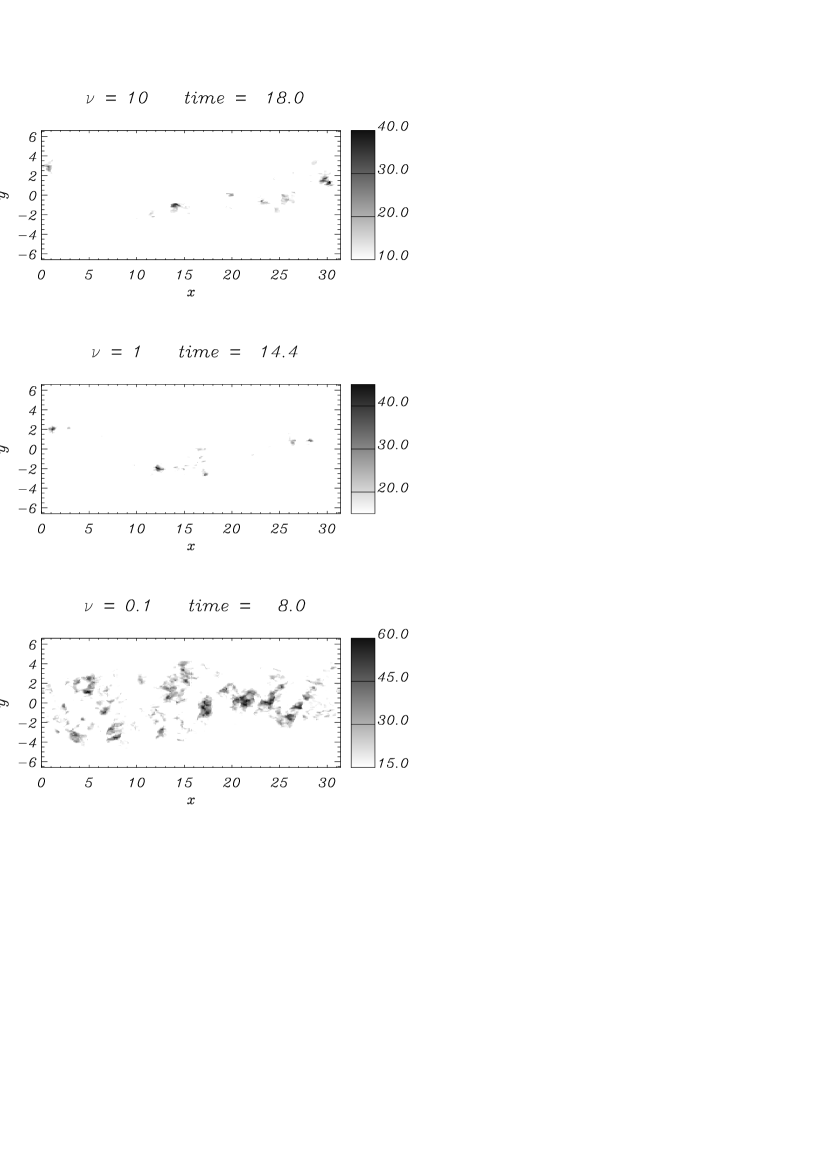
Figure 7: High velocity structures in the ambient medium, integrated over the $z$ direction.

Considering the time evolution of the mass distribution, we can deduce the temporal variation of the break velocity and of the spectral index (Fig. 5) from the temporal variation of the distribution of the average velocity with radius. In fact, comparing the two curves in Fig. 6 referring to the light jet case at times $t=16$ and $t=18$ (solid lines), we find that the maximum velocity value decreases with time, as well as the “break” value where the distribution of velocity with radius changes its slope ($\langle V\rangle\approx 2,\ t=16;\ \langle V\rangle\approx 1,\ t=18$). This explains the decrease in the break velocity with time, which is a common trend in all the studied cases (Fig. 5, panel b)). Moreover, comparing the slope of the average velocity profile at time $t=16$ with the one at time $t=18$ in the low velocity range, between $2a$ and $\sim 3a$ (Fig. 6), we note that the velocity distribution at time $t=18$ is flatter since more material has been accelerated at larger distances from the outflow axis. This implies a steepening of the mass distribution at low velocities, according to Eq. 1, and this is indeed what we see in the light and equal density jet cases (Fig. 5, panel a)).

Although the average velocity has the smooth profile shown in Fig. 6, the actual distribution can however show high velocity peaks, which may be correlated with the so called “EHV bullets”. We have marked the material moving at $V>40$ km s^-1 and integrated over the $z$ direction. The resulting images are displayed in Fig. 7. The figure shows that turbulent entrainment is able to accelerate “bullets” of material at high velocities and these are found within a few radii from the jet axis.

4.3 Collimation

Observational data on molecular outflows show that the flow collimation increases with flow velocity. Moreover, the blue-shifted and red-shifted lobes are generally well separated, especially at high velocities.

Figure 8: Distribution, in four different velocity intervals, of the ambient medium mass with respect to the angle $\theta$ between the flow velocity and the initial jet axis. These plots concern the light jet case, at time $t=18$

To verify whether these features are reproduced in our calculations, we considered at each grid point the angle $\theta$ between the outflow velocity and the initial jet axis. Smaller $\theta$ imply more collimated material. We divided the observed velocity range in four intervals, and for each of them we calculated the distribution of the ambient material mass with respect to $\theta$. One example of the distributions that we obtained is shown in Fig. 8, for the light jet case, at time $t=18$.

At low velocity the flow angle is distributed over a wide interval, and thus the flow is poorly collimated. The material moving at higher velocities moves at smaller angles respect to the initial flow axis, and is thus more collimated, in agreement with observations. This behavior is observed in all the studied cases, although a jet moving in a denser environment accelerates a more collimated outflow, while dense jets accelerate less collimated outflows. This trend can be inferred from Table 1 where we report the value of the angle $\theta$ within which is contained 90% of the ambient mass whose velocity lies in one of the four intervals defined in Fig. 8, at three significative times for the three cases. The variation with time is in any case quite small.

	$\nu=10$	$\nu=1$	$\nu=0.1$
	$time=18$	$time=18$	$time=12$
$2<V<10$ km s-1	88∘	101∘	124∘
$10<V<20$ km s-1	48∘	59∘	96∘
$20<V<35$ km s-1	36∘	36∘	48∘
$V>35$ km s-1	24∘		30∘

Table 1: Angle containing 90% of the ambient mass moving with velocity in the selected ranges, for the three cases, at three significative times.

Figure 9: Ratio between the mass of blue-shifted and red-shifted material, in the blue-shifted lobe, for outflows moving at an angle of $75^{\circ}$ (upper panel) and $60^{\circ}$ (lower panel) respect to the line of view, versus the flow velocity. The solid, dashed and dot-dashed lines refer, respectively, to the light, equal-density and heavy jet cases.

We evaluate now how these results compare with the observations regarding the overlapping of blue-shifted and red-shifted emission in molecular outflows.

This obviously depends on the angle $\psi$ between the line of sight and the flow axis (coincident with our $x$ axis) and we choose for our calculation two values for this angle, i.e. $\psi=75^{\circ}$ and $\psi=60^{\circ}$. For these two angles we compute the ratio of the blue-shifted (positive velocity along the line of sight) to the red-shifted (negative velocity along the line of sight) mass. In Fig. 9 we plot this ratio as a function of velocity. We notice that the ratio increases as this angle diminishes; when the flow is more directed towards the observer, in fact, only the material moving with large angles respect to the flow axis (i.e. the loosely collimated material) will appear red-shifted.

From our results we notice that the contrast ratio between blue-shifted and red-shifted material increases with velocity (again, the faster material is the more collimated one), in agreement with the data of, eg. Lada & Fich (1996). The contrast ratio, at all velocities, is higher for outflows driven by light jets, compared to outflows driven by equal density and heavy jets. In Fig. 9 we plot the trends for three selected times, and this is possible since we did not notice significant differences in the values and trends of the contrast ratios at different evolutionary times.

4.4 Acceleration and dissociation

One problem of the prompt entrainment mechanism for the acceleration of molecular outflows, is that as ambient medium is accelerated by the passage of a bow shock, it is also dissociated (Downes & Ray 1999), and thus, although the bow shock is very efficient in transferring momentum, most of it goes to atomic material and the effective fraction of momentum transfered by the jet to molecular material is low.

Figure 10: Distribution of the ambient accelerated mass as a function of its temperature, for different times, and for the light jet case.

In our case we cannot discuss molecular dissociation, since we did not include in our computations all the physics related to molecular formation and dissociation, and to molecular radiative losses. However it is possible to have a feeling of what the situation would be, by considering the temperature of the accelerated material. We limit the discussion to the light jet case: since we start from a configuration where the jet is in pressure equilibrium with the ambient medium, in the $\nu=10$ case the initial external temperature is $1/10$ of the initial jet temperature (i.e. $T_{ext}=1000$ K), while in the other cases the ambient medium is hotter from the beginning of the calculations and cannot be molecular.

In Fig. 10 we plot the distribution of the accelerated ambient material (i.e. external material with velocity $V>2$ km s^-1) with temperature; we note that at intermediate times (eg. $t=10,12,14$) a fraction of the ambient material is heated, and this is consistent with the fact that at this stage strong shocks are driven by the jet into the external medium. As shocks become weaker and disappear, the temperature of the accelerated ambient medium decreases. At all times, however, the largest fraction of accelerated material maintains a temperature not too different from the initial value. We can therefore expect that the ambient medium accelerated through turbulent entrainment at the jet surface remains mostly molecular.

5 Summary and Conclusions

We have shown that turbulent mixing in Kelvin-Helmholtz unstable jets is a very efficient mechanism of momentum transfer from the jet to the ambient medium: at the final stages of the evolution, up to 95% of the jet momentum has been transfered to entrained ambient material; since the momentum carried by parsec-scale YSO jets is found to be comparable to the momentum of typical molecular outflows, we infer that this mechanism alone can be invoked to explain the observed outflows. Moreover, opposite to what happens in bow-shock accelerated material, the temperature of the accelerated ambient medium remains low, and thus momentum is actually acquired by molecular material.

The transverse size of the outflows that are generated in this way is located at the lower end of the observed range, and our length to width ratio is too high with respect to the average value for molecular outflows but it is similar to that of highly collimated molecular outflows such as, for example NGC 2264G, Mon R2 and RNO43.

An interesting feature of our model is that it reproduces the observed distribution of mass with velocity: it has the form of a power law $M(v)\propto v^{\gamma}$, with a break at high velocities. The shape of the distribution and the values of the spectral index and of the break velocity are particularly well reproduced by the case in which a light jet is moving into a denser environment. The most powerful observed molecular outflows are located in the inner regions of molecular clouds, where the ambient medium is often so dense that the optical jets are completely obscured. It is thus plausible that in these cases the atomic jets are much lighter than the environment, as implied by our model. Conversely, bright optical jets coming out of the parent clouds, that would be probably denser than the surrounding ambient material, are accompanied by very weak molecular outflows, if any (HH 34 and HH 1-2, Chernin & Masson 1995). One exception is the bright optical jet HH 111, which is associated to a powerful molecular outflow (Cernicharo & Reipurth 1996). However, also in this case, the blueshifted jet breaking through the surface of the cloud is accompanied by a weaker molecular outflow with respect to the redshifted lobe surrounding the optically obscured counter-jet (Reipurth & Olberg 1991).

As far as the distribution of velocity with distance from the source is concerned, we could not reproduce the observed trend: we found that the average velocity of the outflow decreases with time (and thus with distance from the source, although only qualitative considerations can be performed on quantities requiring a translation from a temporal to a spatial approach), and this behavior is opposite to the observed “Hubble Law”. To explain the increase in velocity with distance from the source, many possibilities have been invoked: in the frame of the steady state model, Stahler (1994) inferred from analytical calculations that the Hubble law was a consequence of material with progessively higher velocities coming into view at greater distances from the star. The Hubble law could possibly be due to a decreasing density of the ambient medium (Padman et al. 1997), although, more probably, high velocities at the head of the flow are actually due to the presence of the bow shock that accelerates ambient material through prompt entrainment.

The collimation and bipolarity properties of the outflows generated with Kelvin Helmholtz induced turbulent entrainment fit very well the observations: the flow collimation increases with velocity, and there is a clear separation of the blue-shifted and red-shifted material, which increases as well with velocity. An example of a molecular outflow for which this behavior has been studied in detail is NGC 2264G, Lada & Fich (1996).

Since these preliminary results are encouraging, future work will analyze the combined effects of the two mechanisms, the turbulent entrainment at the jet surface and the prompt entrainment at the bow shock, studying the propagation of the jet’s head in space, and contemporarily the spatial growth of the Kelvin-Helmholtz unstable modes in the jet body.

Acknowledgments: The calculations have been performed on the Cray T3E at CINECA in Bologna, Italy, thanks to the support of CNAA. This work has been supported in part by the DOE ASCI/Alliances grant at the University of Chicago. M.M. acknowledges the CNAA 3/98 grant.

6 References

Bachiller, R., 1996, Ann.Rev.Astron.Astrophys 34, 111

Bally, J., Devine, D., 1994, ApJ Lett. 428, 65

Bodo, G., Massaglia, S., Ferrari, A., Trussoni, E., 1994, A&A 283, 655

Bodo, G.,Massaglia, S., Rossi, P., Rosner, R., Malagoli, A., Ferrari, A., 1995, A&A 303, 281

Bodo, G., Rossi, P., Massaglia, S., Ferrari, A., Malagoli, A., Rosner, R., 1998, A&A 333, 1117

Cabrit, S., Raga, A., Gueth, F., 1997, in “Herbig-Haro Outflows and the Birth of Low Mass Stars”, B. Reipurth & C. Bertout eds., IAU Symposium No. 182, Kluwer Academic Publishers, 163

Cernicharo, J., Reipurth, B., 1996, ApJ 460, L57

Chernin, L.M., Masson, C.R., 1995A, ApJ 455, 182

Chernin, L.M., Masson, C.R., 1995B, ApJ 443, 181

Davis, C.J., Eisloeffel, J., Ray, T.P., Jenness, T., 1997, A&A 324, 1013

Downes, T.P., Ray, T.P., 1999, A&A 345, 977

Fukui, Y., Iwata, T., Mizuno, A., Bally, J., Lane, A.P., 1993, in “Protostars and Planets III”, E.H. Levy & J.I. Lunine eds., University of Arizona Press, Tucson, 603

Lada, C.J., 1985, Ann.Rev.Astron.Astrophys 23, 267

Lada, C.J., Fich, M., 1996, ApJ 459, 638

Lizano, S., Heiles, C., Rodriguez, L.F., Koo, B., Shu, F.H., Hasegawa, T., Hayashi, S., Mirabel, I.F., 1988, ApJ 328, 763

Margulis, M., Lada, C.J., Hasegawa, T., Hayashi, S., Hayashi, M., Kaifu, N., Gatley, I., Greene, T.P., Young, E.T., 1990, ApJ 352, 615

Masson, C.R., Chernin, L.M., 1992, ApJ Lett 387, 47

Meyers-Rice, B.A., Lada, C.J., 1991, ApJ 368, 445

Micono, M., Massaglia, S., Bodo, G., Rossi, P., Ferrari, A., 1998, A&A 333, 989

Micono, M., Bodo, G., Massaglia, S., Rossi, P., Ferrari, A., Rosner, R., 2000, A&A, in press

Moriatry-Schieven, G.H., Snell, R.L., 1988, ApJ 332, 364

Moriatry-Schieven, G.H., Hughes, V.A., Snell, R.L., 1989, ApJ 347, 358

Padman, R., Bence, S., Richer, J., 1997, in “Herbig-Haro Outflows and the Birth of Low Mass Stars”, B. Reipurth & C. Bertout eds., IAU Symposium No. 182, Kluwer Academic Publishers, 123

Parker, N.D., Padman, R., Scott, P.F., 1991, MNRAS 252, 442

Raga, A., Binette, L., Cantó, J., 1990, ApJ 360, 612

Reipurth, B., Olberg, M., 1991, A&A 246, 535

Richer, J.S., Hills, R.E., Padman, R., 1992, MNRAS 254, 525

Rodriguez-Franco, A., Martin-Pintado, J., Wilson, T.L., 1999, A&A 351, 1103

Rossi P., Bodo, G., Massaglia, S., Ferrari, A., 1997, A&A 321, 672

Stahler, S.W., 1994, ApJ 422, 616

Taylor, S.D., Raga, A.C., 1995, A&A 296, 823

Uchida, Y., Kaifu, N., Shibata, K., Hayashi, S., Hasegawa, T., Hamatake, H., 1987, Publ. of the Astron. Soc. of Jap., 39, 907