A simple model of the hierarchical formation of galaxies

Abstract

We develop a simple, fast and predictive model of the hierarchical formation of galaxies which is in quantitative agreement with observations. Comparing simulations with observations we place constraints on the density of the universe and on the power spectrum of density fluctuations.

1 Introduction

Simulations of galaxy formation usually start with a set of gravitating point particles with given initial conditions which are then stepped forward in time using huge computer resources. Here we consider a complementary approach with a density distribution that is continuous instead of discrete. The model is presented in Section 2 and compared with observations in Section 3. Conclusions are collected in Section 4.

2 Model of galaxy formation

2.1 The hierarchical formation of galaxies

Let us study linear departures from a critical universe dominated by non-relativistic dark matter.[1] We consider a cube of side $L(t)=a_{c}(t)L_{0}$ and expand the density in this cube in a Fourier series. For growing modes with $\delta_{c}\ll 1$ we define the linear approximation of the density of the universe as follows:

$$\rho_{lin}(\vec{x},t,I) \equiv \frac{1}{6\pi Gt^{2}}\{1+\delta_{c}(\vec{x},t)\}\equiv\frac{\rho^{\prime}_{c0}}{a_{c}^{3}}\{1+\delta_{c}(\vec{x},t)\}$$ (1)

$$= \frac{\rho^{\prime}_{c0}}{a_{c}^{3}}\left\{1+\Delta(\Omega_{0})a_{c}+\sum_{\vec{k},0<k\leq k_{I}}|\delta_{\vec{k}}|a_{c}\cdot\exp\left[i\frac{\vec{k}\cdot\vec{x}}{a_{c}}+i\varphi_{\vec{k}}\right]\right\}$$

where $t$ is the age of the universe, the subscript $0$ denotes present day values, $\rho^{\prime}_{c0}\equiv\omega(\Omega_{0})\rho_{c0}$, $\rho_{c0}\equiv 3H_{0}^{2}/(8\pi G)$ is the critical density, and $a_{c}(t)\equiv(t/t_{0})^{2/3}$. $\varphi_{\vec{k}}$ are random phases. Until Section 3.7 we will take the cosmological constant $\Lambda=0$. The functions $\Delta(\Omega_{0})$ and $\omega(\Omega_{0})=[2/(3H_{0}t_{0})]^{2}$ are given in Tables 1 and 2. The sum of the Fourier series is over comoving wavevectors that satisfy periodic boundary conditions:

$$\vec{k}=\frac{2\pi}{L_{0}}(n\hat{\imath}+m\hat{\jmath}+l\hat{k})$$ (2)

where $n,m,l=0,\pm 1,\pm 2,\pm 3\cdots$ and $1\leq[n^{2}+m^{2}+l^{2}]^{1/2}\leq I$. The density in Equation (1) is due to Fourier components up to wavevectors of magnitude $k_{I}\equiv 2\pi I/L_{0}$. Note that the critical density $\rho_{c}=\rho_{c0}/a_{c}^{3}$ is proportional to $a_{c}^{-3}$, the density contrast $\delta_{c}$ grows in proportion to $a_{c}$, and the “wavelengths” $\lambda=2\pi a_{c}/|\vec{k}|$ of the Fourier components stretch in proportion to $a_{c}$ (we use the word “wavelength” even though (1) does not describe a wave). Our convention for Fourier transforms is:

$$\delta_{\vec{k}}=\frac{1}{V}\int\delta_{c}(\vec{x},t_{0})\exp(-i\vec{k}\cdot\vec{x})d^{3}\vec{x}$$ (3)

$$\delta_{c}(\vec{x},t_{0})=\sum_{\vec{k}}\delta_{\vec{k}}\exp(i\vec{k}\cdot\vec{x})=\frac{V}{(2\pi)^{3}}\int\delta_{\vec{k}}\exp(i\vec{k}\cdot\vec{x})d^{3}\vec{k}$$ (4)

where $V\equiv L_{0}^{3}$. We take the power spectrum of density fluctuations (as defined in (1) and extrapolated to today in the linear approximation) to be of the form

$$P(k)\equiv\frac{V}{(2\pi)^{3}}|\delta_{\vec{k}}|^{2}=\frac{Aw^{n}}{(1+\eta w+w^{2})^{2}}$$ (5)

with $w\equiv k/k_{eq}$. Note that $P(k)\propto k^{n}$ at $k\ll k_{eq}$ and $P(k)\propto k^{n-4}$ at $k\gg k_{eq}$. The scale invariant Harrison-Zel’dovich spectrum has $n=1$. The power spectrum $P(k)$ is normalized such that

$$\frac{1}{V}\int_{V}\delta_{c}^{2}(\vec{x},t_{0})d^{3}\vec{x}=\int P(k)d^{3}\vec{k}=\sum_{\vec{k}}|\delta_{\vec{k}}|^{2}.$$ (6)

$\Omega_{0}$	$\Delta(\Omega_{0})$	$\Omega_{0}$	$\Delta(\Omega_{0})$
$0.2$	$-1.645$	$1.0$	$0.000$
$0.3$	$-1.066$	$1.2$	$0.104$
$0.5$	$-0.517$	$1.5$	$0.216$
$0.7$	$-0.239$	$2.0$	$0.341$

Table 1: Function $\Delta(\Omega_{0})$ for zero cosmological constant.

$\Omega_{0}$	$\omega(\Omega_{0})$	$\Omega_{0}$	$\omega(\Omega_{0})$
$0.2$	$0.620$	$1.0$	$1.000$
$0.3$	$0.679$	$1.2$	$1.078$
$0.5$	$0.783$	$1.5$	$1.189$
$0.7$	$0.875$	$2.0$	$1.364$

Table 2: Function $\omega(\Omega_{0})$ for zero cosmological constant.

Equation (1) corresponds to the linear approximation valid when $\delta_{c}\ll 1$. Exact solutions can be obtained at peaks of the density fluctuations (assuming peaks of spherical symmetry and negligible pressure). When $\delta_{c}=1.06$ in the linear approximation (which has already broken down), the exact solution is $\delta=4.55$ and the density fluctuation has reached maximum expansion. When $\delta_{c}=\delta_{m}=1.69$ in the linear approximation, the exact solution $\delta$ diverges, the density fluctuation has collapsed and, in our model, a galaxy has formed.

The generation of galaxies on a computer at a given expansion parameter $a_{c}$ proceeds as follows (see Figure 1). We begin with the largest possible galaxy with $I=2$. We scan the cube searching for maximums of $\delta_{c}(\vec{x},t)$. If the maximum at $\vec{x}$ is not “occupied” by a galaxy (see below), and if $\delta_{c}(\vec{x},t)\geq\delta_{m}=1.69$, we generate a new galaxy at $\vec{x}$ with the characteristics listed below. We increase $I\rightarrow I+1$ and repeat the calculation to form galaxies of a smaller generation, and repeat this process up to $I=I_{max}$ corresponding to the smallest galaxies that we wish to generate.

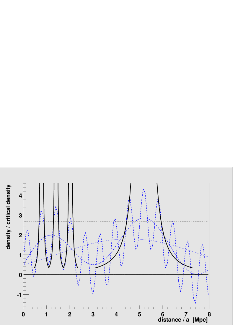
Figure 1: The hierarchical formation of galaxies. Dashed lines: Sum of one, two and three Fourier components of the density in the linear approximation. When the density in the linear approximation reaches the dotted line a galaxy forms. Full lines: Halos of several galaxies with density run $\rho\propto r^{-2}$. As larger wavelengths reach the dotted line, larger galaxies form “swallowing” galaxies of previous generations. The peculiar displacements of the galaxies have not yet been applied.

Note that as time goes on, larger and larger distance scales $\lambda_{I}=2\pi a_{c}/k_{I}$ become non-linear and new galaxies of larger mass form, “swallowing” up galaxies of previous generations. Study Figure 1 again. Galaxy formation is therefore an ongoing hierarchical process: today’s galaxy clusters are the seeds of tomorrow’s galaxies.

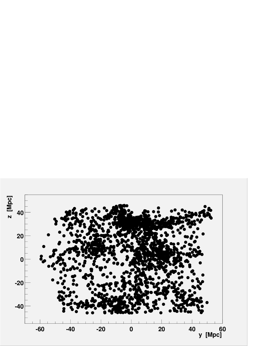
Figure 2: Scatter plot of $y$ vs. $z$.

2.2 Galaxy characteristics

We assume that the barionic matter discipates energy and falls to the bottom of the halo potential wells with density run $\rho\propto r^{-2}$[2]. The galaxies generated at “generation” $I$ have the following properties regarded as approximate descriptions of complex phenomena. Luminous and total (luminous $+$ dark) radius:

$$\frac{\Omega_{0}}{\Omega_{lum}}R_{lum}=R=\frac{\lambda_{I}}{2}=\frac{\pi a_{c}(t)}{k_{I}},$$ (7)

(see Figure 1); luminous and total mass:

$$\frac{\Omega_{0}}{\Omega_{lum}}M_{lum}=M\approx\frac{4}{3}\pi R^{3}\Omega(t)\rho_{c}(t),$$ (8)

velocity of circular orbits (if spiral):

$$v_{c}=\sqrt{\frac{GM}{R}},$$ (9)

or 3-dimensional velocity dispersion (if elliptical)[2]:

$$v_{rms}\equiv\sqrt{\langle v^{2}\rangle}\equiv\sqrt{3}\sigma=\sqrt{\frac{3GM}{2R}},$$ (10)

peculiar velocity[1]:

$$\vec{v}_{pec}(\vec{x},t)\approx\sum_{\vec{k},0<k\leq k_{I-1}}\frac{2i\vec{k}a_{c}^{2}|\delta_{\vec{k}}|}{3k^{2}t}\cdot exp\left[i\frac{\vec{k}\cdot\vec{x}}{a_{c}}+i\varphi_{\vec{k}}\right],$$ (11)

(the sum is over $\vec{k}$ up to $k=k_{I-1}$ while the peculiar motion given by (13), $|\vec{x}_{pec}|$, is less than $\lambda/2=\pi a_{c}/k$); and peculiar acceleration:

$$\vec{g}_{pec}(\vec{x},t)\approx\frac{\vec{v}_{pec}(\vec{x},t)}{t}.$$ (12)

What do we mean by “occupied”? To generate a galaxy of total radius $R$ at position $\vec{x}$ we require that the distance from $\vec{x}$ to already generated galaxies of radius $R^{\prime}$ be greater than $R^{\prime}+0.7R$. The factor $\approx 0.7$ was included to approximately fill space.

Finally, after generating all galaxies, we correct their positions $\vec{x}$ by their peculiar motions

$$\vec{x}_{pec}\approx\int_{0}^{t}\vec{v}_{pec}(\vec{x},t^{\prime})\frac{a_{c}(t)}{a_{c}(t^{\prime})}dt^{\prime}\approx\frac{3}{2}\vec{v}_{pec}(\vec{x},t)t.$$ (13)

This step is necessary in order to obtain the galaxy-galaxy correlation. This completes the presentation of the model.

Figure 3: Scatter plot of $M$ vs. $v_{c}$ to test the Tully-Ficher relation.

2.3 The simulations

Our simulations are limited by computer resources (one $500$ MHz, $32$ bit processor). Therefore, we fix $L_{0}=92$Mpc. Even then the contributions to $\rho_{lin}$ from Fourier components with $I=1$ and edge effects are non-negligible. More realistic simulations require a larger $L_{0}$. We fix $h_{0}=0.6$, $\eta=2.04$ and $k_{eq}=0.155$Mpc${}^{-1}\cdot\Omega_{0}h_{0}^{2}\cdot\{3.36/N_{eff}\}^{1/2}$. This value of $k_{eq}$ corresponds to a distance to the horizon equal to $\approx 0.5\lambda_{eq}$ at the time $t_{eq}$ when the densities of radiation and matter were equal. $N_{eff}$ is the effective value of $N_{b}+\frac{7}{8}N_{f}$, where $N_{b}$ ($N_{f}$) is the number of boson (fermion) degrees of freedom. $N_{eff}=3.36$ for three light neutrino species. The values of $k_{eq}$ and $\eta$ were obtained from a fit to the “CHDM” model of reference [3] which is in agreement with observations.

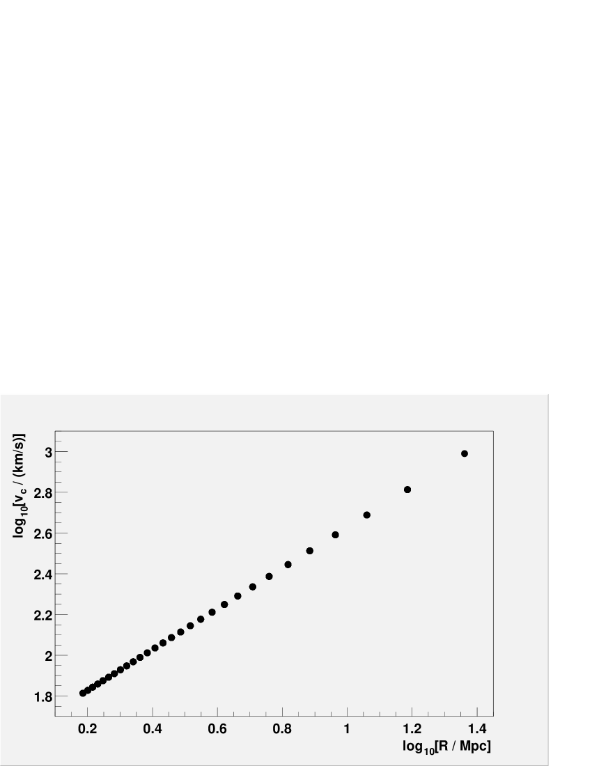
Figure 4: Scatter plot of $R$ vs. $v_{c}$ to test the Samurai relation.

3 Comparison with observations

The results of the model are presented and compared with observations in Figures 2 to 9 and Table 4. These figures correspond to the simulation with $\Omega_{0}=1.0$, $n=1.00$ and $A=1706$Mpc³. Explanations follow.

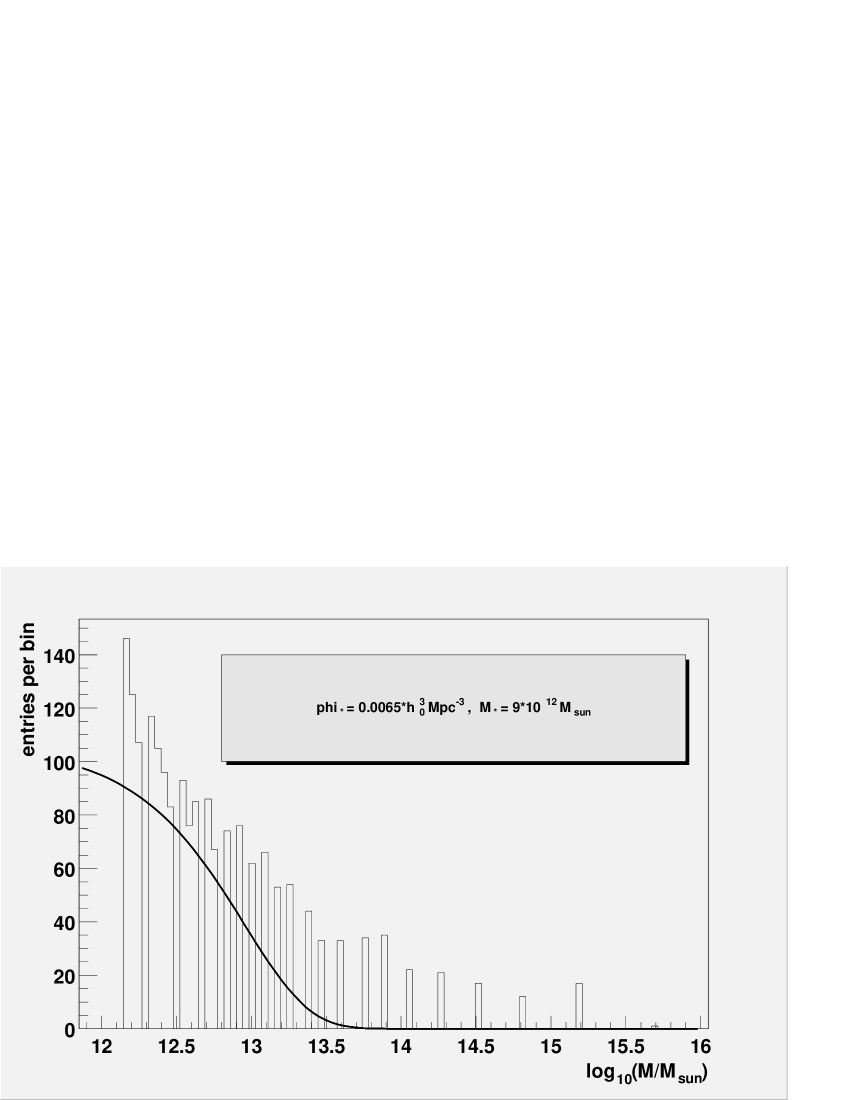
Figure 5: Histogram of $\log_{10}(M)$ to test the Schechter distribution.

3.1 Tully-Fisher, Faber-Jackson and Samurai relations

The model satisfies $M_{lum}\propto v_{c}^{3}\propto v_{rms}^{3}$, which, if light traces mass, is in reasonable agreement with the Tully-Fisher relation for spiral galaxies ($L\propto v_{c}^{\mu}$ with $\mu\approx 4$[4] for the infrared luminosity and $\mu\approx 2.4$ to $2.8$ for the blue luminosity), or the Faber-Jackson relation for elliptical galaxies ($L\propto v_{rms}^{\mu}$ with $\mu=4\pm 1$[4]). $L$ is the galaxy absolute luminosity. The model satisfies $R_{lum}\propto v_{rms}\propto v_{c}$, which is in reasonable agreement with the Samurai relation for elliptical galaxies ($R_{lum}\propto v_{rms}^{\xi}$ with $\xi\approx 1.2$ to $1.3$). See Figures 3 and 4. Elliptical galaxies satisfy the following relation with “remarkably small”[4] scatter: $v_{rms}\propto L^{0.62}R_{lum}^{-0.50}\propto M_{lum}^{0.50}R_{lum}^{-0.50}$.[4] This relation is in excellent agreement with our model.

The model satisfies the following useful relations at present:

$$\left(\frac{R_{lum}}{1\textrm{Mpc}}\right)=1.4\Omega_{0}^{-3/2}\Omega_{lum}h_{0}^{-1}\left(\frac{v_{c}}{100\textrm{km}\cdot\textrm{s}^{-1}}\right),$$ (14)

$$\left(\frac{M_{lum}}{M_{sun}}\right)=3.3\cdot 10^{12}\Omega_{0}^{-3/2}\Omega_{lum}h_{0}^{-1}\left(\frac{v_{c}}{100\textrm{km}\cdot\textrm{s}^{-1}}\right)^{3},$$ (15)

Both equations are in reasonable agreement with observations if the density of matter in optically bright baryons is $\Omega_{lum}\approx 0.005$.

3.2 The Schechter distribution

The observed galaxy luminosity distribution is given by the Schechter relation.[4] Assuming that light traces mass, we obtain the following total (luminous $+$ dark) mass distribution of galaxies:

$$\frac{dn}{d\ln(M)}\approx\phi_{*}\exp\left(-\frac{M}{M_{*}}\right)$$ (16)

where $dn$ is the number of galaxies per unit volume with total mass between $M$ and $M+dM$, $\phi_{*}=0.010\exp(\pm 0.4)h_{0}^{3}$Mpc^-3 and $M_{*}=M_{lum*}\Omega_{0}\Omega_{lum}^{-1}=2.8\cdot 10^{13}\exp(\pm 0.4)\Omega_{0}h_{0}^{-1}M_{sun}$.[4] The corresponding velocity of circular orbits is $v_{c*}$. See Figures 5 and 6.

We choose galaxies of total mass $M_{*}$ to be of “generation” $I\approx 10$. Then our simulations require $L_{0}\approx I(6M_{*}/\pi\Omega_{0}\rho_{c0})^{1/3}$. We therefore set $L_{0}=92$Mpc as indicated above. We also set $I_{max}=30$ so that galaxies are generated down to a mass $\approx M_{*}/27$. Galaxies with less mass contribute negligibly to the density of the universe and the computer resources needed to generate them become prohibitive. The simulations then probe the power spectrum in the wavevector range $0.1$Mpc${}^{-1}\lesssim k<2.0$Mpc^-1.

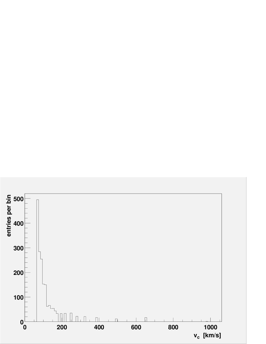
Figure 6: Histogram of the velocity of circular orbits $v_{c}$.

3.3 Galaxy-galaxy correlation

The observed joint probability of finding two galaxies in two volume elements separated by $r$ is

$$dP\propto\left[1+\left(\frac{r_{0}}{r}\right)^{\gamma}\right]dV_{1}dV_{2}$$ (17)

with $\gamma=1.77\pm 0.04$ and $r_{0}=(5.4\pm 1.0)h_{0}^{-1}$Mpc.[4] Due to the linear approximation of $\vec{x}_{pec}$ we expect agreement with observations to break down at small $r$. See Figure 7.

3.4 Fluctuation in galaxy counts

The observed fluctuation in galaxy counts in randomly placed spheres of radius $r$ is[4]

$$\frac{\left<\delta N\right>_{rms}}{\left<N\right>}=1.35\left(\frac{r_{0}}{r}\right)^{\gamma/2}=0.84\pm 0.17$$ (18)

for $r=9.2h_{0}^{-1}\textrm{Mpc}=92\textrm{Mpc}/6$ which is a convenient radius in view of our simulation volume.

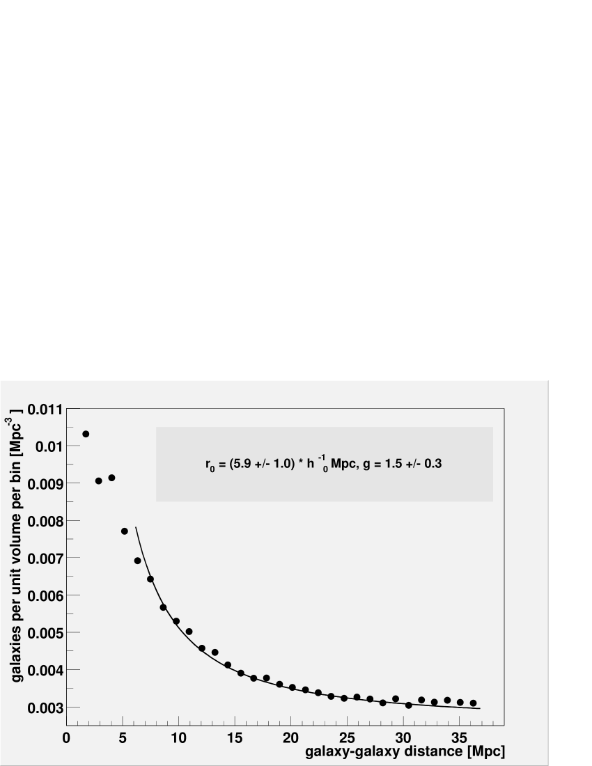
Figure 7: Histogram of distances between galaxies to test the galaxy-galaxy correlation.

3.5 Fluctuations of the Cosmic Microwave Background

The Cosmic Microwave Background (CMB) radiation propagates freely since matter and radiation decoupled at $T_{dec}\approx 3000$K, or at $a_{dec}\equiv(1+z_{dec})^{-1}\approx 1100^{-1}$. The relation between the comoving length at decoupling (or at any time with $a\ll 1$) with the corresponding angle today is[4]

$$R_{0}=\frac{2c}{\Omega_{0}H_{0}}\theta=\frac{1.74\textrm{Mpc}}{\Omega_{0}h_{0}}\left(\frac{\theta}{1^{\prime}}\right)$$ (19)

Fluctuations on scales $\theta<6^{\prime}$ are erased due to the thickness of the last scattering surface. The size of the horizon at decoupling, $3ct_{dec}$, corresponds to $\theta_{dec}\approx 1.7^{o}$. The size of the horizon at $t_{eq}$, $\approx 2ct_{eq}$, corresponds to $\theta_{eq}\approx 0.3^{o}$.

We consider the root-mean-square fluctuation of the temperature of the CMB on angular scales $\theta\gg 1.7^{o}$, i.e. fluctuations that entered the horizon after the decoupling of matter and radiation. On these large scales

$$P(k)=A(k/k_{eq})^{n}.$$ (20)

We use a “window function”[5]

$$W(r)=\exp\left(-\frac{r^{2}}{2r_{W}^{2}}\right)$$ (21)

which smoothly defines a volume

$$V_{W}\equiv\frac{4}{3}\pi r_{s}^{3}=4\pi\int_{0}^{\infty}r^{2}W(r)dr=(2\pi)^{3/2}r_{W}^{3}$$ (22)

Then the mean-square fluctuation of mass in randomly chosen windows of volume $V_{W}$ is:

$$\left<\frac{\delta M}{M}\right>_{rms}^{2} \equiv \frac{1}{V}\int_{V}d^{3}\vec{x}\left[\frac{1}{V_{W}}\int_{V_{W}}d^{3}\vec{r}\delta_{c}(\vec{x}+\vec{r})W(\vec{r})\right]^{2}$$ (23)

$$= \frac{V}{2\pi^{2}}\int_{0}^{\infty}\left|\delta_{\vec{k}}\right|^{2}\exp\left(-k^{2}r_{W}^{2}\right)k^{2}dk$$

at early times, i.e. $\Omega\approx 1$. For the power spectrum (20) in the range of interest of $n$ we obtain approximately

$$\left<\frac{\delta M}{M}\right>_{rms}^{2}\approx\frac{2\pi A}{k_{eq}^{n}r_{W}^{n+3}}$$ (24)

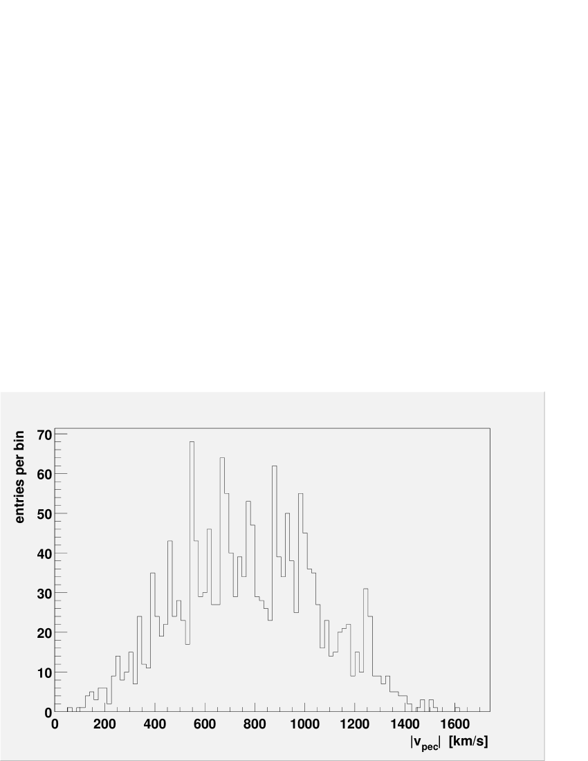
Figure 8: Histogram of the absolute peculiar velocities of galaxies.

The fluctuation of the temperature of the CMB radiation is given by the Sachs-Wolfe effect[4, 5, 6]. To obtain an analytic expression we use the prescription:

$$\left<\frac{\delta T}{T}\right>_{rms,\theta}\approx\left<\frac{\delta M}{M}\right>_{rms,H,\theta}$$ (25)

where $\left<\delta M/M\right>_{rms,H,\theta}$ is the root-mean-square fluctuation of mass on the scale corresponding to angle $\theta$ when that mass crossed inside the horizon. The prescription (25) is in agreement with numerical calculations[3, 4]. From (25), (24), (22), (19) for $r_{s}$, and replacing $A^{1/2}$ by the amplitude at horizon crossing $a_{cH}A^{1/2}\equiv a_{H}f(\Omega_{0})A^{1/2}=\theta^{2}\Omega_{0}^{-1}f(\Omega_{0})A^{1/2}$, and substituting numerical values, we finally obtain

$$\left<\frac{\delta T}{T}\right>_{rms,\theta}\approx\Omega_{0}^{\frac{1}{2}}\cdot f(\Omega_{0})\left[\frac{A}{43\textrm{Mpc}^{3}}\right]^{\frac{1}{2}}\left[\frac{N_{eff}}{3.36}\right]^{\frac{n}{4}}\left[\frac{h_{0}^{n+3-2n}}{598^{n+3}\theta^{n-1}}\right]^{\frac{1}{2}}$$ (26)

with $\theta$ in radians, and $f(\Omega_{0})=3(1-\Omega_{0}^{-1})/(5\Delta(\Omega_{0}))$. The published fluctuation of the temperature of the CMB is given in terms of the amplitudes of spherical harmonis $a_{\ell}\equiv\left<|a_{\ell}^{m}|\right>$[4]:

$$\left<\frac{\delta T}{T}\right>_{rms,\theta}=\frac{1}{T_{0}}\left[\sum_{\ell=2}^{\infty}\frac{2\ell+1}{4\pi}a_{\ell}^{2}\exp\left(-\theta^{2}\ell^{2}\right)\right]^{\frac{1}{2}}$$ (27)

for $\theta\ll 2\pi$.

Figure 9: Histogram of the component $v_{y}$ of the absolute peculiar velocity.

3.6 Peculiar velocities

The absolute peculiar velocities of galaxies with respect to the CMB, shown in Figures 8 and 9, have relatively large contributions from wavevectors $k\approx k_{eq}/\eta$ which are well beyond the range of our simulations. Furthermore, these absolute peculiar velocities are difficult to measure. We therefore define a local peculiar velocity in spheres of radius $r=9.2h_{0}^{-1}\textrm{Mpc}$:

$$\left<v_{pec}\right>_{rms}\equiv\left<\left[\frac{1}{N}\sum_{i=1}^{N}\left|\vec{v}_{pec,i}-\left<\vec{v}_{pec}\right>\right|^{2}\right]\right>^{\frac{1}{2}}$$ (28)

where $N$ is the number of galaxies in a sphere and the average is over all spheres. This local peculiar velocity can be estimated from the lengths of the “Fingers of God”.[4] See also [8].

$\left<\delta T/T\right>_{rms,\theta=0.1745}=(1.06\pm 0.04\pm 0.20)\cdot 10^{-5}$

$v_{c*}=(220\pm 50\pm 60)$km s-1

$\left<v_{pec}\right>_{rms}\approx(748\pm 150\pm 350)$km s-1

$\delta N/N=0.84\pm 0.17\pm 0.10$

$r_{0}=(5.4\pm 1.0\pm 2.8)h_{0}^{-1}$Mpc

$\gamma=1.77\pm 0.04\pm 0.54$

$\ln(\phi_{*}\cdot h_{0}^{-3}\cdot\textrm{Mpc}^{3})=-4.6\pm 0.4\pm 0.5$

Table 3: Benchmark data[4, 7, 8] used to define a $\chi^{2}$ to compare the model with observations. The first error is observational, and the second one includes theoretical errors, statistical errors of the simulations and errors of the fits. We add them in quadrature. All errors in this article are one standard deviation.

3.7 The cosmological constant

Until now we have set $\Omega_{\Lambda}=0$. Let us consider a low density spatially flat universe with $\Omega_{0}=0.3$ and $\Omega_{\Lambda}=0.7$. By numerical integration we obtain $H_{0}t_{0}=0.964$, $\omega=0.478$, $\Delta=0.0$, $\delta_{m}=1.85$ and $f=1.17$. The simulation then proceeds as before. The results are discussed in the next Section.

$\Omega_{0}$, $\Omega_{\Lambda}$ $\backslash$ $n$	$1.50$	$1.25$	$1.00$	$0.75$	$0.50$
$0.20$, $0.0$	$11.8$	$11.4$	*	*	*
$0.35$, $0.0$	$72.4$	$5.7$	$12.8$	*	*
$0.50$, $0.0$	$196.6$	$5.8$	$8.5$	**	*
$0.70$, $0.0$	$24.7$	$16.2$	$6.6$	$11.5$	*
$1.00$, $0.0$	$46.3$	$10.7$	$3.2$	$7.3$	$78.0$
$1.50$, $0.0$	$162.7$	$98.4$	$3.7$	$5.3$	$14.3$
$0.30$, $0.7$	$38.3$	$9.2$	$12.2$	*	*

Table 4: We compare the model with observations by giving the $\chi^{2}$ for $4$ degrees of freedom for several $\Omega_{0}$, $\Omega_{\Lambda}$ and $n$. The amplitude $A^{1/2}$ was obtained from COBE data[7] and Equation (26) for each pair $(\Omega_{0},n)$. Entries with a star are excluded because zero galaxies were generated. Entries with $\chi^{2}>9.5$ are excluded with $95\%$ confidence.

3.8 Constraints on $\Omega_{0}$, $n$ and $A$

To compare quantitatively the predictions of the model with observations we define a $\chi^{2}$ as indicated in Table 3. This $\chi^{2}$ has seven terms and the model has three parameters ($\Omega_{0}$, $n$ and $A$), so we are left with four degrees of freedom. We have excluded from $\chi^{2}$ the Tully-Fisher and Samurai parameters $\mu$ and $\xi$, which are well satisfied, because they are common to all simulations. The theoretical errors of $\delta N/N$, $\gamma$ and $r_{0}$ quoted in Table 3 are obtained from an estimate of the error of $\vec{v}_{pec}$ in the approximation (11), and the propagation of this error as determined from numerical simulations.

Several simulations are compared with observations in Table 4. For each pair ($\Omega_{0}$, $n$) we have obtained $A$ from COBE data (see Table 3) and Equation (26). Note that we obtain good quantitative agreement with observations for several pairs ($\Omega_{0}$, $n$).

The best simulation with $\Omega_{\Lambda}=0$ has $\chi^{2}=3.2$, the critical density $\Omega_{0}=1.0$, the scale invariant Harrison-Zel’dovich slope $n=1.00$, and $A=1706$Mpc³. This simulation has $2053$ galaxies, $M_{lum*}=9\cdot 10^{12}M_{sun}\Omega_{lum}\Omega_{0}^{-1}$, $v_{c*}=118$km/s, $\phi_{*}=0.0065h_{0}^{3}$Mpc^-3, $R_{lum*}=2.8$Mpc$\Omega_{lum}\Omega_{0}^{-1}$, $\left<v_{pec}\right>_{rms}=486$km/s, $\delta N/N=0.744$, $r_{0}=(5.9\pm 1.0)h_{0}^{-1}$Mpc, $\gamma=1.5\pm 0.3$ (these are errors of the fit), and a fraction of mass in galaxies $\epsilon=0.97$. Several distributions of this simulation are presented in Figures 2 to 9.

Some results of the simulations are shown in Tables 5 to 8.

$\Omega_{0}$, $\Omega_{\Lambda}$ $\backslash$ $n$	$1.50$	$1.25$	$1.00$	$0.75$	$0.50$
$0.20$, $0.0$	$3017$	$708$	$0$	$0$	$0$
$0.35$, $0.0$	$1929$	$2584$	$397$	$0$	$0$
$0.50$, $0.0$	$1444$	$2229$	$1866$	$22$	$0$
$0.70$, $0.0$	$1146$	$1765$	$2285$	$778$	$0$
$1.00$, $0.0$	$890$	$1398$	$2053$	$1937$	$194$
$1.50$, $0.0$	$846$	$1120$	$1635$	$2057$	$1550$
$0.30$, $0.7$	$1451$	$2277$	$1094$	$0$	$0$

Table 5: Number of galaxies in the simulations as a function of $\Omega_{0}$, $\Omega_{\Lambda}$ and $n$.

4 Conclusions

We have developed a simple, fast and predictive model of the hierarchical formation of galaxies. We obtain quantitative agreement with observations (within the limitations of the model, i.e. outside of the core of galaxy clusters). The only free parameters of the model are $\Omega_{0}$ and the power spectrum of density fluctuations, i.e. $n$ and $A$. The COBE observations determine $A$ as a function of $\Omega_{0}$ and $n$. The model provides insight into the hierarchical formation of galaxies, and is useful to study the onset of galaxy formation, the merging of galaxies, the redshift-luminosity distributions, and so forth, and to further constrain $\Omega_{0}$, $n$, $A$ and $N_{eff}$.

The model is robust for two reasons: i) Galaxies are not stepped forward in time so errors do not accumulate in time; and ii) Galaxies are placed where the exact solution for the density diverges. Weaknesses of the model are: i) Galaxy formation and merging in the model is step-wise rather than continuous; and ii) The peculiar velocities and displacements are calculated in the linear approximation. Therefore, we expect that the simple model will not reproduce the center of galaxy clusters in detail which are in the process of merging and have gone non-linear, nor will it predict correctly the galaxy-galaxy correlation at small separation.

Comparison of general galaxy observations with simulations determines, with $95\%$ confidence, that $\Omega_{0}>0.25$ and $1.1-0.3\Omega_{0}<n<1.4-0.2\Omega_{0}$ (assuming $\Omega_{\Lambda}=0$ and $N_{eff}=3.36$). The best simulation has a $\chi^{2}$ per degree of freedom equal to $3.2/4$ and corresponds to $\Omega_{0}=1.0$, $\Omega_{\Lambda}=0$ and $n=1.00$. A low density flat universe with $\Omega_{0}=0.3$ and $\Omega_{\Lambda}=0.7$ is still allowed. See Table 4 for details.

In summary, we have developed a simple, fast and powerful tool to study the large scale structure of the universe.

$\Omega_{0}$, $\Omega_{\Lambda}$ $\backslash$ $n$	$1.50$	$1.25$	$1.00$	$0.75$	$0.50$
$0.20$, $0.0$	$1.06$	$0.46$	*	*	*
$0.35$, $0.0$	$1.31$	$0.76$	$0.49$	*	*
$0.50$, $0.0$	$1.55$	$0.93$	$0.49$	**	*
$0.70$, $0.0$	$1.62$	$1.15$	$0.64$	$0.44$	*
$1.00$, $0.0$	$1.37$	$0.96$	$0.74$	$0.50$	$0.39$
$1.50$, $0.0$	$1.35$	$1.40$	$0.65$	$0.53$	$0.38$
$0.30$, $0.7$	$1.34$	$0.81$	$0.45$	*	*

Table 6: $\delta N/N$ as a function of $\Omega_{0}$, $\Omega_{\Lambda}$ and $n$. Entries with a star have zero galaxies.

$\Omega_{0}$, $\Omega_{\Lambda}$ $\backslash$ $n$	$1.50$	$1.25$	$1.00$	$0.75$	$0.50$
$0.20$, $0.0$	$568$	$234$	*	*	*
$0.35$, $0.0$	$916$	$428$	$204$	*	*
$0.50$, $0.0$	$1086$	$594$	$279$	**	*
$0.70$, $0.0$	$1254$	$761$	$382$	$192$	*
$1.00$, $0.0$	$1531$	$967$	$486$	$284$	$130$
$1.50$, $0.0$	$1668$	$1085$	$645$	$397$	$220$
$0.30$, $0.7$	$756$	$337$	$156$	*	*

Table 7: $\left<v_{pec}\right>_{rms}$ in km/s as a function of $\Omega_{0}$, $\Omega_{\Lambda}$ and $n$. Entries with a star have zero galaxies.

$\Omega_{0}$, $\Omega_{\Lambda}$ $\backslash$ $n$	$1.50$	$1.25$	$1.00$	$0.75$	$0.50$
$0.20$, $0.0$	$43$	$33$	*	*	*
$0.35$, $0.0$	$69$	$60$	$48$	*	*
$0.50$, $0.0$	$80$	$80$	$69$	**	*
$0.70$, $0.0$	$97$	$97$	$85$	$77$	*
$1.00$, $0.0$	$118$	$118$	$118$	$109$	$97$
$1.50$, $0.0$	$143$	$129$	$139$	$131$	$143$
$0.30$, $0.7$	$67$	$58$	$53$	*	*

Table 8: Velocity of circular orbits of $L_{*}$ galaxies, $v_{c*}$, in km/s as a function of $\Omega_{0}$, $\Omega_{\Lambda}$ and $n$. Entries with a star have zero galaxies.

References

- [1] S. Weinberg, “Gravitation and Cosmology”, Wiley (1972)
- [2] B. Hoeneisen, Jornadas en Ingeniería Eléctrica y Electrónica, 12, 62, Escuela Politécnica Nacional, Quito, Ecuador (1990); B. Hoeneisen and J. Mejía, Politécnica 18, No. 4, 39, Quito, Ecuador (1993); B. Hoeneisen, CIENCIA, Vol. 1, No. 1, 105, Quito, Ecuador (1998); B. Hoeneisen, “Thermal physics”, The Edwin Mellen Press(1993)
- [3] Eric Gawiser and Joseph Silk, Science, 280, 1405 (1998). Our conventions for differ by a factor .
- [4] P.J.E. Peebles, “Principles of Physical Cosmology”, Princeton University Press (1993)
- [5] Michael S. Turner, “Cosmology and Particle Physics” in “Intersection between Elementary Particle Physics and Cosmology”, Volume 1, edited by T. Piran and S. Weinberg, World Scientific (1984)
- [6] M.S. Longair, in “The Deep Universe” edited by A.R. Sandage, R.G. Kron and M.S. Longair, Springer (1995)
- [7] C.L. Bennett, A. Banday, K.M. Gorski, G. Hinshaw, P. Jackson, P. Keegstra, A. Kogut, G.F. Smoot, D.T. Wilkinson, E.L. Wright, Astrophys.J. 464:L1-L4 (1996)
- [8] Somak Raychaudhury and William C. Saslaw, “The observed distribution function of peculiar velocities of galaxies”, Spires preprint astro-ph/9602001 (1996)