Constraining our Universe with X-ray & Optical Cluster Data

Abstract

We have used recent X-ray and optical data in order to impose some constraints on the cosmology and cluster scaling relations.
Generically two kind of hypotheses define our model. First we consider that the cluster population is well described by the standard Press-Schechter (PS) formalism, and second, these clusters are assumed to follow scaling relations with mass: Temperature-Mass ($T-M$) and X-ray Luminosity-Mass ($L_{x}-M$).
In contrast with many other authors we do not assume specific scaling relations to model cluster properties such as the usual $T-M$ virial relation or an observational determination of the $L_{x}-T$ relation. Instead we consider general unconstrained parameter scaling relations.
With the previous model (PS plus scalings) we fit our free parameters to several X-ray and optical data sets with the advantage over preceding works, that we consider all the data sets at the same time. This prevents us from being inconsistent with some of the available observations. Among other interesting conclusions, we find that only low-density universes are compatible with all the data considered and that the degeneracy between $\Omega_{m}$ and $\sigma_{8}$ is broken. Also we obtain interesting limits on the parameters characterizing the scaling relations.

1 Introduction

In recent years, the quality and quantity of new data sets coming from several X-ray missions allow a more precise study of the properties of galaxy clusters. These data, together with optical data sets have allowed many authors to compare the predictions of different models with observations.
The standard approach is to simulate the data for a given parameter dependent model and then by using an estimator (likelihood, $\chi^{2}$, etc) look for the best fitting model. That is, the best parameter combination which best fits the data.
In this process usually several assumptions are made. The most usual is that concerning the cluster population. Normally it is assumed that the cluster population is well described by the Press-Schechter (PS) formalism (Press & Schechter 1974). This approach is supported by N-body numerical simulations which do show a good agreement with the PS parameterization (Efstathiou et al. 1988; White et al. 1993; Lacey & Cole 1994; Borgani et al. 1999).

Another assumption usually made is the scaling of the temperature of the cluster with its mass, the $T-M$ relation, which is taken as the virial relation (Eke et al. 1996). A $T-M$ relation is necessary, for instance to build the temperature function of clusters (see section 3). However, it is not clear to what extent the virial assumption is true for clusters, especially for those at high redshift. Several works show that the relation between mass and temperature has an exponent close or equal to the virial exponent $M\propto T^{\frac{3}{2}}$ (Evrard et al. 1996; Horner et al. 1999; Neumann & Arnaud 1999). However, the isothermal $\beta$-model and X-ray surface brightness deprojection masses follow a steeper $M\propto T^{1.8-2.0}$ scaling (Horner et al. 1999).
There are other scaling relations which are not well understood in the sense that they depend on the data used to build those relations and also on the method used to fit the data. A good example of this point is the Luminosity-Temperature relation ($L_{x}-T$). From the literature one can find scaling relations ranging from $L_{x}\propto T^{2.6}$ (Markevitch 1998) to $L_{x}\propto T^{3.3}$ (David et al. 1993) while the most common one is $L_{x}\propto T^{2.9}$ (White et al. 1997; Arnaud & Evrard 1999; Reichart et al. 1999). They show a discrepancy in the exponent of the relation. More and better data will be needed to resolve that discrepancy. Fabian et al. (1994) noted that this scatter is mostly due to clusters with strong cooling flows. See also White et al. (1997) for a good discussion about the effect of cooling flows. Also the method used to fit the $L_{x}-T$ data can explain part of this scatter. Conventional least-squares regression analysis assumes the abscissae data have zero error. This problem is overcome, for instance, by the use of an algorithm that takes into account errors in both dimensions of the data (White et al. 1997).

At present, X-ray observations are the best available data to study clusters. The amount of available X-ray data is increasing fast and in the near future larger data sets will be available. The strong X-ray emission from the hot gas in the intracluster medium makes the X-ray surveys an ideal way to detect clusters of galaxies. New catalogues of clusters have been published in the last years with the advantage that they are X-ray selected, and new ones are in preparation.

Clusters have been used to impose constraints on cosmology in several papers (Oukbir & Blanchard 1992; Lupino & Gioia 1995; Eke et al. 1996; Donahue 1996; Kitayama & Suto 1997; Oukbir & Blanchard 1997; Mathiesen & Evrard 1998; Donahue & Voit 1999; and many others). Clusters are the largest gravitationally bound objects in the universe and represent the final stage of the peaks in the primordial matter distribution. Their distribution in the mass-redshift (M,z) space is the fingerprint of those primordial fluctuations. The cluster abundance and its evolution is an essential cosmological test. Their modelling only depends on cosmological parameters and not on any cluster scaling relation like the $T-M$ or $L_{x}-T$, thereby allowing a more precise determination of the cosmological parameters independently of any assumption about the cluster scaling relations. For this reason many authors have tried to determine the cluster mass distribution as a function of redshift, the mass function (Bahcall & Cen 1993; Biviano et al. 1993; Girardi et al. 1998). These authors found many difficulties when they tried a direct determination of the mass function. Basically, the problem is that the mass estimators are usually based on different assumptions (spherical symmetry, virialization, hydrostatic equilibrium). Lensing determinations work pretty well but the number of clusters with mass determined by this technique is too small to build a mass function from them.
An improvement could be to compare the models with the data using other X-ray derived functions (luminosity, flux, temperature). The advantage of using X-ray data is that the determination of the luminosity, flux or temperature of the clusters is in general less affected by sy errors than the usual mass determination based on radial velocities of galaxies.

In this paper we want to extract some information about clusters and cosmological parameters from cluster data. Our aim is to find a model (PS plus scalings) which fits different observational data. This model will be realistic in the sense that it describes present observations (mass, temperature, and X-ray luminosity and flux functions).
This work follows many others but with two main differences. First, in our model we will allow a large number of free parameters (9) instead of the one or two free parameter models usually assumed. This will prevent us from doing wrong assumptions about the scalings $T-M$ or $L_{x}-M$ which could affect the final conclusion. Our second difference is that we will consider different data sets simultaneously. This is an important point as we will show in section 2, where we demonstrate how some models with a good fit to some data sets, are however inconsistent with others.
The structure of the paper is the following. In section 2, we describe the different data sets which will be used in the fits, and in section 3 we describe the model used to fit the previous data. In section 4, we search for the best model fitting the different data sets and discuss the best model estimator. In section 5, we discuss the main results and compare them with previous works. Finally, section 6 includes the main conclusions of this paper and some implications for future X-ray & CMB experiments.

Trough this paper we assume $H_{0}=100h$ km s^-1 Mpc^-1. Although we work in $h$ units, the previous assumption should be taken into account when comparing with other results.

2 The data

In this work we have compared our model (Press-Schechter and $T-M$ and $L_{x}-M$) with five different data sets. $dN(M)/dM$ (Bahcall & Cen 1993), $dN(M,z)/dM$ (Bahcall & Fan 1998), $dN(L_{x})/dL_{x}$ (Ebeling et al. 1997) , $dN(S_{x})/dS_{x}$ (Rosati et al. 1998; de Grandi et al. 1999), and $dN(T)/dT$ (Henry & Arnaud 1991).

The first one is the mass function given in Bahcall & Cen (1993) which is built from a compilation of optical data of nearby clusters ($z<0.1$). These data have several uncertainties mainly due to the poor precision in the determination of cluster masses. They estimated the masses through the richness and velocity dispersion of the clusters. More sophisticated methods, as lensing estimation would be preferable in order to achieve a good mass function but unfortunately the number of clusters with masses estimated from gravitational lensing is too small. It is important to bear in mind that masses in Bahcall & Cen (1993) where obtained from proportionality laws between cluster richness and mass or velocity dispersions and mass. Therefore, these masses estimates should be considered as inferred masses and not as a direct measure. There are other more recent determinations of the mass function (Girardi et al. 1998) but they suffer from the same problems. From the theoretical point of view, the mass function has the advantage of depending only on the cosmological parameters and not on the parameters in the $T-M$ or $L_{x}-M$ relations. Therefore the mass function is very useful to constrain the cosmological parameters.
We would like to point out that the original mass function given in Bahcall & Cen (1993) is a cumulative mass function. We have computed the differential mass function from the previous one by computing the difference between consecutive bins and the corresponding error bars are build from the original ones by adding them quadratically. Also important is to note that in Bahcall & Cen (1993) masses are estimated within a radius of $1.5h^{-1}Mpc$. Our masses however are estimated within the virial radius. As a first approximation we will consider that the mass within a sphere of $1.5h^{-1}Mpc$ centered on the cluster and the virial mass are equivalent. This is justified because virial radius can be well approximated by $r_{v}=1.3M^{1/3}(1+z)h^{-1}Mpc$ which, for typical clusters, is of the order of $1$ $h^{-1}Mpc$. Clusters with masses $M<1.5\times 10^{15}h^{-1}M_{\odot}$ will have virial radius below $1.5h^{-1}Mpc$. In our model we have considered a truncated cluster density profile beyond the virial radius. Therefore, the previous clusters will have the same masses for larger radii ($1.5h^{-1}Mpc$). Some problems could arise with very massive clusters with $M>1.5\times 10^{15}h^{-1}M_{\odot}$ but these ones are very rare and the correction factor will be in any case small.

In order to account for the evolutionary effects in the mass function, we have also considered another data set: the evolution of the mass function for massive clusters (Bahcall & Fan 1998). In this data set, the error bars are large but the data are good enough to constrain the cosmology even more. Bahcall & Fan have demonstrated that combining the two data sets can impose strong constraints on $\Omega_{m}$ and $\sigma_{8}$.
Obviously the best models found by Bahcall & Fan should be compatible with other data sets but we have shown that this point is not true in general. If we take models with a good fit in both, the mass function and the evolution of the mass function, we have found that only a few of those models have also a good fit in other different data sets (for example the luminosity function, see fig. 1). This is the main reason why we decided to work with several presently available cluster data sets at the same time. We looked for the model that simultaneously fits the different data sets the best. The additional data sets came from X-ray observations.

Figure 1: An example of a bad model. The fit is good in the case of the mass and temperature functions but this model does not reproduce the other two curves. This model has the following typical values for the parameters which are commonly used in the literature (see text in subsection 3.2 and section 5 for an explanation of these parameters and a discussion of their values): $\sigma_{8}=0.8,\Gamma=0.2,\Omega_{m}=0.3,(\Lambda=0),T_{0}=1.0\times 10^{8}h^{\alpha}K,\alpha=2/3,\psi=1.0,L_{0}=1.0\times 10^{45}h^{\beta}h^{-2}erg/s,\gamma=2.9,\phi=3.0$

Several X-ray cluster catalogues have been published recently (Rosati et al. 1995; Burke et al. 1997; Collins et al. 1997; Scharf et al. 1997; Ebeling et al. 1998; Vikhlinin et al. 1998; de Grandi et al. 1999; Voges et al. 1999; Romer et al. 2000 and references therein). Some of these catalogues are deeper in flux than others and they have different sky coverages. The techniques to detect the clusters are also different (wavelets, Vikhlinin et al. 1998; Voronoi tesselation and percolation, Ebeling & Wiedenmann 1993), but they show a remarkable agreement in the results. Particularly remarkable is the good agreement in the luminosity function among all those works, showing that the estimation of the luminosity function is a robust indicator of the cluster population and this function will be very useful in the process of fitting our model. For the luminosity function we have used the estimation of Ebeling et al. 1997. This luminosity function is built from a ROSAT $90\%$ flux-complete sample of $\sim 200$ bright clusters (Brightest Cluster Sample, BCS) in the northern hemisphere at high galactic latitudes ($|\delta|\geq 20^{\circ}$), with measured redshifts $z\leq 0.3$ and fluxes higher than $4.4\times 10^{-12}ergcm^{-2}s^{-1}$ in the 0.1-2.4 KeV band. Different determinations of the luminosity function have been given in the literature (Burke et al. 1997; Rosati et al. 1998; Vikhlinin et al. 1998), being all of them compatible with that in Ebeling et al. (1997). We would like to point out that this curve is given for an Einstein-de-Sitter Universe with $q_{0}=0.5$. In order to build the luminosity function is necessary to assume a cosmological model for the computation of the luminosity distance and the comoving volume. We have checked the effect of changing $\Omega_{m}$ in this function. We have seen that the effect is negligible when we are dealing with redshifts below 0.3 as in this case. For higher redshift data, the effect is still small as it can be appreciated from fig. (1) of Bahcall & Fan (1998) where the authors show the data for three different models.
Furthermore there are other functions that can be used as a test of our model. In particular, the flux function is relatively well established (there is only a small scatter among the different author estimations). The main difference between these two functions is the redshift and cosmological model assumed. The flux function is a direct measure in the sense that this function does not contain any information about the distance (redshift plus cosmological model) from which the cluster is emitting. On the contrary, the luminosity function contains this additional information (redshift plus cosmological model). Both functions are obviously connected by the assumed model.

For the flux function we used the one given by Rosati et al. (1998) for low-flux clusters and for the bright part of the curve we used the function of De Grandi et al. (1999). The sample of Rosati et al. (1998) (ROSAT Deep Cluster Survey, RDCS) is over the redshift range $0.05-0.8$ and is a complete flux-limited subsample of 70 galaxy clusters, representing the brightest half of the full sample, which have been spectroscopically identified down to the flux limit $4\times 10^{-14}ergcm^{-2}s^{-1}$ in the 0.5-2.0 KeV band. In the RDCS sample, the sky coverage is small (48 deg²) meanwhile the sample of de Grandi et al. has a larger sky coverage (8235 deg²) but the limiting flux is higher ($\sim 3.5\times 10^{-12}ergcm^{-2}s^{-1}$ in the 0.5-2.0 KeV band) and therefore the sample is shallower ($z\leq 0.3$) than the RDCS sample.

The final curve we have used to constraint our model is the temperature function. Henry & Arnaud (1991) compiled a temperature function from a sample of 25 nearby clusters. Their sample is X-ray selected and comes from Lahav et al. (1989) subject to the additional restrictions that the flux in the 2-10 KeV must be $\geq 3\times 10^{-11}ergcm^{-2}s^{-1}$ and the galactic latitude ($|b^{II}|\geq 20^{\circ}$) (see Piccinotti et al. 1982). The sample is greater than $90\%$ complete and redshifts range between $z=0.0036$ and $z=0.09$.
The temperature function of Henry & Arnaud (1991) is known to suffer from some errors (Eke et al. 1996, Markevitch 1998, Henry 2000) but as mentioned in Eke et al (1998), and Henry (2000) the errors in the Henry & Arnaud (1991) temperature function are largely compensated. The temperature function is usually presented in integral form. A determination of the differential temperature function requires binning the data and performing an average over the objects in the bin. This procedure introduces some arbitrariness that the integral form avoids. However, due to the fact that our method is based on $\chi^{2}$ quantities we need the temperature function in a differential form. The arbitrariness of this binned function could be reduced significantly by increasing the number of clusters with measured temperature. However, there are few clusters for which we know precisely their temperature and consequently the differential temperature function is poorly determined. In order to check the validity of the Henry & Arnaud (1991) temperature function with more recent data we computed a binned version of the temperature function using the Henry (2000) data. Our estimate of the differential temperature function showed to be in good agreement, within the error bars, with the previous estimate of Henry & Arnaud (1991). Due to this agreement and to the large error bars of this function, our results will not depend significantly on the choice of one or another temperature function.
Although the temperature function is affected by large error bars, however its use is justified because as a difference with the luminosity or flux functions, only the $T-M$ relation is needed to build the temperature function. To compute the theoretical luminosity and flux functions from the PS formalism, the $L_{x}-M$ and $T-M$ relations are needed. The first one is used to obtain the bolometric luminosities from the mass and the second is required to obtain the luminosities in the observed band. Hence, the temperature function is less affected by the uncertainties in the cluster scaling relations than the luminosity and flux functions. A recent determination of the temperature function can be found in Blanchard et al. (2000) and Henry (2000). Their determination of this function is compatible with the one in Henry & Arnaud (1991) for temperatures $>3$ KeV.

The information about the redshift and sky coverages, limiting flux, and the energy band in which luminosities and fluxes are given is needed in order to correctly simulate the data following the characteristics of the observations. The total number of clusters, and thereby, the error bars, will depend on the redshift and sky coverages and also on the limiting fluxes. The shape of the functions will depend on the limiting flux because lowering the limiting fluxes less massive and more distant clusters will be selected. Energy band and $K$ corrections must also be included in order to correct for the bolometric luminosity. Finally the cluster number densities are based on the computation of the $V_{max}$ which is the maximum volume in which the cluster could have been and still remained in the sample. Therefore these volumes will depend on the the limiting flux (see Page & Carrera 2000 for a good discussion about the $1/V$ method).
All those observational features will be considered to perform a bias test using Monte Carlo simulations of the models in section 4.

These data sets are not completely independent. Some clusters are common to the different catalogs and one should consider the dependence between the data but it can be shown that the dependence is not very significant. The luminosities and fluxes are independent because to compute the luminosity from the flux the redshift is needed. Because the redshift is an independent variable with respect to the flux, then the luminosity should be also considered as independent with respect to the flux. The temperature is another independent quantity so we do not expect correlations between this data set and the others. However, there is a clear correlation between the first data point in the evolution of the mass function and one point of the local mass function. Indeed the information given by the comoving number density of clusters $N(M>8.0\times 10^{14}h^{-1}M_{\odot})$ at $z=0$ is contained in both data sets. Apart from this, we consider that the rest of our data points are in fact independent.
The situation is different with the theoretical curves. The model will introduce some correlations among the curves, as we will see in the next section.

3 The model

3.1 The Press-Schechter formalism

As in previous works the starting point of our model is the mass function which contains the information about how many clusters are at a given redshift and how massive they are. We adopt the standard Press-Schechter formalism (Press & Schechter 1974) which has shown to be very consistent with N-body simulations (Lacey & Cole 1994; Borgani et al. 1999).
In this formalism the cluster number density per unit mass as a function of mass and redshift is given by:

$$\frac{dN(M,z)}{dV(z)dM}=\sqrt{\frac{2}{\pi}}\frac{\bar{\rho}}{M^{2}}\frac{\delta_{co}(z)}{\sigma_{M}}\left|\frac{dlog\sigma_{M}}{dlogM}\right|e^{-\frac{\delta_{co}(z)^{2}}{2\sigma_{m}^{2}}},$$ (1)

where $\bar{\rho}$ is the present day average matter density $\bar{\rho}=\Omega_{m}\times 2.7755\times 10^{11}h^{2}M_{\odot}Mpc^{-3}$ and $\delta_{co}(z)$ is the linear theory overdensity extrapolated at the present time for a uniform spherical fluctuation collapsed at redshift $z$.
For a $\Omega_{m}=1$ model we have used $\delta_{co}(z)=1.6865(1+z)$ and for $\Omega_{m}<1$ we take $\delta_{co}(z)=\frac{D(0)}{D(z)}\delta_{c}(z)$ where $D(z)$ is the linear growth factor (Peebles 1980) and :

$$\delta_{c}(z)=\frac{3}{2}D(z)\left(1+\left(\frac{2\pi}{sinh(\eta)-\eta}\right)^{2/3}\right),$$ (2)

for an open $\Lambda=0$ model and :

$$\delta_{c}(z)=1.6866[1+0.01256log_{10}\Omega_{m}(z)],$$ (3)

for a flat $\Lambda$CDM model (see Kitayama & Suto 1996, Mathiesen & Evrard 1998 for details).
$\sigma_{M}$ is the rms of the density fluctuation at the mass scale M which is related with the power spectrum of density fluctuations $P(k)$ through :

$$\sigma_{M}^{2}=\frac{1}{2\pi}\int_{0}^{\infty}dkk^{2}P(k)W^{2}(kR),$$ (4)

where the window function $W(kR)$ is introduced in order to select the volume from which the object with mass M will be formed. We have used the standard top hat approach for the window function and the corresponding Fourier transform is in this case: $W(kR)=3(sin(kR)-(kR)cos(kR))/(kR)^{3}$. R is the comoving scale corresponding to the mass M and the relation between both quantities is : $M=\bar{\rho}\frac{4}{3}\pi R^{3}$.
For the power spectrum we have used the following parameterization,

$$P(k)=A\sigma_{8}^{2}k^{n}T^{2}(k).$$ (5)

The amplitude $A$ is computed from equation (4) just taking in that equation the mass corresponding to $R=8$ $h^{-1}$ Mpc and eliminating from both sides of the equality the parameter $\sigma_{8}$. $n$ is the primordial power spectrum. We fixed this parameter to the Harrison-Zeldovich case $n=1$ according to determinations from CMB data (COBE-DMR Bennet et al. 1996; MAXIMA Balbi et al. 2000), and finally $T(k)$ is the transfer function. For the transfer function we used the fit given in Bardeen et al. (1986) for an adiabatic CDM model:

$$T(k) = \frac{ln(1+2.34q)}{2.34q}\times$$

$$[1+3.89q+(16.1q)^{2}+(5.46q)^{3}+(6.71q)^{4}]^{-1/4},$$

where $q=k(hMpc^{-1})/\Gamma$, being $\Gamma$ the shape parameter of the power spectrum. For the case of a CDM model with negligible $\Omega_{b}$, then $\Gamma\sim\Omega_{m}h$. We have considered as an additional constraint in our calculations the following. Although all our data sets and quantities are $h$ independent (everything is in $h$ units), however we have just considered those models for which the ratio $\Gamma/\Omega_{m}$ is between the conservative limits $0.5<h<0.75$, thus avoiding to compute CDM models which could be inconsistent with recent determinations of $h$.

In the previous formalism, there are two main variables: the mass and redshift of the cluster. Therefore, the Press-Schechter mass function which predicts the density of clusters expected at a given redshift and mass can be considered as the probability distribution of clusters in the mass-redshift space (M-z) by normalizing by the total number. The cosmological parameters in this formalism are basically three, the density of the universe, $\Omega_{m}$, the amplitude of the power spectrum which we parameterize in units of $\sigma_{8}$ and finally the shape parameter of the power spectrum $\Gamma$.
We can compare this model with real observations of the mass function and by doing this we can get some information about these three parameters. This has been done in several works (Bahcall & Cen 1993; Girardi et al. 1998) and the conclusions are very interesting. These works have shown for instance that low-density universes are more compatible with the observed mass function.
However, there are some problems with these works. First, the quality of the data is not very good, mainly due to the fact that most of the masses have been estimated using radial velocities of cluster galaxies. Second, the mass functions are built only for nearby clusters and these mass functions do not contain any information about the cluster abundance at high redshift. There are some attempts to estimate the evolution of the mass function with redshift and, although the error bars are very large, one can obtain very interesting constraints on the cosmological parameters using this evolution (Bahcall & Fan 1998). This indicates that an accurate information of the cluster abundance at high redshift would be a very powerful technique to constrain the cosmology. Unfortunately the mass function of clusters at high redshift is not well determined yet but there are some other functions which can be used in addition to the mass function. Recent X-ray experiments (Einstein, ASCA, ROSAT) have determined the temperature, luminosity and flux for several hundreds of clusters, some of them at medium and high redshift (up to $z=0.8$ in the RDCS). This information can be used to build new functions similar to the mass function, based on the temperature, luminosity and flux of the clusters. For instance the expected temperature function up to a given redshift, $dN/dT$, (which can be compared with the corresponding observational temperature function), will be given by the integral along the redshift interval of:

$$\frac{dN(T,z)}{dV(z)dT}=\frac{dN(M,z)}{dV(z)dM}\frac{dM}{dT},$$ (7)

where $dN(M,z)/dV(z)dM$ is the Press-Schechter mass function. In order to build that function we need to calculate the derivative $\frac{dM}{dT}$ and hence a $T-M$ relation is required. Usually the virial relation is assumed; $T\propto M^{2/3}(1+z)$, though as discussed below, we will introduce free parameters to describe this relation . To build the X-ray luminosity and flux functions we operate in the same way but in this case we need the relation between the mass and the X-ray luminosity of the cluster, the $L_{x}-M$ relation. There are few attempts to determine observationally the $L_{x}-M$ relation but the situation is different with the $L_{x}-T$ relation (David et al. 1993; Markevitch 1999; Reichart et al. 1999). These works show that there is a scaling in this relation $L_{x}\propto T^{2.6-3.3}$. The exponent of the scaling depends on whether or not clusters with cooling flows are considered, being the exponent higher when clusters with cooling flows enter the analysis. Another contribution to that scattering is that different statistical methods have been used to analyze the data (White et al. 1997).

Using the $T-M$ relation and the $L_{x}-T$ scaling is possible to build an $L_{x}-M$ relation which can be used to construct the luminosity and flux functions.

3.2 Cluster scaling relations

Starting from the Press-Schechter mass function plus the $T-M$ and $L_{x}-M$ relations, the idea of this work is, therefore, to build the mass function itself and the remaining curves: temperature, X-ray luminosity and flux functions. We will compare these curves with the corresponding observational data sets and by changing our model parameters we will look for the best model simultaneously compatible with all the different data sets.
So, all what we need to know are the $T-M$ and $L_{x}-M$ relations.
For the $T-M$ relation, the most common model comes from the virial theorem plus the spherical collapse model and the isothermal gas distribution assumption (Eke et al. 1996):

$$T_{gas}\propto M_{vir}^{\frac{2}{3}}(1+z).$$ (8)

The shortcomings of this relation are well known (Eke et al. 1996; Kitayama & Suto 1996; Viana & Liddle 1996; Voit & Donahue 1998). Basically the problem is that this assumption only holds for virialized objects. In the case of clusters this is more or less true for low redshift clusters where the equilibrium conditions required by the virial theorem are achieved. But we do not know what happens at high redshift. Similar problems are in the redshift evolution of this relation. As discussed in Voit & Donahue (1998), the consequences of using an inaccurate $T-M$ relation can be quite significant. For these reasons, we will consider this relation as an unconstrained one and we will adopt as the $T-M$ relation the following, with no previous assumption about the parameters:

$$T_{gas}=T_{0}M_{15}^{\alpha}(1+z)^{\psi},$$ (9)

where $M_{15}$ is the cluster mass in $h^{-1}10^{15}M_{\odot}$. For the $L_{x}-M$ relation the situation is similar. The $L_{x}-M$ relation is not well established and we prefer to allow this relation to be a free parameter relation,

$$L_{x}^{Bol}=L_{0}M_{15}^{\beta}(1+z)^{\phi}.$$ (10)

Since $T_{gas}$ is in Kelvin and $L_{x}^{Bol}$ in $h^{-2}erg/(s\ cm^{2})$ and considering the mass in $h^{-1}10^{15}M_{\odot}$, then an additional $h^{\alpha}$ and $h^{\beta}$ must be introduced in $T_{0}$ and $L_{0}$ respectively in order to make our result $h$-independent.
From the previous $L_{x}-M$ relation it is possible to build the $S_{x}-M$ relation by simply considering,

$$S_{x}^{Bol}=\frac{L_{x}^{Bol}}{4\pi D_{l}(z)^{2}}.$$ (11)

In this formalism the $L_{x}-T$ relation has the form:

$$L_{x}^{Bol}=\frac{L_{0}}{T_{0}^{\gamma}}T^{\gamma}(1+z)^{\delta}\ ,$$ (12)

where $\gamma=\beta/\alpha$ is the familiar exponent of the $L_{x}-T$ relation and $\delta=\phi-\psi\beta/\alpha$. Within this framework we have a total of 9 free parameters: $\sigma_{8},\Gamma,\Omega_{m},T_{0},\alpha,\psi,L_{0},\beta$ and $\phi$ (or equivalently we can use $\gamma=\beta/\alpha$ instead of $\beta$, and $\delta=\phi-\psi\gamma$ instead of $\phi$). We have also considered the two situations flat $\Lambda=1-\Omega_{m}$ models ($\Lambda$CDM) and open $\Lambda=0$ models (OCDM).
There are some experimental determinations of the parameters in $T-M$ and $L_{x}-M$. For instance many works have shown that $\alpha$ is compatible with the predicted virial value $\alpha=2/3$ (Neumann & Arnaud 1999) but also possible are scaling exponents $\alpha\sim 0.5$ (Horner et al. 1999; Nevalainen et al. 2000). The normalization of the $T-M$ scaling has been determined by many authors and they found typical values of $T_{0}\sim 1.0\times 10^{8}K$ (Horner et al. 1999). There is not too much work done on the determination of the redshift exponent $\psi$ because the data and redshift coverage is poor to fit this exponent, but usually what is found is that this exponent is also compatible with the virial prediction $\psi\approx 1$ (Neumann & Arnaud 1999). On the $L_{x}-M$ relation the scatter in the data is too large (large error bars in mass) but the situation gets better when the $L_{x}-T$ relation is instead considered. In the latter case, the scatter in the correlation is reduced. Typical values for the parameters in these relations are $L_{0}\sim 1.0\times 10^{45}h^{-2}erg/s$ , $\gamma\sim 2.9$ (Arnaud & Evrard 1999) and $\delta\sim 0$ (Borgani et al. 1999; Reichart et al. 1999; Fairley et al. 2000) although the uncertainty in this last parameter is large. From the relation between $\delta$ and $\phi$ is easy to infer that $\phi\approx 3$ is what it is expected when $\psi=1$ and $\gamma\sim 3$. In fig. (1) the model was chosen according to these typical values. From $L_{x}-T$ and $T-M$ is easy to infer the parameters in $L_{x}-M$ and vice-versa.
In our fit, we have allowed the parameters to take different values around these observational and theoretical predictions.

We are now ready to build the theoretical five curves $dN(M)/dM$, $dN(M,z)/dM$, $dN(L_{x})/dL_{x}$, $dN(S_{x})/dS_{x}$, and $dN(T)/dT$ and to look for the best model by comparing these curves with the data.
Similar analysis have been presented in previous works. However, we would like to remark again that in those works either some parameters are fixed (in $T-M$ or $L_{x}-M$) or only one data set is used (e.g. $dN(M)/dM$, $dN(T)/dT$, etc). In Mathiesen & Evrard (1998), the authors combined a free parameter $L_{x}-M$ relation and two data sets ($dN(L)/dL$, and $dN(S)/dS$) in order to say something about the evolution of the $L_{x}-T$ relation. However, they fixed the $T-M$ relation and they did not combine together the results coming from the two different data sets. A similar work was done in Borgani et al. (1999) where the authors have used the observables, flux number counts, redshift distribution and X-ray luminosity function over a large redshift baseline ($z<0.8$) of the RDCS in order to constrain cosmological models. In the same paper, no assumption is made a priori on the $L_{x}-M$ relation, except for the amplitude of this relation which is fixed by the authors. In addition the $T-M$ relation is fixed to the usual spherical collapse plus virial plus isothermal gas distribution model.
In Bridle et al. (1999) they have combined the X-ray cluster temperature function (Henry & Arnaud 1991, Henry 2000) with CMB data and the IRAS 1.2 Jy galaxy redshift survey, but they have assumed a fixed $T-M$ relation. This latter point can affect the final result.
Up to now, no previous work has combined such a large number of data sets as the five ones we have used without including any assumptions about the normalization or specific scalings of the temperature or X-ray luminosity.

As we mentioned at the end of the previous section, the model we have assumed will introduce some correlations between the 5 theoretical curves. Just by looking to equation (7), it is clear that the temperature function is correlated with the mass function (equivalently for the luminosity and flux functions). This point should be taken into account when fitting the data.

4 Statistical analysis and results

In order to fit the five data sets we must decide which estimator we should use. Because we assume there are some scaling relations between mass and temperature ($T-M$) and luminosity ($L_{x}-M$) in the X-ray band, then, there must be some correlations among the five simulated data sets. Therefore we should start by considering an estimator like the standard likelihood estimator which takes into account all the correlations into the correlation matrix $M$. In our case, the model depends on 9 free parameters and if we consider a grid of, let’s say 5 values per parameter, then we should compute the correlation matrix for $5^{9}\sim$ 1 million different models. This process would take many years. A faster technique would require a search method that avoids to explore all the parameter space. This could be the technique if we were interested just in the best model but we also want to know the error bars, or in other words the probability distribution of the parameters. To do that we need to know the probability in a given regular grid.
To simplify the problem, the most simple approach is to consider the standard $\chi^{2}_{joint}$ as our estimator:

$$\chi_{joint}^{2}=\chi_{M}^{2}+\chi_{M(z)}^{2}+\chi_{T}^{2}+\chi_{L_{x}}^{2}+\chi_{S_{x}}^{2},$$ (13)

where $\chi_{i}^{2}$ represents the corresponding ordinary $\chi^{2}$ for the five different data sets and we are assuming that the correlation matrix is in this case diagonal.
By doing this, we know that we are forgetting the correlations between the curves and that there will be some bias in our estimation. For this reason, we want to check other more elaborated estimators.
We have considered as a second estimator of the best model one based on Bayesian theory (Lahav et al. 1999);

$$-2lnP_{L}=\chi_{L}^{2},$$ (14)

where,

$$\chi_{L}^{2}=\sum_{i}^{5}N_{i}ln(\chi_{i}^{2}).$$ (15)

Figure 2: The histogram represents the number of times each parameter was considered as part of the best model by the standard $\chi^{2}_{joint}$ (dotted) and the $\chi^{2}_{L}$ (solid). The black dot represents the input model.

Table 1: Best $\Lambda$CDM and OCDM models ($\psi$ fixed to 1.0). Error bars represent the projection of the contour at the 68 % confidence level of the 8-dim probability on each of the parameters. Limits marked with ($*$) must be considered as lower limits because the parameter was not explored above that limit.

Parameter	OCDM	$\Lambda$CDM
$\sigma_{8}$	$0.8^{+0.1}_{-0.1}$	$0.8^{+0.2}_{-0.1}$
$\Gamma$	$0.2^{+0.05}_{-0.1}$	$0.2^{+0.05}_{-0.1}$
$\Omega_{m}$	$0.3^{+0.2}_{-0.1}$	$0.3^{+0.2}_{-0.1}$
$T_{0}(10^{8}h^{\alpha}K)$	$1.1^{+0.1}_{-0.2}$	$1.1^{+0.2}_{-0.3}$
$\alpha$	$0.8^{+0*}_{-0.15}$	$0.75^{+0.05*}_{-0.1}$
$\psi$	$1.0$	$1.0$
$L_{0}(10^{45}h^{\beta}h^{-2}erg/s)$	$0.9^{+0.6}_{-0.0}$	$1.5^{+0.3}_{-0.9}$
$\gamma$	$3.1^{+0.2*}_{-0.3}$	$3.2^{+0.1*}_{-0.4}$
$\phi$	$3.0^{+0}_{-2}$	$1.0^{+2}_{-0}$

In this estimator, the $\chi_{i}^{2}$ is again the ordinary $\chi^{2}$ for each data set and $N_{i}$ represents the number of data points for the data set $i$. Based on a Bayesian approach with the choice of non-informative uniform priors on the log, those authors have seen that this estimator is appropriate for the case when different data sets are combined together, as is our case. The factor $N_{i}$ plays the role of a weight factor. Larger data sets are considered more reliable for the parameter determination.
We have checked both estimators by performing a bias test. In this test we have simulated the five data sets for a concrete model with the corresponding error bars similarly as they were computed in the real data. The input model was selected according to the criterion that it would be as close as possible to the data (for instance the model which minimizes $\chi^{2}_{joint}$). In the simulations, we have taken into account all the characteristics of the data, that is, sky coverage, limiting flux, maximum redshift, etc. Then we compare each one of these realizations corresponding to the assumed model with the models previously computed in the grid and for each realization we get the best-fitting model to the simulated data using both estimators.
In fig. 2, we plot the number of times each parameter was considered as part of the best model by the first and second estimator. The dot represents the input model. As it can be seen from the histograms the second estimator $\chi_{L}^{2}$ works a bit better than the standard $\chi_{joint}^{2}$. There is still some bias but the agreement between the input model and the recovered peak of the distribution is very good.
We can get some interesting information from these plots. The dispersion of the histograms indicates how sensitive is the estimator to that parameter. For instance, the cosmological parameters are well constrained. This is not the case for the redshift exponent $\psi$. We fixed this parameter to the virial value $\psi=1$ because our method is not sensitive to that exponent. When changing this exponent the simulated curves did not change appreciably, showing the almost null dependence of the simulated curves to this parameter. There is an explanation to that. This exponent appears only in the $T-M$ relation as the redshift exponent. This relation is needed to construct the temperature function and these data goes only up to redshift $\sim 0.1$. Therefore, it is not surprising that we can not get any significant result about the redshift dependence with these data. The $T-M$ relation appears also in the calculation of the X-ray luminosity in a given band, so the exponent $\psi$ would be in principle important when we are simulating clusters at high z to compare the flux function with the data of RDCS since this data goes to $z\sim 0.8$. The flux in the band used by Rosati et al. (1998) is calculated from the luminosity in that band (see eq. 11) and $L_{band}$ is computed from $L_{Bol}$ in the following way : $L_{band}=L_{Bol}f_{band}$ where $f_{band}$ includes the band and $K$ corrections and is usually well approximated by the integral of the frequency dependence of the Bremsstrahlung emission : $f_{band}=-\frac{1}{K_{b}T}\int_{E_{min}}^{E_{max}}e^{-\frac{E}{K_{b}T}}dE$. $E_{min}$ and $E_{max}$ are the energy limits of the band, and $T$ the cluster temperature. The redshift dependence of $f_{band}$ is concentrated in the K-correction, and there is a weak dependence also on the redshift exponent of the $T-M$ relation. This dependence is too weak to be able to impose some constraints on this exponent even when we are using data at medium-high redshift like the fluxes of clusters at $z\sim 0.8$ (Rosati et al. 1998). This explains the reason why with these data we can not say much about the exponent $\psi$. We decided to fix this parameter to the standard value $\psi=1$, therefore reducing our dimension in the parameter space from 9 parameters to 8. However, this parameter should be considered as a free parameter when dealing with future data for which the redshift coverage will increase significantly.
Other result from the bias test is that there is some bias in the parameter $\alpha$ (scaling exponent of the T-M relation). The bias is about 0.05 or more towards higher values of $\alpha$. We will come later to this point. A similar bias is found in $L_{0}$ (about 0.03 to higher values). The bias is not too large considering the small bin interval but anyway it must be taken into account.
Apart from these parameters, the second estimator seems to be a good indicator of the best model.

The next step is to compute the probability distribution in our 9 dimension parameter space (8 after fixing $\psi$), using the second estimator. We have used a grid with about 2 million different models in the two cases flat $\Lambda$CDM and OCDM and for each of them we have computed its $P_{L}$ (eq. 14).
In fig. 3, we plotted the best model compared with four data curves used in the fit. It is important at this point to compare figure 1 and figure 3. Both cases only differ slightly on the cluster scaling relations but the differences in the models are relevant, specially in the case of the luminosity and flux functions. This shows the sensitivity of the models to the cluster scaling relations. Small changes in the parameters of these scalings can produce a completely different function if all the changes imply variations for the function in the same direction. The best models listed in table 1 are an example of a fine tunning between the parameters. One change in one parameter should be compensated by another change in other(s) parameter(s) in order to keep the model compatible with the data and only a small region of the parameter space is allowed. This also explains why the temperature function does not change significantly. While in the luminosity and flux functions both scaling relations ($T-M$, and $L_{x}-M$) are needed, in the case of the temperature function only the $T-M$ relation is required, thereby reducing the number of parameters and consequently the change in the temperature function when a variation in the whole set of parameters is performed.
In fig. 4, the best model is compared with the fifth curve. There is a good agreement between our best-fitting model and all the data sets except the fifth one where the model predicts less comoving number densities at high $z$ than observed (only 2 clusters in the $z\sim 0.54$ bin and 1 in the $z\sim 0.8$ bin). However, one should bear in mind that in the fifth curve there are only three data points and also these data points have large error bars and therefore the weight of the fifth curve in the Lahav et al.’s estimator (see eq. 15) is low compared with the weight of the other data sets. When considering the band corresponding to the $68$% confidence region of the cosmological parameters, it overlaps the data within the $68$% error bars.
On the other hand, the $dN(M,z)/dM$ curve is useful in the sense that including this curve in the analysis, helps to break the degeneracy between $\sigma_{8}$ and $\Omega$ (as we will show in the next section).
Obviously, this point suggests the need of getting better quality data in the evolution of the mass function in order to make these data a decisive discriminator between the models.

Figure 3: Expected curves compared with data for the best $\Lambda$CDM model (solid) and OCDM model (dotted). See table 1

Figure 4: The best $\Lambda$CDM (dashed) and OCDM (dotted) models compared with the fifth data set (evolution of the mass function). Although the model is out the $68$% error bars, however, although not represented, the model is inside the $95$% error bars (see Bahcall & Fan (1998)). The shaded regions correspond to the $68$% confidence region of the cosmological parameters (high dense shaded OCDM, and low dense shaded $\Lambda$CDM)

5 Discussion

We have computed the marginalized probability of the parameters in order to see how well constrained are those parameters. In fig. 5, we show the power of the method to constrain the cosmology, even the amplitudes of the $T-M$ and $L_{x}-M$ relations are well constrained. As seen in the bias test, it is clear that we can not say much about the exponents $\alpha$ and $\gamma$, except that high values are favored.

Figure 5: Marginalized probability distributions for the 8 parameters. Dotted lines for open CDM models and solid lines for flat $\Lambda$CDM models. In both cases the $\psi$ parameter was fixed to 1 (see text).

Virial theory predicts $\alpha=2/3$ which is compatible (at 68 %) with our fit values given in table 1. However, models with $\alpha=0.8$ work better than virial models, and maybe higher values could work even better. (We did not check this possibility because we wanted to remain within values of the parameters not far away from the expected ones). In Nevalainen et al. (2000), the authors found $\alpha\sim 0.55$ which is inconsistent with the self-similar (virial) prediction. They argue that a possible explanation for this discrepancy is preheating of intracluster gas by supernova-driven galactic winds before the clusters collapse, as proposed by e.g. David et al. (1991), Evrard & Henry (1991), Kaiser (1991) and Loewenstein & Mushotzky (1996). If supernovae release a similar amount of energy per unit gas mass in hot and cool clusters, the coolest clusters would be affected more significantly than the hottest ones. This increase in their temperature will change the slope in the $T-M$ relation towards low $\alpha$ values. In the data sets we have considered, we have bright clusters with temperatures which are typically $T>3$ KeV. At those high temperatures, the previous effect should not be relevant and hence the slope in the $T-M$ relation should approximate the self-similar value ($2/3$) (see fig. 2 in Nevalainen et al. 2000). This can explain how our results are more compatible with the virial prediction that with those empirical relations where cool clusters are included in the fit.
A possible source of systematic errors in our best fitting values (including $\alpha$) can be on the data themselves. The data sets used in this work suffer from several systematics which can affect the best fitting parameters in the $T-M$ relation. In our method, the best fitting $T-M$ relation is obtained from a global fit of the model to all the data. If such data sets change in some way then the best fitting model should change as well. In the mass function, masses are defined inside a fixed radius. A different choice of this fixed radius could produce a different estimate of the cluster mass function. In the X ray flux and luminosity functions, the inferred fluxes and luminosities depend on the assumed cluster profile used to extrapolate the observed surface brightness profile (Vikhlinin et al. 1998). If masses, fluxes or luminosities are underestimated or overestimated, then we should expect some differences in the best fitting parameters and in particular in $\alpha$.
These systematics will be reduced with future determinations of these quantities ($M,T,L_{x}$). Cluster mass estimates can be clearly improved using the lensing technique. On the other hand, on-going X ray missions (CHANDRA, Newton-XMM) will be able to determine the cluster surface brightness profile at larger radii and with a higher quality for a significant number of clusters. Furthermore, from the bias test we know that in the $\alpha$ parameter there is some bias in the peak of the distribution, so we know that if we got $\alpha=0.8$, this high value compared to the virial one can be due to the bias in our estimator. However, our estimate of $\alpha$ is compatible (given the error bars) with the virial exponent. It could also be that hot clusters really behave in this way, showing a tendency towards high $\alpha$ exponents. In order to distinguish between the two possibilities, more and better quality data is needed.
The second exponent, $\gamma$, is also pointing to high values. In this case we know, from the bias test, that this exponent is degenerated. This together with the error bars found can very well accommodate an exponent $\gamma\sim 2.9$, which is the most frequent value obtained in the literature when fitting directly the $L_{x}-T$ relation. However, the direct estimate of $L_{x}-T$ suffers from large scattering and depending on the kind and number of clusters considered the results are quite different and high values for $\gamma$ should not be ruled out yet.
For instance, in Borgani et al. (1999) they found $3<\gamma<4$ when fitting a phenomenological $L_{x}-T$ relation plus PS to the local X-ray luminosity function.
Concerning the redshift exponent $\phi$, we have a bit more information compared with the null information we got in $\psi$. This is not surprising because the $L_{x}-M$ relation appears in the calculation of $dN(L)/dL$ and $dN(S)/dS$ where the data is between $z\in[0,0.3]$ and $z\in[0,0.8]$ respectively, and these redshift intervals are much deeper than the one for the $dN(T)/dT$ data. Although the best value differs for the two cosmologies considered, however the value $\phi\sim 3$ is allowed in both cases. Experimentally, there is no determination of the $\phi$ parameter. What the different authors assume when they try to fit the $L_{x}-M$ relation to real data, is that there is no redshift dependence in this relation, that is, they simply fit the relation $L_{x}=L_{0}M^{\beta}$. However, we have shown in section 2, that the unobserved $\phi$ parameter can be related to the redshift exponent in the $L_{x}-T$ relation (eq. 12), $\delta=\phi-\psi\gamma$ and using this relation we can infer the value of $\phi$. Typical values for $\delta$ found in the literature are $\delta\sim 0$ (Fairley et al. 2000). In Borgani et al. (1999), the authors have shown that the $L_{x}-T$ relation is compatible with no evolution. This result is also consistent with that of Mushotzky & Scharf (1997) where they compared results from a sample of ASCA temperatures at $z>0.14$ with the low redshift sample by David et al. (1993) and they found that data out to $z\simeq 0.4$ are consistent with no evolution in $L_{x}-T$.
Now if we assume $\psi=1$ (from virial models) and $\gamma\sim 3$ (from the empirical $L_{x}-T$ relation) then $\phi$ should be $\phi\sim 3$ in order to satisfy $\delta\sim 0$. So we can conclude that $\phi\sim 3$ is compatible with the virial assumption and also with $\gamma\sim 3$.

For a comparison of our results with a recent determination of the $L_{x}-T$ relation see for instance Fairley et al. (2000). It is remarkable that in that paper the authors find $\gamma=3.15$, very close to our preferred value. Also they found an amplitude in the $L_{x}-T$ relation which is $C=6.04\pm 1.47\times 10^{42}$ erg/s. This value should be compared with the amplitude $L_{0}$ in our $L_{x}-M$ relation $L_{0}\approx 1.0\times 10^{45}h^{\beta}h^{-2}$ erg/s which corresponds to an amplitude in $L_{x}-T$ (see eq. 12) $L_{0}/T_{0}^{\gamma}=6.25\times 10^{42}$ erg/s (for $\gamma=3$, $T_{0}=1.0\times 10^{8}h^{\alpha}$ K and taking $h=0.5$ which is the value used in Fairley et al. 2000). The normalization obtained here for the $T-M$ relation is higher than those ones obtained from simulations or pure cluster modelling (spherical symmetry, virialization, hydrostatic equilibrium). This is not surprising as these kind of modelling does not include some physical processes relevant to cluster formation and evolution. Our results should be compared with observational determinations of this relation like the ones in Horner et al. (1999) where they found values for the $T-M$ normalization compatibles with our estimate (see table 1 in Horner et al. 1999).
It is important to point out that not all the parameter combinations inside the error bars in table 1 correspond to models which are simultaneously compatible with all the data sets. As we have shown in fig. 1, the model with parameters $\sigma_{8}=0.8,\Gamma=0.2,$ $\Omega_{m}=0.3,(\Lambda=0),T_{0}=1.0\times 10^{8}$ K, $\alpha=2/3,\psi=1.0,L_{0}=1.0\times 10^{45}h^{\beta}h^{-2}$ erg/s, $\gamma=2.9,\phi=3.0$ is an example of a ‘bad ’ model in the sense that this model does not fit all the data sets. One should also notice that although these values are inside the error bars given in the table, since they are projected ones, not all the possible combinations are allowed at the $68$% confidence level. Therefore, when choosing a model it is important to bear in mind the correlations among the parameters.

The method is really powerful in the determination of the cosmological parameters. We made a consistent fit to five different data sets and we got strong constraints on the cosmological parameters. Independently of $\Lambda$, only low-density universes are compatible with the different data sets. The amplitude of the power spectrum is also well constrained. Its value is consistent with, for instance, the value obtained by Bridle et al. (1999) where they have combined cluster, plus CMB and IRAS data using the same Lahav et al.’s estimator and they obtained $\sigma_{8}\sim 0.75$ and $\Omega_{m}\sim 0.35$.
We have computed the marginalized probability in the ($\sigma_{8}-\Omega_{m}$) space in order to look for the well known $\sigma_{8}-\Omega_{m}$ correlation (Eke et al. 1996; Carlberg et al. 1997; Henry 1997; Kitayama & Suto 1997; Bahcall & Fan 1998; Borgani et al. 1999; Bridle et al. 1999). From the five data sets, the function $dN(M,z)/dM$ shows a tendency to favor low-density models ($\Omega\leq 0.2$) whereas the others seem to favor slightly higher values of $\Omega$. Although our grid is poor (intervals of $0.1$ in $\sigma_{8}$ and $\Omega_{m}$), we have seen that by combining the five data sets, there is a clear peak at the position cell ($\sigma_{8}=0.8$, $\Omega_{m}=0.3$) in both $\Lambda$CDM and OCDM models. Approximately $50$% of the marginalized probability volume is enclosed in that $0.1\times 0.1$ cell (see fig. 6).
This is showing that the degeneracy between these two parameters can be broken by combining different data sets.
From the 5 data sets considered in this work, the evolution of the cluster population with redshift (Bahcall & Fan, 1998) is, in principle, the most sensitive to the change in the cosmological parameters. However that data set suffers from large error bars due to the small number of clusters present at the high redshift bins. We made an additional test to check the weight of this data set in our fit. We have recomputed the marginalized probability in $\Omega-\sigma_{8}$, excluding from the fit the Bahcall & Fan (1998) data set. The result is very simular to the one shown fig. 6. This demonstrates that with only the low redshift data sets it is possible to break the degeneracies present when each one of the individual data sets is analyzed separately.

The fit to the flat $\Lambda$CDM model was a bit better than the one to the open model in the sense that the best-fitting $\Lambda$CDM model had a smaller $\chi^{2}_{L}$ (76.1 compared with 76.8). In order to compare both cases in a more realistic way we performed the following statistical test. Using 500 simulations of the OCDM model, for each of them we got the best model given by the $\chi^{2}_{L}$ estimator applied to both situations ($\Lambda$CDM and OCDM models). The result was that 197 of the initial 500 OCDM simulations had a smaller $\chi^{2}_{L}$ in the flat model case and in the remaining 303 simulations the open case was preferred. This demonstrates that both cases are equally probable with this method.

Obviously, the constraints given here will improve when new and high quality data will be available (CHANDRA & XMM-Newton). The method proposed should be very useful when constraining the cosmology with the upcoming new data.

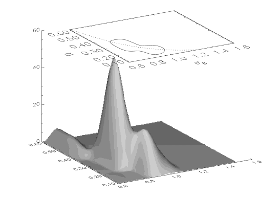
Figure 6: Marginalized probability in $\sigma_{8}-\Omega_{m}$ for the flat $\Lambda$CDM case (for OCDM the situation is similar). The probability distribution has been interpolated in order to smooth the surface. The contour shows the region at the $65$% confidence level and the dotted curve corresponds to the correlation law: $\sigma_{8}=0.5\Omega_{m}^{-0.4}$.

6 Conclusions

In this work, we have shown that our method, which combines different data sets for the cluster population, is a powerful tool to constrain both, the cosmology and cluster scaling relations.
Our method is robust in the sense that neither assumptions about the cosmology nor specific cluster scaling relations are made a priori.
Despite the correlations in the theoretical curves, we have shown that with simple estimators (like the standard $\chi^{2}_{joint}$ and the Lahav et al.’s Bayesian estimator) it is possible to fit the data without any significant bias.

The main conclusions of this paper are the following. Regarding the cosmology we have shown that only low-density (flat and open) models are compatible with the data sets considered in this paper. The marginalized probability in the ($\sigma_{8}-\Omega_{m}$) space shows a clear peak at the position ($\sigma_{8}=0.8$, $\Omega_{m}=0.3$) in both $\Lambda$CDM and OCDM models. This is a very interesting conclusion because previous works (Eke et al. 1996; Kitayama & Suto 1997; Bahcall & Fan 1998; Borgani et al. 1999; Bridle et al. 1999) show a degeneracy in these two parameters. This degeneracy is broken when considering the five data sets we used in this paper. It is important to remark that in Bridle et al. (1999) the authors combine cluster abundance, CMB and IRAS data and they find values for ($\sigma_{8},\Omega_{m}$) very close to our best-fitting model. It is important to note that this result is compatible with the recent determination of the $\Omega_{m}$ parameter obtained by the BOOMERANG team (De Bernardis et al. 2000; Lange et al. 2000) and MAXIMA (Hanany et al. 2000; Balbi et al. 2000).

The third cosmological parameter, $\Gamma$, is consistent with the value obtained from the fit of the power spectrum of galaxies assuming CDM. (Peacock & Dodds 1994, Viana  Liddle 1996)

Regarding the parameters obtained for the cluster scaling relations, they are consistent with empirical determinations of such scalings. However, we find a tendency to high values in the $\alpha$ exponent which could contradict recent determinations of such exponent, Nevalainen et al. (2000). However, as mentioned in the discussion, we know that there is a bias in our estimation of $\alpha$. Therefore our estimate is compatible (within the error bars and the bias) with the virial exponent $\alpha=2/3$.
Additional data coming from high redshift clusters (CHANDRA, XMM-Newton, PLANCK) will improve this result.
Particularly interesting is the work that can be done with future CMB surveys. The PLANCK satellite will explore the whole sky at different frequencies (from 30 Ghz to 800 Ghz) and with resolutions between 5 arcmin and 30 arcmin. At these frequencies and with those resolutions we have shown (Diego et al. 2000) that many clusters are expected to be observed at high redshift ($z>2$) through the Sunyaev-Zel’dovich effect (see fig. 7). PLANCK is expected to detect those clusters with $S_{mm}>30$ mJy. The information these clusters will provide will be decisive to definitely exclude many models. As shown for instance in Barbosa et al. (1996), Aghanim et al. (1997), Diego et al. (2000), the SZE can be considered as a clear probe of the cosmological parameters. In particular, from the previous discussion we concluded that we are not able to discriminate between $\Lambda$CDM and OCDM models. However, from fig. 7, it is evident that through the SZE it could be possible to distinguish between these two models at a very high confidence level.

Figure 7: Prediction of the integrated number counts of cluster population al mm wavelengths (353 GHz) (SZE) for the best flat (solid) and open (dotted) models in table 1. In the plot three redshift shells are represented: top $z<1$, middle $z\in[1,2]$ and bottom $z>2$.

7 Acknowledgments

We would like to thank to Piero Rosati for kindly providing his data for the differential flux function and Nabila Aghanim for useful comments. This work has been supported by the Comisioón Conjunta Hispano-Norteamericana de Cooperación Científica y Tecnológica ref. 98138, Spanish DGESIC Project no. PB98-0531-C02-01, FEDER Project, no. 1FD97-1769-C04-01 and the EEC project INTAS-OPEN-97-1992.
JMD acknowledges support from a Spanish MEC fellowship FP96-20194004. And finally JMD, EMG, JLS, and LK thank to the CfPA and Berkeley Astronomy Dept. for its hospitality during several stays in 1999.

References

- [1] Aghanim N., de Luca A., Bouchet F. R., Gispert R., Puget J. L., 1997, A & A, 325, 9.
- [2] Arnaud M., Evrard A., 1999, MNRAS, 305, 631.
- [3] Bahcall N.A., Cen R. 1993, ApJ, 407, L49.
- [4] Bahcall N.A., Fan X., 1998, ApJ, 504, 1.
- [5] Balbi A. et al. 2000. Preprint astro-ph/0005124
- [6] Barbosa D., Bartlett J., G., Blanchard A., Oukbir J., 1996, A&A, 314, 13.
- [7] Bardeen J.M., Bond J.R., Kaiser N., Szalay A.S., 1986, ApJ, 304, 15.
- [8] Bennet C. L. et al. 1996, ApJ, 464, L1
- [9] Biviano A., Girardi M., Giuricin G., Mardirossian F., Mezzetti M., 1993, ApJ, 411, L13.
- [10] Blanchard A., Sadat R., Bartlett J.G., Le Dour M., 2000, A & A, 362, 809.
- [11] Borgani S., Rosati P., Tozzi P., Norman C., 1999, ApJ, 517, 40.
- [12] Bridle S.L., Eke V.R., Lahav O., Lasenby A.N., Hobson M.P., Cole S., Frenk C.S., Henry J.P., 1999, MNRAS, 310, 565.
- [13] Burke D.J., Collins C.A., Sharples R.M., Romer A.K., Holden B.P., Nichol R.C., 1997, ApJ, 488, L83.
- [14] Carlberg R.G., Morris, S.L., Yee H.K.C., Ellingson E., 1997, ApJ, 479, L19.
- [15] David L.P., Slyz C.J., Forman W., Vrtilek, Arnaud K.A., 1993, ApJ, 412, 479.
- [16] De Bernardis P., et al. 2000, Nature, 404, 955.
- [17] Diego J.M., Martínez-González E., Sanz J.L. Benitez N., Silk J., 2001, MNRAS submitted.
- [18] Donahue M., 1996, 468, 79.
- [19] Donahue M., Voit G.M., 1999, ApJ, 523, L137.
- [20] De Grandi S., et al., 1999, ApJ, 514, 148.
- [21] Ebeling H., Wiedenmann G., 1993, Physical Review E, 47, 704.
- [22] Ebeling H., Edge A.C., Fabian A.C., Allen S.W., Crawford C.S., 1997, ApJ, 479, L101.
- [23] Ebeling H., Edge A.C., Böhringer H., Allen S.W., Crawford C.S., Fabian A.C., Voges W., Huchra J.P., 1998, MNRAS, 301, 881.
- [24] Efstathiou G., Frenk C.S., White S.D.M., Davis M., 1988, MNRAS, 235, 715.
- [25] Eke V.R., Cole S., Frenk C.S., 1996, MNRAS, 282, 263.
- [26] Eke V.R., Cole S., Frenk C.S., Henry, J.P. 1998, MNRAS, 298, 114.
- [27] Evrard A.E., Metzler C.A., Navarro J.F., 1996, ApJ, 469, 494.
- [28] Fairley B.W., Jones L.R, Scharf C., Ebeling H., Perlman E., Horner D., Wegner G., Malkan M., accepted for publication in MNRAS, preprint astro-ph/0003324.
- [29] Fabian A.C., Crawford C.S., Edge A.C., Mushotzky R.F., 1994, MNRAS, 267, 779.
- [30] Girardi M., Borgani S., Giuricin G., Mardirossian F., Mezzetti M., 1998, ApJ, 506, 45.
- [31] Hanany S., et al. 2000. Preprint astro-ph/0005123.
- [32] Henry J.P., Arnaud K.A., 1991, ApJ, 372, 410.
- [33] Henry J.P., 1997, ApJ, 489, L1.
- [34] Henry J.P. 2000, ApJ, 534, 565.
- [35] Horner D.J, Mushotzky R.F, Scharf C.A., 1999, ApJ, 520, 78.
- [36] Kitayama T., Suto Y., 1996, ApJ, 469, 480.
- [37] Kitayama T., Suto Y., 1997, ApJ, 490, 557.
- [38] Lacey C., Cole S., 1994, MNRAS, 271, 676.
- [39] Lahav O., Edge A.C., Fabian A.C., Putney A., 1989, MNRAS, 238, 881.
- [40] Lahav O., Bridle S.L., Hobson M.P., Lasenby A.N., Sodr’e L.Jr., 1999 astro-ph/9912105.
- [41] Lange A.E., et al. 2000, preprint astro-ph/0005004.
- [42] Lupino G.A., Gioia I.M., 1995, ApJ, 445, L77.
- [43] Markevitch M., 1998, ApJ, 504, 27.
- [44] Mathiesen B., Evrard A.E., 1998, MNRAS, 295, 769.
- [45] Mushotzky R.F., Scharf C.A., 1997, ApJ, 482, L13.
- [46] Neumann D. M., Arnaud M., 1999, A&A, 348, 711.
- [47] Nevalainen J., Markevitch M., Forman W., 2000, ApJ, 532, 694.
- [48] Oukbir J., Blanchard A., 1992, A&A, 262, L21.
- [49] Oukbir J., Blanchard A., 1997, A&A, 317, 1.
- [50] Page M.J., Carrera F.J., 2000, MNRAS, 311, 433.
- [51] Peacock J.A., Dodds S.J., 1994, MNRAS, 267, 1020.
- [52] Peebles J., ’The Large-Scale Structure of the Universe’, Princeton Series in Physics, 1980
- [53] Piccinotti G., Mushotzky R.F., Boldt E.A., Holt S.S., Marshall F.E., Serlemitsos P.J., Shafer R.A., 1982, ApJ, 253, 485.
- [54] Press W.H., Schechter P., 1974, ApJ, 187, 425.
- [55] Reichart D.E., Castander F.J., Nichol R.C., 1999, ApJ, 516, 1.
- [56] Romer et al. 2000, ApJS, 126, 209.
- [57] Rosati P., Della Ceca R., Burg R., Norman C., Giacconi R., 1995, ApJ, 445, L11.
- [58] Rosati P., Della Ceca R., Norman C., Giacconi R., 1998, ApJ, 492, L21.
- [59] Scharf C.A., Jones L.R.L., Ebeling H., Perlman H., Malkam M., Wegner G., 1997, ApJ, 477, 79.
- [60] Viana P.T., Liddle A.R. 1996, MNRAS, 281, 323.
- [61] Vikhlinin A., McNamara B.R., Forman W., Jones C., Quintana H., Hornstrup A., 1998, ApJ, 502, 558.
- [62] Voges et al. 1999, A&A, 349, 389.
- [63] Voit G.M., Donahue M., 1998, ApJ, 500, L111.
- [64] White S.D.M., Efstathiou G., Frenk C.S., 1993, MNRAS, 262, 1023.
- [65] White D.A., Jones C., Forman W., 1997, MNRAS, 292, 419.