Scaling properties of the redshift power spectrum: theoretical models

Abstract

We report the results of an analysis of the redshift power spectrum $P^{S}(k,\mu)$ in three typical Cold Dark Matter (CDM) cosmological models, where $\mu$ is the cosine of the angle between the wave vector and the line–of–sight. Two distinct biased tracers derived from the primordial density peaks of Bardeen et al. and the cluster–underweight model of Jing, Mo, & Börner are considered in addition to the pure dark matter models. Based on a large set of high resolution simulations, we have measured the redshift power spectrum for the three tracers from the linear to the nonlinear regime. We investigate the validity of the relation –guessed from linear theory–in the nonlinear regime

$$P^{S}(k,\mu)=P^{R}(k)[1+\beta\mu^{2}]^{2}D(k,\mu,\sigma_{12}(k))\,,$$ (1)

where $P^{R}(k)$ is the real space power spectrum, and $\beta$ equals $\Omega_{0}^{0.6}/b_{l}$. The damping function $D$ which should generally depend on $k$, $\mu$, and $\sigma_{12}(k)$, is found to be a function of only one variable $k\mu\sigma_{12}(k)$. This scaling behavior extends into the nonlinear regime, while $D$ can be accurately expressed as a Lorentz function– well known from linear theory– for values $D>0.1$. The difference between $\sigma_{12}(k)$ and the pairwise velocity dispersion defined by the 3–D peculiar velocity of the simulations (taking $r=1/k$) is about $15\%$. Therefore $\sigma_{12}(k)$ is a good indicator of the pairwise velocity dispersion. The exact functional form of $D$ depends on the cosmological model and on the bias scheme. We have given an accurate fitting formula for the functional form of $D$ for the models studied.

1 Introduction

In general the redshift of a galaxy gives a reasonable measure of its distance. It is, however, exact only when the galaxy follows the linear Hubble flow, and there are two distinct deviations from that: observations of high redshift objects require an assumption about the cosmic geometry, and choosing, e.g., a wrong cosmological model may create for an intrinsically isotropic spatial distribution of objects anisotropies along the line of sight and along the line projected perpendicularly (Alcock & Paczynski (1979); Matsubara & Suto (1996); Ballinger, Peacock & Heavens (1996)). The peculiar motions of galaxies induced by the gravitational field of clumpy structures also change the true distribution (Geller & Peebles (1973); Turner (1976); Davis & Peebles (1983); Kaiser (1987)). Therefore in redshift space we find a distorted picture of the spatial distribution. This may seem unfortunate, but, on the other hand, it allows to estimate the statistics of the clustering process. A careful modeling of these effects can yield valuable determinations of the cosmological model parameters, the power spectrum, and the bias of these objects.

The statistic widely used for measuring the redshift distortion is the redshift two-point correlation function or equivalently its Fourier counterpart, the redshift power spectrum. In this paper we will focus our discussion on the redshift power spectrum. The models for the cosmological geometry effect on these statistics have been well established (Matsubara & Suto (1996); Ballinger, Peacock & Heavens (1996)), since there exists a simple mathematical mapping of a redshift spatial distribution from one cosmological model to another. More uncertainties however exist in the theoretical modeling of the effects of the peculiar motion. These uncertainties will affect the modeling of the redshift distortion not only at low redshift but also at high redshift, since the peculiar motion is likely to be also important for redshift surveys of quasars and galaxies (e.g. Adelberger, et al. (1998); Steidel et al. (1998)) at high redshift (Suto, et al. (1999); Magira, Jing & Suto (2000)). Therefore it is highly desirable to have an accurate model for the peculiar motion effect.

In the limits of a linear density perturbation and of a linear galaxy bias, the redshift power spectrum $P^{S}_{\rm l}(k,\mu)$ can be accurately derived (Kaiser (1987)),

$$P^{S}_{\rm l}(k,\mu)=P^{R}_{\rm l}(k)[1+\beta\mu^{2}]^{2}\,.$$ (2)

In the above equation, $\mu$ is the cosine of the angle between the wavevector $\bf k$ and the line-of-sight; $P^{R}_{\rm l}$ is the linear power spectrum in real space; $\beta$ equals $\Omega_{0}^{0.6}/b_{l}$, where $b_{l}$ is the linear bias parameter and $\Omega_{0}$ is the density parameter of the universe. Throughout the paper, we will use superscripts $S$ and $R$ to denote quantities in redshift space and in real space respectively. In another extreme limit of collapsed objects (the finger-of-God effect), the redshift distortion was found observationally to be described by an exponential distribution function (DF) for the pairwise velocity (Peebles (1976); Davis & Peebles (1983)), though significant uncertainties must be allowed for these observations. Subsequent theoretical studies based on numerical simulations (Efstathiou, et al. (1988)), the Press & Schechter (1974) theory (Diaferio & Geller (1996); Sheth (1996)) and the Zeldovich approximations (Seto & Yokoyama (1998)) have confirmed that the distribution function of the pairwise velocity can be well approximated by an exponential form for the dark matter in currently favored CDM models and in some scale-free hierarchical clustering models. Based on the assumptions that a) the DF of the pairwise velocity has an exponential form, b) the linear (Kaiser (1987)) and the nonlinear (Finger-of-God) effects are separable, and c) there is only weak coupling between the density and the non-linear motion, it is not difficult to derive an ansatz for the redshift distortion of the power spectrum on all scales (Peacock & Dodds (1994); Cole, Fisher & Weinberg (1995)):

$$P^{S}(k,\mu)=P^{R}(k)[1+\beta\mu^{2}]^{2}{1\over 1+{1\over 2}(k\mu\sigma_{v})^{2}}\,.$$ (3)

This formula has been compared to N-body simulations (Cole, Fisher & Weinberg (1994); Cole, Fisher & Weinberg (1995); Bromley, Warren & Zurek (1997); Magira, Jing & Suto (2000)), and it has turned out that equation (3) describes the redshift power spectrum of dark matter accurately on large scales ($k\mathrel{\raise 1.16pt\hbox{$<$}\kern-7.0pt\lower 3.06pt\hbox{{$\scriptstyle\sim$}}}0.2\,h{\rm{Mpc}}^{-1}$, i.e. in the linear and quasi-linear regime) with $\sigma_{v}$ equal to the pairwise velocity dispersion at large separation (Magira, Jing & Suto (2000)).

Equation (3) can at best be an approximation for describing the redshift power spectrum for several reasons. For the clustering on large scales, the coupling between the non-linear motion and the structures is weak and the DF of the pairwise velocity is described well by the exponential form (at least in many hierarchical clustering models). This might be the reason why equation (3) has been found to be in good agreement with numerical simulations on large enough scales. However, at smaller and smaller scales, the coupling between the non-linear motions and the structures becomes stronger and stronger. It is also probably not a valid procedure to extrapolate the model of linear motion (Kaiser (1987)) to the non-linear regime to model the infall on small scales. Furthermore it has been found in simulations that the DF of the pairwise velocity is significantly skewed in the quasi-linear regime to the approaching velocity of particle pairs (Juszkiewicz, Fisher & Szapudi (1998); Magira, Jing & Suto (2000)). For all these reasons, we may expect that equation (3) breaks down on non-linear scales. Some deviation of this model from simulation data could already be seen in previous studies (Cole, Fisher & Weinberg (1995); Bromley, Warren & Zurek (1997); Magira, Jing & Suto (2000)) even in the quasi-linear regime ($k\mathrel{\raise 1.16pt\hbox{$>$}\kern-7.0pt\lower 3.06pt\hbox{{$\scriptstyle\sim$}}}0.5\,h{\rm{Mpc}}^{-1}$), though the focus of those studies is on the agreement of the equation with the simulation data in the linear regime.

We devote this paper to studying the redshift power spectrum in the non-linear and quasi-linear regimes. With the help of a large set of high resolution simulations, we measure the redshift power spectrum for dark matter from linear to strongly non-linear regimes. We find that while equation (3) starts to break down in the quasi-linear regime, there exists a scaling relation of the variable $k\mu\sigma_{v}$ for the non-linear effects (motion and coupling between density and velocity). The existence of this scaling relation is not trivial, since there is a strong coupling between the velocity and the density on non-linear scales. But such a scaling relation would be very useful for studying and quantifying the redshift power spectrum on small scales in observational catalogs (§4). Since the galaxies in the universe do not generally trace the distribution of the underlying matter, we will also study the redshift power spectrum for two plausible bias models: the primordial peaks (Bardeen, et al. (1986)) and the cluster-under-weight bias (Jing, Mo & Börner (1998); hereafter JMB98). We find that scaling relations of the variable $k\mu\sigma_{v}$ exist in both bias models. The scaling form as a function of the variable $k\mu\sigma_{v}$ depends on the bias model. Therefore a determination of this scaling function from observations may be used to discriminate between different models of galaxy formation.

The paper is arranged as follows: in the next section, we will describe the simulation samples and the bias models used. The techniques for measuring the redshift power spectrum are outlined, and the results are presented in section 3. The final section, §4, is devoted to discussion and conclusions.

2 Simulation sample and simple bias models

We study the redshift distortion of the power spectrum for three Cold Dark Matter (CDM) models, i.e. the standard CDM (SCDM), a flat low-density CDM (LCDM), and an open CDM (OCDM). The model parameters are given in Table 1, with $\Omega_{0}$ for the density parameter, with $\lambda_{0}$ for the cosmological constant, and with $\Gamma=\Omega_{0}h$ and $\sigma_{8}$ respectively for the shape parameter and the normalization of the linear power spectrum. These models constitute a typical set of CDM models. Our N-body simulations are those of Jing & Suto (1998) and Jing (1998), with box sizes of $100\,h^{-1}{\rm{Mpc}}$ and $300\,h^{-1}{\rm{Mpc}}$. Each model has three to four statistical realizations for one box size. All the simulations employ $256^{3}$ ($\approx 17$ million) particles and were generated with our $\rm P^{3}M$ code on the Fujitsu vector machines at the National Astronomical Observatory of Japan. The simulations have been used for studying a number of cosmological problems. A summary of these applications and the simulation details can be found in Jing (2000).

While we can extract valuable information on the dark matter distribution from N-body simulations, galaxies observed in the Universe most likely do not exactly trace the underlying dark matter distribution. The so-called “bias” of the galaxy distribution with respect to the underlying matter distribution remains one of the unsolved outstanding problems in cosmology. To study the effect of the bias on the redshift distortion, we take two simple bias models: the primordial peak model of Bardeen et al. (1986) and the cluster-under-weighted (CLW) model of JMB98. Because of the long-wavelength modulation of the primordial density perturbation, the peak model ascribes more weight to the high density (cluster) regions in the spatial distribution than the pure dark matter model, while the CLW model, by its construction, gives less weight to the cluster regions than the dark matter model. The redshift distortion in the non-linear regime is known to be sensitive to the weighting of the cluster regions. These bias models cover many facets of the bias effect on the redshift distortion.

In our peak model, peaks are defined as fluctuations with more than 2 times the rms fluctuation of the primordial density field smoothed with a Gaussian window $\exp(-r^{2}/2r_{s}^{2})$. The window width is taken to be $r_{s}=0.54\,h^{-1}{\rm{Mpc}}$ so that the peaks are relevant for galactic-sized objects. We follow the prescription of White, et al. (1987) to assign an expectation number of peaks to each simulation particle in Lagrangian space (see Jing, et al. (1994) for a detailed description of our algorithm). During the dynamical evolution, these peaks stay with the particles to which they are assigned. Because our simulations have a high mass resolution, the expectation number of peaks per particle is always less than 1.

Our cluster weighting bias model is the same as that of JMB98. Specifically, the number of galaxies per unit dark matter mass $N/M$ is proportional to $M^{-0.08}$ within a massive halo of mass $M$, i.e. the cluster regions are under-weighted. We identify clusters in the N-body simulations using the friends-of-friends method with a linkage parameter equal to 0.2 times the mean separation of particles. We randomly throw away particles in clusters according to the above bias model. Typically 10 percent of the total number of simulation particles, mostly in cluster regions, have been left out. This phenomenological model was proposed by JMB98 to reconcile the CDM models with their measurement for the two-point correlation function and the pairwise velocity dispersion in the Las Campanas Redshift Survey. This empirical model has also received support from the observation of the CNOC clusters (Carlberg, et al. (1996)) where a similar trend of $N/M$ has shown up, though the scatter in the observation is still large. There is evidence that this empirical model is also consistent with semi-analytical models of galaxy formation which incorporate star formation (Benson, et al. (1999)), since these semi-analytical models have produced predictions for the two-point correlation function and the velocity dispersion quite similar to the empirical model.

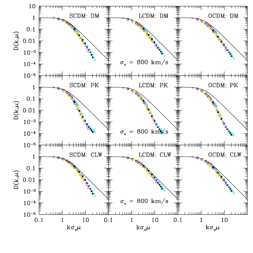
Figure 4: The damping function $D(k,\mu)$ determined according to Equation (4) is plotted as a function of $k\mu\sigma_{v}$ with $\sigma_{v}$ fixed to $800\,{\rm{km\,s^{-1}}}$. The curves are the prediction of the Lorentz form. The symbols and the labels are the same as in Fig. 2

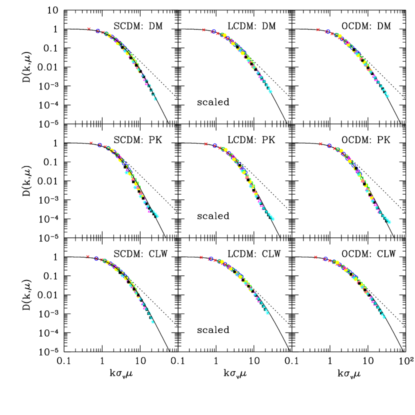
Figure 5: The same as Fig. 4, but the velocity dispersion $\sigma_{v}$ is allowed to vary with the wavenumber $k$. The dashed curves are the prediction of the Lorentz form and the solid ones are given by the fitting formula Eq.(5) with the $\eta$ given in Table 2. The values of $\sigma_{v}(k)$ used for this plot are given in Fig. 6.

The bias factors $b(k)$ of these biased models, which are measured from the square root of the ratio of the real space power spectrum of the biased tracer to that of the underlying dark matter, are presented in Figure 1. The bias function is a constant $b_{l}$ on large scales ($k<0.08\,h{\rm{Mpc}}^{-1}$). It rises on small scales in the peak models, but slightly falls with $k$ in the cluster-weight models (though it does not rise or fall monotonically at the smallest scales). The effects of the non-linear bias functions on the linear Kaiser effect are examined by looking at the ratio $[1+\mu^{2}\Omega_{0}^{0.6}/b(k)]^{2}/[1+\mu^{2}\Omega_{0}^{0.6}/b_{l}]^{2}$. For each $k$, the ratio reaches the maximum deviation from $1$ at $\mu=1$. Figure 2 shows that replacing $b(k)$ with $b_{l}$ in modeling the linear Kaiser effect could result in an error of $\mathrel{\raise 1.16pt\hbox{$<$}\kern-7.0pt\lower 3.06pt\hbox{{$\scriptstyle\sim$}}}20\%$ in the damping factor (§3) in the non-linear regime. Since the linear bias can be analytically calculated for the bias models (e.g. Matsubara (1999)) and an error of $\sim 20\%$ in $D$ is tolerable in this study (cf. Fig. 4 and Fig. 5), we will use the linear bias factor to model the linear Kaiser effect throughout this paper.

3 Redshift power spectrum

3.1 Measurement method

We choose the third axis as the line-of-sight direction, and map the coordinate positions of the simulation particles from real space to redshift space by taking into account each particle’s peculiar velocity. Periodic boundary conditions are used to place back into the simulation box those particles which are outside of the box in redshift space. A grid of $640^{3}$ uniformly spaced points is placed within the simulation box. The Nearest-Grid-Point (NGP) method is used to get the density of dark matter or peaks on the grid. This grid of density is transformed to the density distribution in Fourier space $\delta({\bf k})$ using the Fast Fourier Transform (FFT) method. The Nyquist wavenumber $k_{N}$ is about $6.7\,h{\rm{Mpc}}^{-1}$ for a box size of $300\,h^{-1}{\rm{Mpc}}$ and $20\,h{\rm{Mpc}}^{-1}$ for a box size of $100\,h^{-1}{\rm{Mpc}}$. We take linear bins for $\mu$ with $\Delta\mu=0.1$, with an additional bin at $\mu=0$. For the wavenumber $k$, equal logarithmic bins $\Delta\lg(k)=0.1$ are taken from $0.05k_{N}$ to $k_{N}/4$. The lower limit for $k$ is chosen such that there are sufficient modes and the sample-to-sample fluctuation in $\delta({\bf k})$ is small. The upper limit is taken such that the biases introduced by the FFT method are negligible.

The assignment of mass and peaks to a grid for FFT brings about artificial smearing as well as artificial anisotropy to the density field $\delta({\bf k})$ near the Nyquist wavenumber. These artificial effects on the power spectrum measurement have been discussed in detail by Jing (1992). Although these effects might be corrected with an iterative procedure(cf Jing 2000), we adopt a simpler approach here. We limit our discussion to small wavenumbers, where these effects become negligible. Indeed, for the NGP assignment scheme adopted here, these effects are seen to diminish for wavenumbers $k\leq k_{N}/4$, according to Jing (1992, 2000). To show this point quantitatively, we measure the redshift power spectrum for one LCDM simulation of box size $100\,h^{-1}{\rm{Mpc}}$ with $320^{3}$ and $640^{3}$ grid points respectively. The ratio of these redshift power spectra at $k=2.3\,h{\rm{Mpc}}^{-1}$, about one fourth of the Nyquist wavenumber for the grid points of $320^{3}$, is 0.98 and nearly independent of $\mu$. Thus the redshift power spectrum is underestimated by only 2 percent in the case of $320^{3}$. This accuracy is good enough for this study. In the following, our results will be presented for $k\leq k_{N}/4$.

3.2 Results

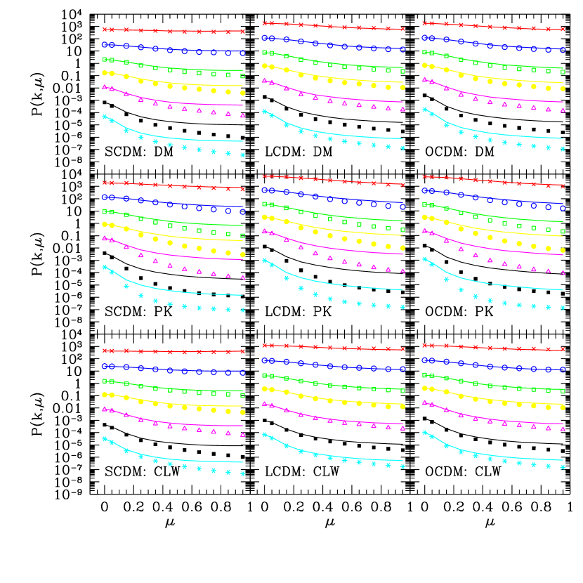
Figure 3: The redshift power spectrum $P^{S}(k,\mu)$ determined for the different tracers of the three CDM models. The top panels are for the dark matter (DM), the middle for the peaks (PK), and the bottom for the cluster under weighted population (CLW). In each panel, $P^{S}(k,\mu)$ at different $k$ are plotted with different symbols. From the top (crosses) to the bottom (stars), the values of $k$ are 0.35, 0.56, 0.90, 1.1, 1.7, 2.7, 3.4 $\,h^{-1}{\rm{Mpc}}$ respectively, and the $P^{S}(k,\mu)$ are multiplied by $1$, $10^{-1}$, $10^{-2}$, …, $10^{-6}$ respectively for clarity. The lines are the model prediction of Equation (3) where the Lorentz form is used for the damping function.

The redshift power spectrum $P^{S}(k,\mu)$ which we have measured for the dark matter is presented in the top panels of Figure 3. Different symbols are used for $P^{S}(k,\mu)$ at different $k$, with $k$ increasing from the symbols at the top to those at the bottom. The smallest and the largest values of $k$ are $0.35\,h{\rm{Mpc}}^{-1}$ and $3.4\,h{\rm{Mpc}}^{-1}$ respectively, and the increment of $k$ between two successive sets of symbols is $\Delta\log_{10}k=0.2$ approximately. Thus we obtain a sequence for the redshift power spectrum from the quasi-linear to the highly non-linear regimes. The non-linear peculiar motion suppresses the clustering along the line-of-sight, with the effect manifested more prominently at larger $k$ and larger $\mu$. The power spectrum is suppressed by 3 magnitudes along the line-of-sight at the largest $k$ values, indicating that we have approached the highly non-linear regime. In all three dark matter models, we find these same qualitative features for $P^{S}(k,\mu)$ .

The curves for each $k$, which always start from the data points at $\mu=0$, are the model prediction of Equation (3) with $\beta=\Omega_{0}^{0.6}$ for each simulation. For $\sigma_{v}(k)$, we have used the pairwise velocity dispersion at the separation $r=1/k$ . The model agrees well with the simulation data for large scales $k\mathrel{\raise 1.16pt\hbox{$<$}\kern-7.0pt\lower 3.06pt\hbox{{$\scriptstyle\sim$}}}0.5\,h{\rm{Mpc}}^{-1}$. But at large $k$ where the non-linearity is strong, the model predicts a significantly slower decrease with $\mu$ than the simulation data. Adjusting the value for $\sigma_{v}(k)$ could not produce a better match between the model and the simulation data.

The redshift power spectra for the peaks and the cluster-weighted particles are shown in the middle and bottom panels of Figure 3 respectively. The qualitative features of these biased models are very similar to those of the dark matter. But with a closer look at the figures, we can easily find that among the three models, the peak model has the strongest dependence on $\mu$ and the cluster weighted model has the weakest. The results are expected, since the cluster regions are over– weighted in the peak model and under– weighted in the CLW model relative to the pure dark matter model. When calculating predictions for these biased models, we use the bias parameter $b_{l}$ determined on the linear scale. The simulation results of the biased models, like those of the pure dark matter models, show a faster decrease with $\mu$ for high $k$, indicating that equation (3) is not adequate for describing the redshift distortion in the highly non-linear regime even if we let $\sigma_{v}$ be a function of $k$.

It is not unexpected that equation (3) breaks down in the non-linear regime for the reasons outlined in Section 1. In order to study the non-linear behavior of the redshift power spectrum, we examine the relation

$$D(k,\mu)\equiv{P^{S}(k,\mu)\over P^{R}(k)(1+\beta\mu^{2})^{2}}\,,$$ (4)

where we take the damping function now to be an unknown quantity $D(k,\mu)$ which should be determined from the known expressions on the right hand side. The factor $(1+\beta\mu^{2})^{2}$ accounts for the linear distortion of the power spectrum. The power spectrum $P^{R}(k)$ in real space is measured as in Jing (2000). This will be used for the denominator of equation (4). In equation(3), the damping function has the Lorentz form ,i.e. it is a function of $k\mu\sigma_{v}$ only. Despite the fact that the Lorentz form is inadequate in the non-linear regime, we find that the damping function is approximately a function of $k\mu\sigma_{v}$. We take $800\,{\rm{km\,s^{-1}}}$ for the value of $\sigma_{v}$ which is close to the simulation value. The results are plotted in Figure 4 for the CDM and different bias models, with different symbols for different wavenumbers $k$ (as in Figure 3). The points for different values of $k$ fall on top of each other, and this demonstrates that the damping function is indeed approximately a function of $k\mu\sigma_{v}$. Furthermore the damping function in all the different models falls more steeply than the Lorentz form when $D(k,\mu)<0.1$, which is consistent with Figure 3.

Although the damping function at different $k$ and $\mu$ is approximately a scaling function of $k\mu\sigma_{v}$, there exist small but significant systematic scatters of $D(k,\mu)$ for different $k$ along the horizontal axis $k\mu\sigma_{v}$. The shifts amount typically to a few tens percent in $k\mu\sigma_{v}$. The reason could be that the velocity dispersion is not a constant. In fact, it is well known that the pairwise velocity dispersion in coordinate space is a function of the pairwise separation $r$ and in the CDM models the pairwise velocity dispersion peaks at $r\approx 2\,h^{-1}{\rm{Mpc}}$ (e.g. JMB98). Therefore, we relax the assumption of $\sigma_{v}={\rm constant}$ and let $\sigma_{v}$ vary with $k$.

Figure 5 shows the damping function in the different models as a function of $k\mu\sigma_{v}$, where $\sigma_{v}$ is allowed to vary with $k$. We have taken values for $\sigma_{v}(k)$ such that the damping function $D(k\mu\sigma_{v})$ of two neighboring $k$ bins matches best. This determines the relative values of $\sigma_{v}(k)$. In order to fix the absolute values, we fit the damping function with the Lorentz form for $D(k,\mu)>0.1$. The Lorentz form for $D(k,\mu)>0.1$ describes well the simulation data of all the models (see more discussion below). The values of $\sigma_{v}(k)$ determined in this way are plotted in Figure 6.

The damping function $D(k,\mu)$, plotted as a function of $k\mu\sigma_{v}$, has a much smaller scatter with a variable $\sigma_{v}$ than with a constant one. Although it is not surprising that taking a variable $\sigma_{v}(k)$ improves the scaling relation of $D(k,\mu)$ (since it gives more freedom than a constant $\sigma_{v}$), it is far from trivial to have such a good scaling relation with a variable $\sigma_{v}(k)$, since $k\mu\sigma_{v}$ can vary by an order of magnitude even for a single $k$ and we do not adjust $D(k,\mu)$.

Moreover, the qualitative behavior of $\sigma_{v}(k)$ is very similar to that of the pairwise velocity dispersion (PVD) $\sigma_{PVD}(r)$ which is measured directly from the 3-dimensional peculiar velocity in the simulation. $\sigma_{v}(k)$ peaks at $k\approx 1\,h^{-1}{\rm{Mpc}}$ and gently falls when $k$ increases or decreases. This compares well with the pairwise velocity dispersion $\sigma_{PVD}(r)$ (curves in Figure 6), where we have arbitrarily assumed $k=1/r$ for the horizontal axis. In fact, we can use $\sigma_{PVD}$ from the simulation data for the variable $\sigma(k)$ and obtain damping functions very similar to the graphs shown in Figure 5. Small differences between the use of $\sigma_{PVD}(r)$ and of $\sigma_{v}(k)$ are expected, since there is no reason that they should be exactly the same. But the fact that the difference between $\sigma_{PVD}(r)$ and $\sigma_{v}(k)$ is less than 20% (if $k\propto 1/r$ is used) is very encouraging: $\sigma_{v}(k)$ is a good indicator of the pairwise velocity dispersion $\sigma_{PVD}(r)$, and can be measured in a redshift catalog (see Section 4).

We have fitted the scaled damping function of our simulation with the following form

$$D(k,\mu)={1\over 1+{1\over 2}(k\mu\sigma_{v}(k))^{2}+\eta(k\mu\sigma_{v}(k))^{4}}\,.$$ (5)

The fitting values for the parameter $\eta$ are given in Table 2 for each model. The above fitting formula describes our simulation results very well, as shown by Figure 5. The formula can also be used to compare the theoretical models with the statistic in future large redshift surveys of galaxies.

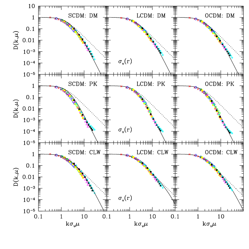
Figure 7: The same as Fig. 5, but the velocity dispersion $\sigma_{v}(k)$ is taken from the pairwise velocity dispersion $\sigma_{PVD}(r)$ at $r=1/k$. The dashed curves are the prediction of the Lorentz form and the solid ones are given by the fitting formula Eq.(5) with the $\eta$ given in Table 3.

It is quite useful to present a simple method for predicting $P^{S}(k,\mu)$ in the theoretical models. One way is to combine Eq.(5) and Fig. 6. One could interpolate the data points in Fig. 6 to get $\sigma_{v}(k)$ and use Eq.(5) to predict the damping function for the models. An alternative way is to replace $\sigma_{v}(k)$ with the PVD of the dark matter $\sigma^{dm}_{PVD}(1/k)$, since the dark matter PVD can be predicted with the fitting formula given by Mo, Jing & Börner (1997). Figure 7 shows the damping function when $\sigma^{dm}_{PVD}(1/k)$ is used for $\sigma_{v}(k)$. The scatters in this figure are slightly larger than those in Figure 5 as expected, but the scaling relation of $D(k,\mu)$ still reasonably holds. The damping function could still be described by the fitting formula (5) with the fitting values of $\eta$ listed in Table 3. One can use these results to predict the redshift power spectrum $P^{S}(k,\mu)$.

We note that the fitting formula of this paper is valid only for the models studied here. It is however possible to work out an analytical model for the redshift power spectrum which is generally applicable to CDM models and to the peak and cluster-weight bias schemes, based on the known physical properties of dark matter halos (cf. Mo, Jing & Börner 1997; Ma & Fry (2000); Mo, Jing & White (1997)). We will study such an analytical model in a subsequent paper.

4 Discussion and Conclusion

As we have shown, there exist good scaling relations for the damping function $D(k,\mu)$ when the scaling variable $k\mu\sigma_{v}(k)$ is used. The conclusion is valid for all the galaxy formation models examined in the paper (i.e. 3 CDM models and 2 bias models), although the scaling form depends both on the dark matter models and the bias models. $D(k\mu\sigma_{v}(k))$ falls with $k\mu\sigma_{v}(k)$ slightly faster in the SCDM model than in the two low-density models. It also falls faster in the cluster-over-weighted models (Peak models) than in the CLW models. For all the models, the damping function $D(k,\mu)$ is approximately described by the Lorentz form for large scales where $D>0.1$, but the simulation result is below the analytical form for smaller scales. The detailed form of the scaling relation is expected to reflect the distribution function of the pairwise velocity as well as the coupling between the velocity and density. Thus it depends on the details of the galaxy formation model and the bias model. We have presented an accurate fitting formula for the damping functions for the models studied.

Our results have several important implications for observation. Because the models studied cover a wide range of parameters, we conjecture that a scaling relation of $D(k,\mu)$ also holds for the galaxies in our Universe. This scaling relation can be measured by the method used in this paper, by analyzing the redshift power spectrum for a redshift catalog of galaxies. The resulting velocity dispersion, though slightly different from the PVD defined by the 3-D peculiar velocity, is a good indicator for it. The fact that both the scaling form of $D(k\mu\sigma_{v}(k))$ and the velocity dispersion depend on the dark matter model as well as on the bias model implies that these quantities can become effective observational tests for theoretical models. The determination for the scaling relation is also important for determining the $\beta$ value when the redshift power spectrum can be precisely measured only up to the scale $2\pi/k\approx 60\,h^{-1}{\rm{Mpc}}$. On this scale or smaller, the nonlinear motion still has appreciable effects and can be corrected by scaling the damping function.

In the traditional analysis of the two-point redshift correlation function (TPRCF, Davis & Peebles (1983)), a functional form must first be assumed for the DF of the pairwise velocity. The validity of the functional form is checked by matching the model TPRCF, which is a convolution of the the real-space two-point correlation with the DF of the pairwise velocity, with the observational data. This method has been applied to various redshift surveys ( Mo, Jing & Börner (1993); Marzke, et al. (1995); Fisher, et al. (1994); Ratcliffe et al. (1998); Postman et al. (1998); Grogin & Geller (1999); Small, et al. (1999)). However, searching for the functional form of the DF of the pairwise velocity in parameter space is much more difficult than determining its Fourier counterpart, the damping function, from an analysis of the redshift power spectrum. Moreover, in modeling the TPRCF, an infall velocity as a function of $r$ must be assumed (Davis & Peebles (1983)). The functional form of the infall velocity is less well understood (Marzke, et al. (1995); Jing & Börner (1998)) and much more difficult to determine in observations than the the single parameter $\beta$ in the power spectrum analysis. The velocity dispersions measured in both analyses are shown to have similar accuracy (difference $\mathrel{\raise 1.16pt\hbox{$<$}\kern-7.0pt\lower 3.06pt\hbox{{$\scriptstyle\sim$}}}20\%$) compared to the 3-D peculiar velocity dispersion (e.g. JMB98; Jing & Börner (1998)). Through this comparison, it is clear that the two types of the redshift clustering analysis complement each other, but an analysis of the redshift power spectrum has the above mentioned advantages over the analysis of TPRCF.

In previous studies of the redshift power spectrum in CDM models (e.g. Cole, Fisher & Weinberg (1994), 1995; Magira, Jing & Suto (2000); Bromley, Warren & Zurek (1997); Fisher & Nusser (1996); Taylor and Hamilton (1996); Hatton & Cole (1999)), the authors studied the behavior of $P^{S}(k,\mu)$ mainly in the quasi-linear regime, with emphasis on the agreement of Equation (3) with the simulation data. Their results were presented usually for the monopole and quadrupole of $P^{S}(k,\mu)$ only, instead of the full dependence on $\mu$ as in this paper. With the exception of Bromley et al. (1997) who considered dark matter halos, most previous work was concerned with the redshift power spectrum for the dark matter only. In comparison, our present work has focused on the full dependence of $P^{S}(k,\mu)$ on $\mu$ from the quasilinear to the highly non-linear regime. To achieve this goal, we have used a large set of high-resolution N-body simulations. We have also paid close attention to the artificial biases introduced by the FFT method, and we have included two distinctive bias models in order to study the dependence of $P^{S}(k,\mu)$ on the galaxy bias. Moreover, we have given an accurate fitting formula for $P^{S}(k,\mu)$ for all the models studied here. Thus we present here a very thorough study of the redshift power spectrum.

In summary, we have carried out a very systematic, detailed analysis for the redshift distortion of the power spectrum in currently popular models of galaxy formation, paying special attention to the strongly non-linear regime. Three CDM models and two distinct bias models for each CDM model are considered, with a total of nine models. A large set of high-resolution simulations of $256^{3}$ particles are used to trace the linear and nonlinear clustering in these models. We have carefully checked the FFT method and avoided those systematic biases inherent to the method on small scale (or large $k$). Our main results are:

1. The redshift power spectrum $P^{S}(k,\mu)$ can be accurately expressed by Equation (1) with the damping function $D(k,\mu)$ being a scaling function of the variable $k\mu\sigma_{v}(k)$ in all the models studied here. An accurate fitting formula has been given for these scaling functions.

2. A mild variation of $\sigma_{v}(k)$ with the scale $k$ is required to improve the scaling relation of $D(k,\mu)$ among different scales. The behavior of $\sigma_{v}(k)$ with the scale is qualitatively similar to that seen in the PVD defined by the 3D peculiar velocity. Therefore, the variation of $\sigma_{v}(k)$ with the scale in fact reflects the separation dependence of the PVD, although there is about $20\%$ systematic difference between these two quantities.

3. The damping function is described well by the Lorentz form for $D(k\mu\sigma_{v})>0.1$ but falls faster than the Lorentz form on smaller scales ($D(k\mu\sigma_{v})<0.1$). The most likely cause for the deviation is the strong coupling between the nonlinear motion and the small scale structures.

4. The functional form of $D(k\mu\sigma_{v})$ as well as the quantity $\sigma_{v}(k)$ depends on the dark matter models and the bias recipes. An observational measurement of these two quantities can serve as an interesting test for models of galaxy formation.

Because of these interesting features of $P^{S}(k,\mu)$, an observational analysis of the redshift power spectrum, though it is largely complementary to, has several obvious advantages over the traditional analysis of the two-point correlation function. In a subsequent paper, we (Jing & Börner (2000)) will apply the results of this paper to measure the damping function and the velocity dispersion for the currently largest redshift survey- the Las Campanas Redshift Survey (Shectman et al. (1996)).

All the data presented in the figures are available to the interested readers in electronic form upon request.

Table 1.   Model parameters

Model	$\Omega_{0}$	$\lambda_{0}$	$\Gamma$	$\sigma_{8}$
SCDM	1.0	0.0	0.5	0.6
OCDM	0.3	0.0	0.25	1.0
LCDM	0.3	0.7	0.21	1.0

Table 2.   The fitting values of $\eta$

	DM	Peaks	CLW
SCDM	0.00965	0.0204	0.00792
OCDM	0.00330	0.0168	0.00171
LCDM	0.00309	0.0168	0.00145

Table 3.   The fitting values of $\eta$ when $\sigma_{v}(k)$ is replaced with $\sigma_{PVD}(1/k)$

	DM	Peaks	CLW
SCDM	0.01118	0.0401	0.00327
LCDM	0.00759	0.0481	0.00089
OCDM	0.00566	0.0429	0.00021

Figure 1: The bias factor $b(k)$ measured as the square root of the ratio of the power spectrum of the biased tracer to that of the dark matter.

Figure 2: The ratio of $[1+\Omega_{0}^{0.6}/b(k)]^{2}$ to $[1+\Omega_{0}^{0.6}/b_{l}]^{2}$, where $b_{l}$ is the bias on the linear scale. The curves represent the maximum effect that the non-linear bias has on the linear Kaiser effect at $\mu=1$.

Figure 6: The velocity dispersion $\sigma_{v}(k)$ (symbols) required to make the damping function a scaling function of $k\mu\sigma_{v}$, compared to the pairwise velocity dispersions measured from the true peculiar velocity(curves). The open symbols and the dotted lines are for the simulations of $300\,h^{-1}{\rm{Mpc}}$, and the solid symbols and the solid lines for those of $100\,h^{-1}{\rm{Mpc}}$. The systematic difference of the velocity dispersion at $k\sim 1\,h{\rm{Mpc}}^{-1}$ between the two box sizes, which is small (5% only), is due to the different long wavelength cutoff in the simulation.

References

- Adelberger, et al. (1998) Adelberger, K. L., Steidel, C. C., Giavalisco, M. , Dickinson, M. , Pettini, M. & Kellogg, M. 1998, ApJ, 505, 18
- Alcock & Paczynski (1979) Alcock, C. & Paczynski, B. 1979, Nature, 281, 358
- Ballinger, Peacock & Heavens (1996) Ballinger, W. E., Peacock, J. A. & Heavens, A. F. 1996, MNRAS, 282,877
- Bardeen, et al. (1986) Bardeen, J. M., Bond, J. R., Kaiser, N. & Szalay, A. S. 1986, ApJ, 304, 15
- Benson, et al. (1999) Benson, A. J., Baugh, C. M., Cole, S., Frenk, C. S., & Lacey, C. G. 1999, astro-ph/9911179
- Bromley, Warren & Zurek (1997) Bromley, B. C., Warren, M. S. & Zurek, W. H. 1997, ApJ, 475, 414
- Carlberg, et al. (1996) Carlberg, R. G., Yee, H. K. C., Ellingson, E., Abraham, R., Gravel, P., Morris, S. & Pritchet, C. J. 1996, ApJ, 462, 32
- Cole, Fisher & Weinberg (1994) Cole, S., Fisher, K. B. & Weinberg, D. H. 1994, MNRAS, 267, 785
- Cole, Fisher & Weinberg (1995) Cole, S. , Fisher, K. B. & Weinberg, D. H. 1995, MNRAS, 275, 515
- Davis & Peebles (1983) Davis, M. & Peebles, P. J. E. 1983, ApJ, 267, 465
- Diaferio & Geller (1996) Diaferio, A. & Geller, M. J. 1996, ApJ, 467, 19
- Efstathiou, et al. (1988) Efstathiou, G. , Frenk, C. S., White, S. D. M. & Davis, M. 1988, MNRAS,
- Fisher & Nusser (1996) Fisher, K. B. & Nusser, A. 1996, MNRAS, 279, L1
- Fisher, et al. (1994) Fisher, K. B., Davis, M., Strauss, M. A., Yahil, A. & Huchra, J. P. 1994, MNRAS, 267, 927
- Geller & Peebles (1973) Geller, M. J. & Peebles, P. J. E. 1973, ApJ, 184, 329
- Grogin & Geller (1999) Grogin, N. A. & Geller, M. J. 1999, AJ, 118, 2561
- Hatton & Cole (1999) Hatton, S. & Cole, S. 1999, MNRAS, 310, 1137
- Jing (1992) Jing, Y. P. 1992, ph.D.thesis, SISSA, Trieste
- Jing (1998) Jing, Y.P., 1998, ApJ, 503, L9
- Jing (2000) Jing, Y.P. 2000, in preparation
- Jing & Börner (1998) Jing, Y. P. & Börner, G. 1998, ApJ, 503, 37
- Jing & Börner (2000) Jing, Y. P. & Börner, G. 2000, ApJ, (submitted)
- Jing & Suto (1998) Jing, Y. P. & Suto, Y. 1998, ApJ, 494, L5
- Jing, Mo & Börner (1998) Jing, Y. P., Mo, H. J. & Börner, G. 1998, ApJ, 494, 1
- Jing, et al. (1994) Jing, Y. P., Mo, H. J., Börner, G. & Fang, L. Z. 1994, A&A, 284, 703
- Juszkiewicz, Fisher & Szapudi (1998) Juszkiewicz, R. , Fisher, K. B. & Szapudi, I. 1998, ApJ, 504, L1
- Kaiser (1987) Kaiser, N. 1987, MNRAS, 227, 1
- Ma & Fry (2000) Ma, C. and Fry, J. N. 2000, ApJ, 531, L87
- Magira, Jing & Suto (2000) Magira, H. , Jing, Y. P. & Suto, Y. 2000, ApJ, 528, 30
- Marzke, et al. (1995) Marzke, R. O., Geller, M. J., da Costa, L. N. & Huchra, J. P. 1995, AJ, 110, 477
- Matsubara (1999) Matsubara, T. 1999, ApJ, 525, 543
- Matsubara & Suto (1996) Matsubara, T. & Suto, Y. 1996, ApJ, 470, L1
- Matsubara, Szalay and Landy (2000) Matsubara, T., Szalay, A. S. and Landy, S. D. 2000, ApJ, 535, L1
- Mo, Jing & Börner (1993) Mo, H. J., Jing, Y. P. & Börner, G. 1993, MNRAS, 264, 825
- Mo, Jing & White (1997) Mo, H. J., Jing, Y. P. and White, S. D. M. 1997, MNRAS, 284, 189
- (36) Mo, H. J., Jing, Y. P. and Börner, G. 1997, MNRAS, 286, 979
- Peacock & Dodds (1994) Peacock, J. A. & Dodds, S. J. 1994, MNRAS, 267, 1020
- Peebles (1976) Peebles, P. J. E. 1976, Ap&SS, 45, 3
- Press & Schechter (1974) Press, W. H. & Schechter, P. 1974, ApJ, 187, 425
- Postman et al. (1998) Postman, M., Lauer, T. R., Szapudi, I. ;. and Oegerle, W. 1998, ApJ, 506, 33
- Seto & Yokoyama (1998) Seto, N. & Yokoyama, J. ’i. 1998, ApJ, 492, 421
- Shectman et al. (1996) Shectman S. A., Landy, S.D., Oemler A., Tucker D.L., Lin H., Kirshner R.P., Schechter P.L., 1996, ApJ, 470, 172
- Sheth (1996) Sheth, R. K. 1996, MNRAS, 279, 1310
- Small, et al. (1999) Small, T. A., Ma, C. -P. , Sargent, W. L. W. & Hamilton, D. 1999, ApJ, 524,31
- Suto, et al. (1999) Suto, Y., Magira, H., Jing, Y. P., Matsubara, T. & Yamamoto, K. 1999, Progress in Theoretical Physics Supplement, 133, 183
- Steidel et al. (1998) Steidel, C.C., Adelberger, K.L., Dickinson, M., Giavalisco, M., Pettini, M., Kellogg, M., 1998, ApJ, 492, 428
- Ratcliffe et al. (1998) Ratcliffe, A., Shanks, T., Parker, Q. A. and Fong, R. 1998, MNRAS, 296, 191
- Taylor and Hamilton (1996) Taylor, A. N. and Hamilton, A. J. S. 1996, MNRAS, 282, 767
- Turner (1976) Turner, E. L. 1976, ApJ, 208, 20
- White, et al. (1987) White, S. D. M., Frenk, C. S., Davis, M. & Efstathiou, G. 1987, ApJ, 313, 505