Imaging the secondary stars in CVs

Abstract

The secondary, Roche-lobe filling stars in cataclysmic variables (CVs) are key to our understanding of the origin, evolution and behaviour of this class of interacting binary. We review the basic properties of the secondary stars in CVs and the observational and analysis methods required to detect them. We then describe the various astro-tomographic techniques which can be used to map the surface intensity distribution of the secondary star, culminating in a detailed explanation of Roche tomography. We conclude with a summary of the most important results obtained to date and future prospects.

1 Introduction

CVs are semi-detached binary stars consisting of a Roche-lobe filling secondary star transferring mass to a white dwarf primary star via an accretion disc or magnetically-channelled accretion flow. The CVs are classified into a number of different sub-types, including the novae, recurrent novae, dwarf novae, and novalikes, according to the nature of their cataclysmic (i.e. violent but non-destructive) outbursts. A further sub-division into polars and intermediate polars is also made if a CV accretes via magnetic field lines. Figure 1 depicts the five principal components of a typical non-magnetic CV: the primary star, the secondary star, the gas stream (formed by the transfer of material from the secondary to the primary), the accretion disc and the bright spot (formed by the collision between the gas stream and the edge of the accretion disc). The distance between the stellar components is approximately a solar radius and the orbital period is typically a few hours. For a detailed review of these objects, see warner95 .

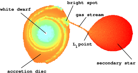
Figure 1: A non-magnetic CV.

1.1 The nature of the secondary stars in CVs

The spectral type and luminosity class of the secondary star in CVs can be estimated from basic theory, as follows. The mean density, ${\bar{\rho}}_{2}$, of the secondary star is given by

$${\bar{\rho}}_{2}={M_{2}\over{4\over 3}\pi R_{2}^{3}},$$ (1)

where $M_{2}$ and $R_{2}$ are the mass and volume radius (i.e. the radius of a sphere with the same volume as the Roche lobe) of the secondary star, respectively. The volume radius of the Roche lobe can be approximated by

$${{R_{2}}\over a}=0.47\biggl{(}{q\over{1+q}}\biggr{)}^{1/3}$$ (2)

smith98a , where $q=M_{2}/M_{1}$ and $a$ is the distance between the centres of mass of the binary components. Newton’s generalisation of Kepler’s third law can be written as

$${{4\pi^{2}a^{3}}\over GP^{2}}=M_{1}+M_{2}=M_{2}\biggl{(}{{1+q}\over q}\biggr{)},$$ (3)

where $P$ is the orbital period of the binary. Combining equations 1, 2 and 3 gives the mean density-orbital period relation,

$${\bar{\rho}}_{2}=105\,P^{-2}{\rm\ (h)}{\ \ \ \rm g\ cm}^{-3},$$ (4)

which is accurate to $\sim$6 per cent eggleton83 over the range of mass ratios relevant to most CVs ($0.01<q<1$). Most CVs have orbital periods of $1.25{\rm\ h}<P<9{\rm\ h}$, resulting in mean densities of $67{\rm\ g\,cm}^{-3}<{\bar{\rho}}_{2}<1.3{\rm\ g\,cm}^{-3}$. Such mean densities are typically found in M8V–G0V stars allen76 and hence the secondary stars in CVs should be similar to M, K or G main-sequence dwarfs. With a few caveats, this prediction is largely confirmed by observation smith98a ,beuermann98 .

1.2 Why image the secondary stars in CVs?

Even though we have just shown that most CV secondary stars are similar to lower main-sequence stars in their gross properties, it is not clear that they should share the same detailed properties. This is because CV secondaries are subject to a number of extreme environmental factors to which isolated stars are not. Specifically, CV secondaries are:

1. situated $\sim 1R_{\odot}$ from a hot, irradiating source (see smith95 );

2. rapidly rotating ($v_{rot}\sim 100$ km s^-1);

3. Roche-lobe shaped;

4. losing mass at a rate of $\sim 10^{-8}-10^{-11}M_{\odot}$ yr^-1;

5. survivors of a common-envelope phase during which they existed within the atmosphere of a giant star, and

6. exposed to nova outbursts every $\sim 10^{4}$ yr.

In order to study the impact of some of these environmental factors on the detailed properties of CV secondary stars, surface images are required. Direct imaging is impossible, however, as typical CV secondary stars have radii of 400 000 km and distances of 200 parsecs, which means that to detect a feature covering 20 per cent of the star’s surface requires a resolution of approximately 1 micro-arcsecond, 10 000 times greater than the diffraction-limited resolution of the world’s largest telescopes. Astro-tomography is hence a necessity when studying surface structure on CV secondaries.

Obtaining surface images of CV secondaries has much wider implications, however, than just providing information on the detailed properties of these stars. For example, a knowledge of the irradiation pattern on the inner hemisphere of the secondary star in CVs is essential if one is to calculate stellar masses accurate enough to test binary star evolution models (see section 3.3.4). Furthermore, the irradiation pattern provides information on the geometry of the accreting structures around the white dwarf (see section 3.3.4). Perhaps even more importantly, surface images of CV secondaries can be used to study the solar-stellar connection. It is well known that magnetic activity in isolated lower-main sequence stars increases with decreasing rotation period (e.g. rutten87 ). The most rapidly rotating isolated stars of this type have rotation periods of $\sim 8$ hours, much slower than the synchronously rotating secondary stars found in most CVs. One would therefore expect CVs to show even higher levels of magnetic activity. There is a great deal of indirect evidence for magnetic activity in CVs – magnetic activity cycles have been invoked to explain variations in the orbital periods, mean brightnesses and mean intervals between outbursts in CVs (see warner95 ). The magnetic field of the secondary star is also believed to play a crucial role in angular momentum loss via magnetic braking in longer-period CVs, enabling CVs to transfer mass and evolve to shorter periods. One of the observable consequences of magnetic activity are star-spots, and their number, size, distribution and variability, as deduced from astro-tomography of CV secondaries, would provide critical tests of stellar dynamo models in a hitherto untested period regime.

2 Detecting the secondary stars in CVs

Detecting spectral features from the secondary stars in CVs is not easy. There are two main reasons for this. First, CVs are typically hundreds of parsecs distant, rendering the lower main-sequence secondary very faint. Second, the spectra of CVs are usually dominated by the accretion disc and the resulting shot-noise overwhelms the weak signal from the secondary star. The result is that, in the 1998 study of Smith and Dhillon  smith98a , only 55 of the 318 CVs with measured orbital periods had spectroscopically identified secondary stars.

The best secondary star detection strategy depends very much on the orbital period of the CV, as this approximately determines the spectral type of the secondary via the empirical relation

$$\begin{array}[]{rrrll}Sp(2)\,\,\,=&\,\,26.5&-\ 0.7&\ P({\rm h}),&P<4\,{\rm h}\\ &\pm\,\,0.7&\pm\,\,0.2&\\ &&&&\\ =&\,\,33.2&-\ 2.5&\ P({\rm h}),&P\geq 4\,{\rm h}\\ &\pm\,\,3.1&\pm\,\,0.5&\\ \end{array}$$ (5)

smith98a , where $Sp(2)$ is the spectral type of the secondary; $Sp(2)=0$ represents a spectral type of G0, $Sp(2)=10$ is K0 and $Sp(2)=20$ is M0. Longer period CVs therefore have earlier spectral-type secondaries, which generally contribute a greater fraction (typically $>$75 per cent) of the total optical/infrared light than the secondary stars found in shorter period CVs, which usually only contribute $\sim$10–30 per cent dhillon00 . Equation 5 can then be used in conjunction with a black-body approximation to the wavelength, $\lambda_{\rm max}$, of the peak flux, $f_{\nu}$, for a star of effective temperature $T_{\rm eff}$,

$$\lambda_{\rm max}=5100/T_{\rm eff}\ \ \ \mu{\rm m},$$ (6)

to obtain a crude idea of the optimum observation wavelength required to detect the secondary star in a CV of known orbital period. With $T_{\rm eff}$ ranging from $\sim$6000–2000 K for the G–M dwarf secondary stars found in most CVs, $\lambda_{\rm max}$ ranges from $\sim$0.8–2.5 $\mu$m, i.e. the optimum wavelength always lies in the optical and near-infrared. In practice, when observing the secondary stars in longer-period CVs it is generally best to observe the numerous neutral metal absorption lines in the R-band around H$\alpha$ (e.g. drew93 ; bottom-right, figure 2), whereas short and intermediate-period secondaries are best observed via the TiO molecular bands and Na I absorption doublet in the I-band (e.g. wade88 ; top-right, figure 2). If optical spectroscopy fails to detect the secondary star in a CV, as is often the case in the shortest-period dwarf novae and the novalikes (which have very bright discs), it is possible to use near-infrared spectroscopy in the J-band littlefair00a and K-band (e.g. dhillon00 ); the brighter background in the near-infrared is offset to some extent by the greater line flux from the secondary star at these wavelengths (e.g. littlefair00b ; top-left, figure 2). In addition to absorption-line features, emission-line features from the secondary star are sometimes visible in CV spectra, especially in dwarf novae during outburst and novalikes during low-states (e.g. dhillon94 ; bottom-left, figure 2). These narrow, chromospheric emission lines originate on the inner hemisphere of the secondary star and are most probably due to irradiation from the primary and its associated accretion regions. The emission lines are usually most prominent in the Balmer lines, but have also been observed in He I, He II and Mg II (e.g. harlaftis99 ).

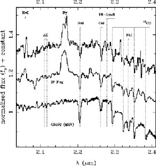
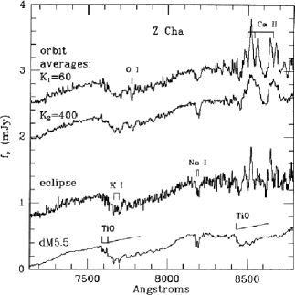
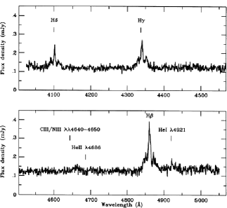
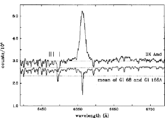
Figure 2: Secondary star features in CV spectra. Clockwise from top-left: IP Peg littlefair00b , Z Cha wade88 , DX And drew93 and DW UMa dhillon94 .

2.1 Skew mapping

If the secondary star is not visible in a single spectrum of a CV, one might naturally think that co-adding additional spectra will increase the signal-to-noise and hence increase the chances of a detection. This is true, but only if the additional spectra are first shifted to correct for the orbital motion of the secondary star, as otherwise the weak features will be smeared out. The problem is that the orbital motion is not known in advance; the solution is to use a technique known as skew mapping smith93 .

The first step is to cross-correlate each spectrum to be co-added with a template, usually the spectrum of a field dwarf of matched spectral type, yielding a time-series of cross-correlation functions (CCFs). If there is a strong correlation, the locus of the CCF peaks will trace out a sinusoidal path in a ‘trailed spectrum’ of CCFs, in which case plotting the velocity of each of the CCF peaks versus orbital phase allows one to define the secondary star orbit. More often, however, the CCFs are too noisy to enable well-defined peaks to be measured. Instead, the trailed spectrum of CCFs is back-projected in an identical manner to that employed in standard Doppler tomography marsh00 to produce what is known as a skew map. Any noisy peaks in the trailed spectrum of CCFs which lie along the true sinusoidal path of the secondary star will re-inforce during the back projection process, resulting in a spot on the skew map at ($0,K_{2}$), where $K_{2}$ is the radial-velocity semi-amplitude of the secondary star.

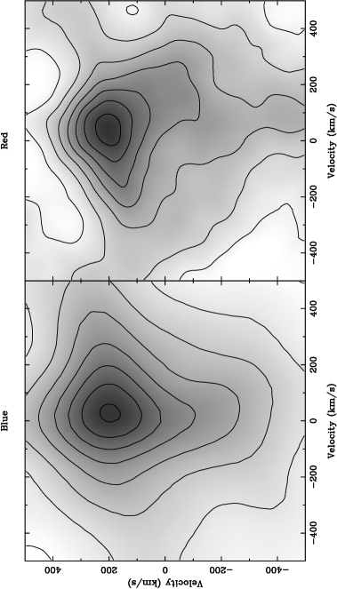
Figure 3: Skew maps of the old nova BT Mon smith98b .

Figure 3 shows an example of the successful use of the skew mapping technique applied to the old nova BT Mon smith98b . The value of $K_{2}$ determined from the skew map (205 km s^-1) was used to produce a co-added spectrum which enabled the rotational broadening and spectral type of the secondary star to be accurately determined. These system parameters were then used to calculate the distance and the component masses of BT Mon, which provide fundamental input to thermonuclear runaway models of nova outbursts. Although a powerful technique which is invaluable in the detection of faint secondary stars in CVs, skew mapping does not, however, provide surface images. To do this, other techniques are required, which we shall turn to now.

3 Mapping the secondary stars in CVs

The secondary stars in CVs are three-dimensional objects. Time-series of astronomical data, however, are effectively one-dimensional (in the case of light curves) or two-dimensional (in the case of spectra). The problem of obtaining surface images of CV secondaries is hence poorly constrained (see rice89 ), especially if one is restricted to the so-called one-dimensional case. We will begin the description of CV secondary mapping techniques by looking at the one-dimensional techniques. These include photometric light curve fitting, but also include methods where spectral information is parameterised in some way and the resulting values are then used to obtain surface images; radial-velocity curve fitting, line-flux fitting and line-width fitting all fall into this latter category. We will then look at the special case of Doppler tomography, which uses two-dimensional data to map two-dimensional structures. This means that Doppler tomography is fully constrained, but it also means that the secondary star is effectively compressed along the direction defined by the rotation axis into only two dimensions. Finally, we will look at potentially the most powerful technique – Roche tomography – which is very similar to the single-star mapping techniques described elsewhere in this volume cameron00 ,donati00 and which uses two-dimensional data to construct three-dimensional surface images of CV secondaries.

3.1 One-dimensional techniques

3.1.1   Radial-velocity curve fitting

If the centre-of-light and centre-of-mass of the secondary are not coincident, the star’s radial-velocity curve will be distorted in some way from the pure sine wave which represents the motion of the centre-of-mass. The observed radial-velocity curves of CV secondaries suffer from this distortion, due to both geometrical effects caused by the Roche-lobe shape and non-uniformities in the surface distribution of the line strength due to, for example, irradiation. Davey and Smith davey92 ,davey96 introduced an inversion technique which exploits this effect and uses the asymmetries present in observed radial-velocity curves to produce surface images of CV secondaries. Their ‘one-spot’ model assumed a single region of heating on the inner hemisphere of the secondary star which was allowed to vary in strength, size and position, i.e. there were 3 free parameters. The position of the spot, however, was restricted to vary in only the longitudinal direction, and hence the resulting maps assume symmetry about the orbital plane and are only two-dimensional.

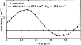
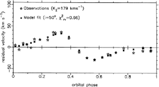
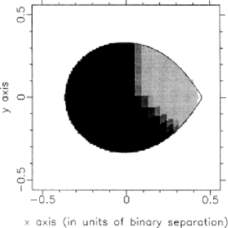
Figure 4: Radial-velocity curve fitting of the polar AM Her. Upper-left: Radial-velocity curve of the Na I absorption doublet around 8190Å davey92 . Lower-left: Residual-velocity curve, i.e. the motion of the centre-of-mass of the secondary has been removed davey96 . Right: Surface map of AM Her – the light region is where the Na I doublet is weakest davey96 .

Davey and Smith have successfully applied their technique to four dwarf novae and one polar davey92 ,smith95 ,davey96 . The surface image they derived of the polar AM Her is shown in the right-hand panel of figure 4. It can be seen that there is a general reduction in the line strength on the inner hemisphere of the secondary, a result consistent with the effects of heating caused by irradiation brett93 . It can also be seen that the line absorption is stronger on the leading hemisphere (the lower edge of the map in figure 4) than it is on the trailing hemisphere (the upper edge of the map in figure 4). This asymmetry has been interpreted as due to the gas stream blocking the radiation produced in the magnetic accretion column close to the white dwarf, thereby shielding an area on the leading hemisphere of the secondary star from irradiation. A similar asymmetry, but in the opposite sense (i.e. the trailing hemisphere has stronger line absorption than the leading hemisphere), has also been seen in the dwarf novae mapped by Davey and Smith smith95 . In these objects, however, there is an accretion disc instead of an accretion column. Irradiation by the bright-spot is apparently insufficient to account for the observed asymmetry davey92 , and so Davey and Smith speculated that circulation currents induced by the irradiation spreads the heating over a larger area, but preferentially towards the leading hemisphere due to coriolis effects. This idea was later confirmed by SPH modelling martin95 .

3.1.2   Light-curve fitting

Light-curve fitting is now a well-established tool in CV research, having found particular success in the study of accretion discs via the eclipse mapping method horne85 ,baptista00 . The brightness of the secondary star in eclipse mapping is, however, either completely ignored or included in the fit as a single nuisance parameter rutten94a . In order to obtain surface images of CV secondaries via light-curve fitting, it is necessary to extend the eclipse mapping method by constructing a secondary star grid of tiles in addition to, or instead of, an accretion disc grid and fit the whole light curve rather than just the eclipse portion. Each element in the grid is assigned an intensity, which is weighted according to its projected area and limb darkening at each orbital phase. A model light curve is then derived by summing the weighted intensities as a function of orbital phase. By comparing the model light curve for some grid brightness distribution with the observed light curve, the element intensities can be iteratively adjusted until the observed light curve is optimally fitted, usually using the maximum-entropy approach described in section 3.3.1.

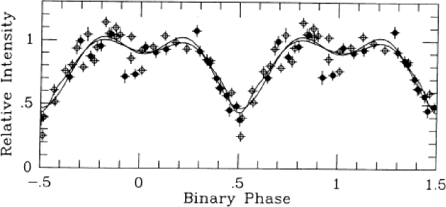
Figure 5: Ellipsoidal variations in the dwarf nova Z Cha wade88 .

Such an approach has been adopted by Wade and Horne wade88 , who used a secondary star grid, but no accretion disc grid, to fit the TiO band-flux light curve of the dwarf nova Z Cha. The observed data is represented by the points in figure 5 and their fits to the data are represented by the solid lines. The observed data show a double-humped variation, known as an ellipsoidal modulation. This is due to the changing aspect of the secondary’s Roche-lobe which presents the largest projected area, and hence highest flux, at quadrature (phases 0.25 and 0.75) and the smallest project area, and hence lowest flux, during conjunction (phases 0 and 0.5). The best fit to the data was obtained with a TiO distribution which has a minimum around the $L_{1}$ point and rises smoothly to a level 3 times higher on the hemisphere facing away from the white dwarf. This surface variation is consistent with the effects of irradiation brett93 and was used to correct the radial-velocity curves for the effects of a mis-match between the secondary’s light centre and its centre-of-mass in order to derive accurate stellar masses.

Wade and Horne wade88 did not include an accretion disc grid in their light-curve fits because the disc does not contribute to the TiO band-flux. Broad-band light curves, however, especially those obtained in the infrared, have approximately equal contributions from the disc and secondary, which means that any light-curve fitting must include both a secondary star grid and an accretion disc grid. Rutten rutten98 has developed such a technique, known as 3D eclipse mapping. The upper-left panel of figure 6 shows a typical accretion disc and secondary star grid used in 3D eclipse mapping. A secondary star with a luminous inner hemisphere and dark outer hemisphere, combined with a standard $T_{\rm eff}^{4}\propto R_{\rm disc}^{-3}$ disc warner95 , produces the light curve shown in the right-hand panel of figure 6. Fitting this light curve produces the map of the system shown in the lower-left panel of figure 6, which is a good representation of the original intensities assigned to the grid elements. 3D eclipse mapping has only recently been applied to real data groot99 , however, and awaits full exploitation in secondary star studies.

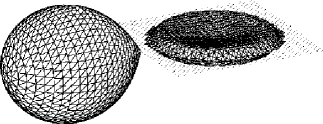
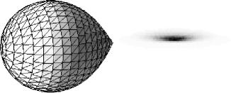
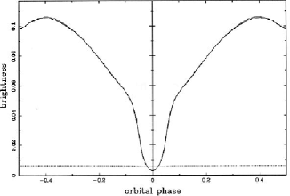
Figure 6: 3-D eclipse mapping rutten98 .

3.1.3   Line-width fitting

We have just seen how variability in two of the ‘integral’ properties of a line profile, the line strength and the line position, can be used to map the secondary stars in CVs. There is, however, a third integral property of line profiles which can be used to deduce surface images – the variability in line width, or more generally, in line shape. The reason line width varies with orbital phase can be understood by recalling that the secondary stars in CVs are synchronously rotating and geometrically distorted, which results in a variation in the projected radius of the secondary as a function of orbital phase. For a given orbital period, the larger the projected radius of the secondary the broader the line profile will be, which means that the rotational broadening varies with orbital phase. At the conjunction phases, the projected radius and rotational broadening are at a minimum, while at quadrature they are at a maximum.

The observed variations in rotational broadening also depend on the inclination of the binary plane and the surface distribution of line strength. Casares et al. casares96 exploited this effect in order to determine the inclination of the magnetic novalike AE Aqr. By constructing a secondary star with essentially no surface structure, other than that due to an assumed gravity darkening law, they calculated a grid of model rotational-broadening curves which were then matched to the observed curve using a $\chi^{2}$-test. Shahbaz shahbaz98 , also motivated by a desire to determine inclination angles, added an extra dimension by fitting the line shape rather than just the line width. Both of these techniques are examples of model fitting, in which any surface structure must be added to the model in an ad-hoc manner prior to fitting. A better approach to mapping surface structure is image reconstruction, in which the intensity of each image pixel is a free parameter; Roche tomography is an example of such a technique (see section 3.3).

3.2 Doppler tomography

Doppler tomography uses a time-series of emission line profiles spanning the binary orbit to construct a two-dimensional map of the system in velocity space. Although primarily used as a tool to study the accretion regions in CVs, Doppler tomography has also proved to be remarkably successful in secondary star studies. This is because Doppler tomography provides a way of cleanly separating the emission component due to the secondary star from the broader and often stronger emission originating in the accretion regions. The technique and some of its most important achievements to date are reviewed elsewhere in this volume marsh00 ,schwope00 . In this section, we highlight one particularly important example of the application of Doppler tomography to the study of CV secondaries – the work of Steeghs et al. steeghs96 on the dwarf nova IP Peg during outburst (figure 7).

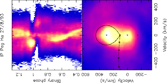
Figure 7: A slingshot prominence and accretion disc shadow in the dwarf nova IP Peg steeghs96 .

The upper panel of figure 7 shows the observed trailed spectrum of the H$\alpha$ emission line in IP Peg. Note the stationary component at 0 km s^-1 running the entire length of the time-series and the narrow sinusoidal component which crosses from red-shifted to blue-shifted around phase 0.5. The sinusoidal emission component is mapped onto the inner hemisphere of the secondary star’s Roche lobe (lower panel, figure 7). This emission is almost certainly being powered by irradiation from the white dwarf and the hot, inner regions of the outbursting accretion disc, a conclusion supported by the fact that the emission appears to be stronger around the poles than it is around the $L_{1}$ point, implying that obscuration of the inner disc by the flared, outer disc might be occurring. The stationary component is mapped onto the centre-of-mass of the binary, indicated by the cross at zero velocity in the lower panel of figure 7. This component is much more difficult to explain as there is no obvious part of the binary system which is at rest. One possible interpretation is that the emission is due to material trapped in a ‘slingshot prominence’, a magnetic loop originating on and co-rotating with the secondary. With this model, Steeghs et al. steeghs96 used the Doppler map in figure 7 to estimate the magnetic field strength of the secondary star ($\sim$ kG) and the temperature (2 $\times$ 10⁴ K) and total mass ($\sim$10¹⁸ g) of the material in the prominence, and found good agreement with the parameters deduced from similar prominences observed in isolated dwarf stars (e.g. cameron89 ).

3.3 Roche tomography

Roche tomography rutten94b ,watson00 takes as its input a trailed spectrum, i.e. a time-series of spectral-line profiles, and provides on output a map of the secondary star in three-dimensions. The main advantage of Roche tomography over the one-dimensional techniques described in section 3.1 is that the one-dimensional techniques each extract and then use just one piece of information about the line profile (e.g. the variation in its flux, radial velocity or width) to map the secondary star, whereas Roche tomography uses all of the information in the line profile, as described in section 3.3.1.

Roche tomography is very similar to the Doppler imaging technique used to map single stars (e.g. cameron00 ,donati00 ), contact binaries maceroni94 and detached secondaries in pre-CVs ramseyer95 . In fact, Roche tomography and Doppler imaging of single stars differ in only two fundamental ways. First, the secondary stars in CVs are tidally-distorted into a Roche-lobe shape and are in synchronous rotation about the binary centre-of-mass; isolated stars rotate only about their own centre-of-mass and are symmetric about their rotation axis. Second, the continuum is ignored in Roche tomography, whereas it is included in Doppler imaging. This is because of the variable and unknown contribution to the spectrum of the accretion regions in CVs, forcing Roche tomography to map absolute line fluxes. The data are therefore slit-loss corrected and then continuum-subtracted prior to mapping with Roche tomography, whereas when Doppler imaging the spectra need not be slit-loss corrected and the continuum is divided into the data.

Although the system parameters are generally better constrained in CVs than they are in single stars, Roche tomography is a much harder task than Doppler imaging. This is because CV secondaries are usually both fainter and more rapidly rotating than isolated stars, resulting in surface images of a much lower quality than are routinely obtained via Doppler imaging (see section 3.3.4).

3.3.1   Principles and practice

In Roche tomography, the secondary star is modelled as a grid of quadrilateral surface elements of approximately equal area lying on the critical potential surface which defines the Roche lobe. Each surface element, or tile, is then assigned a copy of the local specific intensity profile convolved with the instrumental resolution. These profiles are then scaled to take into account phase dependent effects, such as variations in the projected area, limb darkening and obscuration and Doppler-shifted according to the radial velocity of the surface element at a particular phase. Simply summing up the contributions from each element gives the rotationally broadened profile at any particular phase. An example of this ‘forward’ process is shown in figure 8, which shows the trailed spectrum resulting from a secondary star with a uniformly radiating inner hemisphere.

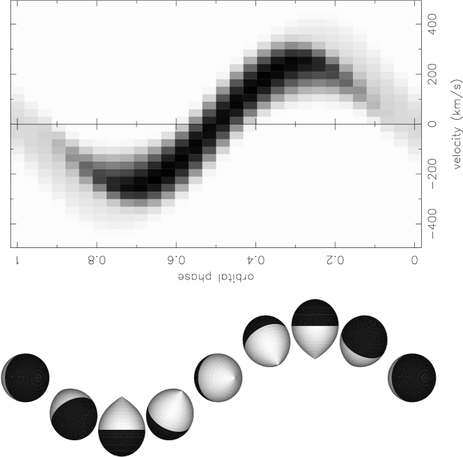
Figure 8: The principles of Roche tomography.

By iteratively varying the strengths of the profile contributed by each tile it is possible to perform the ‘inverse’ process and obtain the map which fits the observed data. How well the map fits the observed data is defined by a consistency statistic, given by the reduced chi-squared:

$${\chi}^{2}={1\over n}\sum_{i=1}^{n}\left({p_{i}-o_{i}}\over{\sigma_{i}}\right)^{2},$$ (7)

where $n$ is the number of data points, $p_{i}$ and $o_{i}$ are the predicted and observed data, and $\sigma_{i}$ is the error on $o_{i}$. Fitting the data as closely as possible (i.e. minimising $\chi^{2}$) is not a good approach, however, as noise will dominate the resulting map. A better approach is to reduce $\chi^{2}$ until the observed and predicted data are consistent, i.e. $\chi^{2}\sim 1$. Such a condition is satisfied by many maps, however, and so a regularisation statistic is employed to select just one of them. Following Horne horne85 , we select the ‘simplest’ map, which is given by the map of maximum entropy. The definition of entropy, $S$, that we use is

$$S=\sum_{j=1}^{k}m_{j}-d_{j}-m_{j}\ln\left(m_{j}/d_{j}\right),$$ (8)

where $k$ is the number of tiles in the map, and $m_{j}$ and $d_{j}$ are the map and the so-called ‘default map’, respectively. Equation 8 shows that the entropy is a measure of the similarity of the map to the default map and hence it is the default map which defines what we mean by the ‘simplest’ image. The choice of default map is therefore of great importance. We have experimented with a number of different prescriptions for the default map watson00 . The two most successful have been a uniform default, where every tile in the default is set to the average value in the map, and a smoothed version of the map, achieved using a Gaussian blurring function. In the former case, we are selecting the most uniform map consistent with the data, which constrains large-scale surface structure, and in the latter case we are selecting the smoothest map consistent with the data, which constrains short-scale structure. An efficient algorithm for the task of maximising entropy subject to the constraint imposed by $\chi^{2}$ is given by Skilling and Bryan skilling84 and has been implemented by them in the fortran package memsys.

3.3.2   Assumptions

The basic assumptions which underlie Roche tomography are:

1. The secondary star is Roche-lobe filling, synchronously rotating and in a circular orbit.

   These are believed to be valid assumptions because there is ample evidence for mass transfer and the synchronisation and circularisation timescales are both insignificant compared to the lifetime of a CV warner95 .

2. The observed surface of the star coincides with the surface defined by the critical Roche potential.

   The observed surface of a typical CV secondary (i.e. where the absorption lines originate) lies at a potential corresponding to a star that fills 99.97 per cent of its Roche lobe, which gives a change of less than 1 per cent in the shape of the line profile shahbaz98 .

3. The shape of the intrinsic line profile remains unchanged.

   Only the flux of the intrinsic line profile is allowed to vary. This assumption is valid because the rotational broadening usually dominates over intrinsic broadening. Moreover, it should be possible to identify errors in the intrinsic line-profile shape by the artifacts they induce in the reconstructions (see section 3.3.3).

4. The line profile is due to secondary star light only.

   The accretion disc is typically too hot to contribute to the cool stellar features. Furthermore, any accretion disc component present in a spectral line is usually instantly recognisable due to its extreme width and anti-phased radial-velocity motion.

5. The secondary star exhibits no intrinsic variation during the observation.

   The surface features of the secondary star might change during an observation due to, for example, a flare. This will result in artifacts in the maps, as discussed in section 3.3.3.

6. The orbital period, inclination, stellar masses, limb darkening, intrinsic line profile and systemic velocity are known.

   The orbital period of a CV is usually precisely known. The other parameters are more uncertain – we explore how errors in them affect the reconstructions in section 3.3.3.

7. The final map is the one of maximum entropy (relative to an assumed default image) which is consistent with the data.

   The data constrains the final map through the consistency statistic, $\chi^{2}$. The default map constrains the final map through the regularisation statistic, $S$. If the data are noisy, the data constraints will be weak and the map will be strongly influenced by the default map. If the data are good, however, the image will not be greatly influenced by the default and the choice of default makes little difference to the final map. The default may thus be regarded as containing prior information about the map, and the map will be modified only if the observations require it. The importance of this assumption therefore depends on the quality of the data.

3.3.3   Errors

The maps resulting from any form of astro-tomography are prone to both systematic errors, due to errors in the assumptions underlying the technique, and statistical errors, due to measurement errors on the observed data points. It is essential that the effects of these errors on the reconstructions are quantified in order to properly assess the reality of any surface structure present. This is especially true of Roche tomography, for which the input data is generally noisier due to the faintness of CV secondaries, a problem further exacerbated by the fact that noise in Roche tomograms can mimic the appearance of star-spots watson00 .

We begin by discussing our approach to statistical error determination watson00 . The maximum-entropy technique is non-linear, in the sense that each map value is not a linear function of the data values. This makes it very difficult to propagate the statistical error on a data point through the maximum-entropy process in order to calculate the statistical error on each tile of the map. Furthermore, the statistical errors on each tile will not be independent due to, for example, the projection of bumps in the line profiles across arcs of constant radial velocity on the secondary star (see figure 9). The simplest approach to error estimation, in this case, is to use a Monte Carlo-based simulation.

Monte-Carlo techniques rely on the construction of a large (typically hundreds, in the case of Roche tomography) sample of synthesized datasets which have been effectively drawn from the same parent population as the original dataset, i.e. as if the observations have been repeated many hundreds of times. This large sample of synthesized datasets is then used to create a large sample of Roche tomograms, resulting in a probability distribution for each tile in the map. The main difficulty with this technique, aside from the demands on computer time, lies in the construction of the sample of synthesized datasets. One approach (e.g. rutten94a ) is to ‘jiggle’ each data point about its observed value, by an amount given by its error bar multiplied by a number output by a Gaussian random-number generator with zero mean and unit variance. This process adds noise to the data, however, which means that the synthesized datasets are not being drawn from the same parent population as the observed dataset – noise is being added to a dataset which has already had noise added to it during the measurement process. In practice, this means that fitting the sample datasets to the same level of $\chi^{2}$ as the original dataset is either impossible (i.e. the iteration does not converge) or results in maps dominated by noise, which overestimates the true error on each tile.

A much better approach to creating synthesized datasets is the bootstrap method efron82 , which we have implemented as follows watson00 . From our observed trailed spectrum containing $n$ data points, we select, at random and with replacement, $n$ data values and place them in their original positions in the new, synthesized trailed spectrum. Some points in the synthesized trailed spectrum will be empty, in which case they will be omitted from the fit; in practice, this is achieved by setting the error bars on these points to infinity. Other points in the synthesized trailed spectrum will have been selected once or more, in which case their error bars are divided by the square root of the number of times they were picked. The advantage of bootstrap resampling over jiggling is that the data is not made noisier by the process as only the errors bars on the data points are manipulated. It is therefore possible to fit the synthesized trailed spectra to the same level of $\chi^{2}$ as the observed data, giving a much more reliable estimate of the statistical errors in the maps. The bootstrap method has been shown to work very effectively with Roche tomography watson00 , and we present an example of its application in figures 11 and 13.

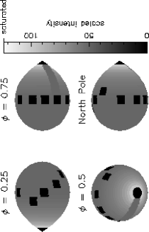
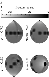
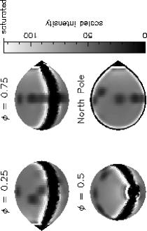
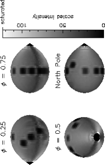
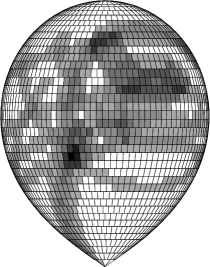
Figure 9: Systematic errors in Roche tomography watson00 . Top row: The test image (left) and the best fit (right). Middle row: Equatorial banding due to the effect of an incorrect systemic velocity (left) and incorrect limb darkening (right). Bottom row: Ring-like streaks due to the effects of phase undersampling (left), which correspond to lines on the secondary star with the same radial velocities as the spots (right).

The determination of systematic errors requires a completely different approach to that employed for the determination of statistical errors. We have approached systematic errors in Roche tomography watson00 in much the same way that Marsh and Horne marsh88a explored them in Doppler tomography. We first constructed a test image (top-row, left, figure 9) of the secondary star containing all of the surface features we might expect to find when mapping real data. These include irradiation, shadowing by the gas stream and star-spots covering a range of latitudes and longitudes. We used the test image to create a test trailed spectrum which we then fit using Roche tomography to reconstruct the surface image of the star. As can be seen from figure 9 (top-row, right), the best fit reproduces all of the features in the test image. We then explored the effects of systematic errors on the reconstruction by varying the input parameters to Roche tomography and re-fitting the test trailed spectrum. In this way we explored how variations in the systemic velocity, limb darkening, inclination, velocity smearing, phase undersampling, noise, intrinsic line profile, resolution, default map, stellar masses and stellar flares affect the reconstructions watson00 .

We find that systematic errors in Roche tomography generally result in only two major artifacts in the Roche tomograms: ring-like streaks and equatorial banding watson00 . Equatorial banding results whenever there is a mis-match between the maximum velocities present in the line profile and the maximum velocities available on the secondary star grid, which occurs whenever the wrong systemic velocity, limb darkening, inclination, velocity smearing, intrinsic line profile or stellar masses are used in the reconstruction. The banding occurs around the equator of the star because this is where the highest radial velocities are found. Some examples of equatorial banding patterns in Roche tomograms are shown in figure 9, where the maps have been reconstructed using incorrect values for the systemic velocity (middle row, left) and limb darkening (middle row, right).

Ring-like streaks appear in Roche tomograms when one or a few of the spectra in the input data dominate. This occurs when there is phase undersampling, for example, or when there is a flare in the data at a particular phase. The effect is analogous to the streaks observed in Doppler tomography marsh88a and can be understood by considering that lines of constant radial velocity on the secondary star at a particular phase can be integrated along to construct a line profile. These lines of constant radial velocity are ring-like in shape and if there are only a few phases, or if the profile is particularly bright at a certain phase, the streaks will not destructively interfere, leaving ring-like artifacts on the Roche tomogram. An example of a Roche tomogram reconstructed using only 5 orbital phases is shown in figure 9 (bottom row, left). The streaks present in this image correspond to lines on the secondary star with the same radial velocity as the spots, as shown at phase 0.25 in figure 9 (bottom row, right).

The error experiments presented here show that any feature on a Roche tomogram must be subjected to two tests before its reality can be confirmed. The first test is to determine whether the feature is statistically significant and is performed via a Monte-Carlo technique with bootstrap-resampling. The second test is to compare the feature with the appearance of known artifacts of the technique due to errors in the underlying assumptions, such as those presented in figure 9. If a surface feature survives both of these tests unscathed, it can be assumed to be real.

3.3.4   Results

Roche tomograms currently exist for only 3 CVs: the novalike DW UMa rutten94b , the dwarf nova IP Peg rutten96 and the polar AM Her davey96 . In this section we will present two new Roche tomograms – the polar HU Aqr and an improved study of IP Peg.

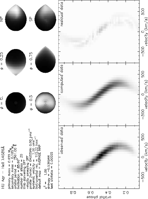
Figure 10: Roche tomogram of the polar HU Aqr.

Figure 11: A slice through the secondary star in HU Aqr.

The Roche tomogram of HU Aqr in the light of the He II $4686$Å emission line observed by Schwope et al. schwope97 is shown in figure 10, where bright regions in the map represent areas where the emission line flux is at its strongest. There are two main features in the Roche tomogram – the strong asymmetry between the inner (phase 0.5) and outer (phase 0) hemispheres of the secondary and a weaker asymmetry between the leading (phase 0.75) and trailing (phase 0.25) hemispheres of the secondary. The reality of the latter asymmetry can be assessed from figure 11, which shows a slice passing through the leading hemisphere (LH), north pole (NP), trailing hemisphere (TH)and south pole (SP) of the secondary star. The triangular points represent the map values, and it can be seen that the leading hemisphere is a factor of two fainter than the trailing hemisphere. The significance of this difference can be assessed from the curves in figure 11, which show confidence limits on the map values derived from 200 bootstrap resampling experiments; 67 per cent of the map values (measured relative to the mode of the distribution) lie within the range bounded by the solid curves and 100 per cent of the map values lie within the range bounded by the dotted curves. Figure 11 shows that we can be 100 per cent certain that the asymmetries between the trailing and leading hemispheres are not due to statistical errors. Furthermore, none of the systematic errors explored in section 3.3.3 result in asymmetries of the type observed in figure 10, implying that the asymmetries are real. Schwope et al. schwope97 reached a similar conclusion based on a model-fitting technique. They attributed the asymmetry between the inner and outer hemispheres to irradiation by the magnetic accretion column and the asymmetry between the leading and trailing hemispheres to shielding of this irradiation by the gas stream.

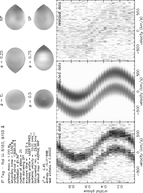
Figure 12: Roche tomogram of the dwarf nova IP Peg.

Figure 13: A slice through the secondary star in IP Peg.

The Roche tomogram of IP Peg in the light of the Na I absorption doublet around 8190Å is presented in figure 12, where bright regions in the map represent areas where the flux deficit is at its largest, i.e. where the absorption line is at its strongest. The most noticeable feature in the map is the asymmetry between the inner (phase 0.5) and outer (phase 0) hemispheres, which is slightly skewed towards the leading edge (phase 0.75) of the secondary. As described in section 3.1.1, this can be attributed to the effect of irradiation by the accretion regions and the resulting circulation currents on the secondary. There is another feature of note in the tomogram of figure 12 – a spot on the leading edge of the secondary. The spot is bright, which means it is an area that exhibits stronger Na I absorption. This is not consistent with what one might expect from a star-spot, because it is known that the Na I flux deficit decreases with later spectral type brett93 and star-spots are generally believed to be of order 1000 K cooler than the surrounding photosphere vogt81 (although spots hotter than the photosphere have also been imaged donati92 ). An inspection of the confidence limits in a slice through the spot (figure 13), however, shows that the feature is not statistically significant; the spot is the hump at ‘LH’ in figure 13 and it can be seen that the 67 per cent confidence limits widen significantly around it.

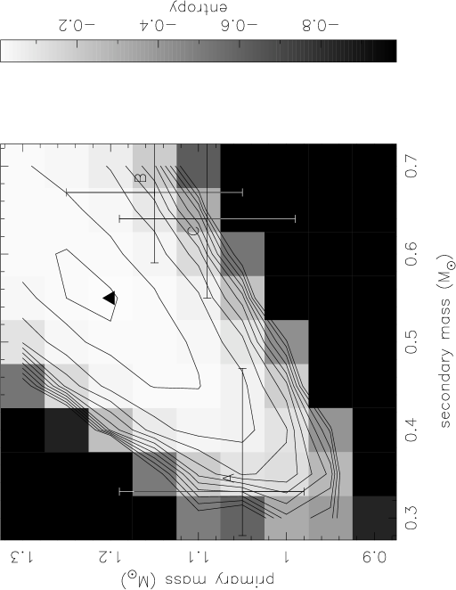
Figure 14: Entropy landscape for IP Peg.

Although we have not, unfortunately, imaged a star-spot in IP Peg, we can use the Roche tomogram to derive accurate values for the masses of the stellar components. As discussed in section 3.3.3, using incorrect values for stellar masses results in equatorial banding, which increases the entropy of the reconstructions when using a uniform default map. The masses (and inclinations consistent with the masses and the observed eclipse width) can therefore effectively be included in the fit by constructing an entropy landscape rutten94b ,rutten96 , which plots entropy as a function of the primary and secondary masses. The entropy landscape for IP Peg is shown in figure 14. The triangle denotes the point of highest entropy, corresponding to primary and secondary masses of $M_{1}=1.2$ M_⊙ and $M_{2}=0.55$ M_⊙. These values are in approximate agreement with the mass determinations of Beekman et al. beekman00 , Martin et al. martin89 and Marsh marsh88b , marked $A$, $B$ and $C$ in figure 14. Because the masses derived from an entropy landscape automatically account for the geometrical distortion of the secondary and any non-uniformities in its surface structure, the technique provides very tightly constrained mass determinations, particularly in directions orthogonal to the diagonal feature in figure 14 (corresponding to mass ratios that allow the radial velocity of the secondary’s centre-of-mass to remain constant).

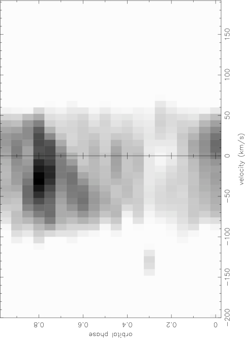
Figure 15: Trailed spectrum of SS Cyg derived using LSD shahbaz00 .

4 Conclusions

The Roche tomogram of IP Peg presented in figure 12 represents the best that can be obtained with a 4-m class telescope when mapping a single spectral line. Yet even this does not appear to be good enough to image the star-spots we might reasonably expect to be present on IP Peg’s secondary. To provide routine imaging of star-spots on CV secondaries it will therefore be necessary to move up to 8-m class telescopes and/or combine many spectral lines to increase signal-to-noise, using techniques such as least-squares deconvolution (LSD) donati97 . An initial attempt at LSD using data on the dwarf nova SS Cyg is presented in figure 15 and appears to show the tell-tale signature of a star-spot – the diagonal stripe moving from blue to red velocities between phases 0.5–0.8. These data require more careful reduction before they can be mapped, but it is clear that LSD is the way forward and we can expect the first star-spots on CV secondaries to have been unambiguously imaged by the time the next conference on astro-tomography convenes.

References

- (1) C. W. Allen: Astrophysical Quantities (Athlone Press, London 1976)
- (2) R. Baptista: this volume
- (3) G. Beekman, M. Somers, T. Naylor, C. Hellier: MNRAS. in press
- (4) K. Beuermann, I. Baraffe, U. Kolb, M. Weichhold: A&A. 339, 518 (1998)
- (5) J. M. Brett, R. C. Smith: MNRAS. 264, 641 (1993)
- (6) J. Casares, M. Mouchet, I. G. Martinez-Pais, E. T. Harlaftis: MNRAS. 282, 182 (1996)
- (7) A. C. Cameron, R. D. Robinson: MNRAS. 238, 657 (1989)
- (8) A. C. Cameron: this volume
- (9) S. C. Davey, R. C. Smith: MNRAS. 257, 476 (1992)
- (10) S. C. Davey, R. C. Smith: MNRAS. 280, 481 (1996)
- (11) V. S. Dhillon, D. H. P. Jones, T. R. Marsh: MNRAS. 266, 859 (1994)
- (12) V. S. Dhillon, S. P. Littlefair, S. B. Howell, D. R. Ciardi, M. K. Harrop-Allin, T. R. Marsh: MNRAS. 314, 826 (2000)
- (13) J.-F. Donati, et al: A&A. 265, 682 (1992)
- (14) J.-F. Donati, M. Semel, B. D. Carter, D. E. Rees, A. C. Cameron: MNRAS. 291, 658 (1997)
- (15) J.-F. Donati: this volume
- (16) J. E. Drew, D. H. P. Jones, J. A. Woods: MNRAS. 260, 803 (1993)
- (17) B. Efron: The Jackknife, the Bootstrap and Other Resampling Plans (SIAM, Philadelphia 1982)
- (18) P. Eggleton: ApJ. 268, 368 (1983)
- (19) P J. Groot: Optical Variability in Compact Sources. PhD Thesis, University of Amsterdam (1999)
- (20) E. T. Harlaftis: A&A. 346, L73 (1999)
- (21) K. Horne: MNRAS. 213, 129 (1985)
- (22) S. P. Littlefair, V. S. Dhillon, S. B. Howell, D. R. Ciardi: MNRAS. 313, 117 (2000)
- (23) S. P. Littlefair, V. S. Dhillon, E. T. Harlaftis, T. R. Marsh: in preparation
- (24) C. Maceroni, O. Vilhu, F. van ’t Veer, W. Van Hamme: A&A. 288, 529 (1994)
- (25) T. R. Marsh, K. Horne: MNRAS. 235, 269 (1988)
- (26) T. R. Marsh: MNRAS. 231, 1117 (1988)
- (27) T. R. Marsh: this volume
- (28) J. S. Martin, D. H. P. Jones, M. T. Friend, R. C. Smith: MNRAS. 240, 519 (1989)
- (29) T. J. Martin, S. C. Davey: MNRAS. 275, 31 (1995)
- (30) T. F. Ramseyer, A. P. Hatzes, F. Jablonski: AJ. 110, 1364 (1995)
- (31) J. B. Rice, W. H. Wehlau, V. L. Khokhlova: A&A. 208, 179 (1989)
- (32) R. G. M. Rutten: A&A. 177, 131 (1987)
- (33) R. G. M. Rutten, V. S. Dhillon, K. Horne, E. Kuulkers: A&A. 283, 441 (1994)
- (34) R. G. M. Rutten, V. S. Dhillon: A&A. 288, 773 (1994)
- (35) R. G. M. Rutten, V. S. Dhillon: ‘Roche Tomography of the Cool Star in IP Peg’. In: CVs and Related Objects. ed. by A. Evans, J. H. Wood (Kluwer, Dordrecht, 1996) pp. 21–24
- (36) R. G. M. Rutten: A&AS. 127, 581 (1998)
- (37) A. D. Schwope, K.-H. Mantel, K. Horne: A&A. 319, 894 (1997)
- (38) A. D. Schwope: this volume
- (39) T. Shahbaz: MNRAS. 298, 153 (1998)
- (40) T. Shahbaz: private communication
- (41) J. Skilling, R. K. Bryan: MNRAS. 211, 111 (1984)
- (42) D. A. Smith, V. S. Dhillon: MNRAS. 301, 767 (1998)
- (43) D. A. Smith, V. S. Dhillon, T. R. Marsh: MNRAS. 296, 465 (1998)
- (44) R. C. Smith, A. C. Cameron, D. S. Tucknott: ‘Skew Mapping: A New Way to Detect Secondary Stars in CVs’. In: CVs and Related Physics. ed. by O. Regev, G. Shaviv (IoP, Bristol, 1993) pp. 70–72
- (45) R. C. Smith: ‘Secondary Stars and Irradiation’. In: Cape Workshop on Magnetic CVs. ed. by D. A. H. Buckley, B. Warner (ASP, San Francisco, 1995) pp. 417–426
- (46) D. Steeghs, K. Horne, T. R. Marsh, J.-F. Donati: MNRAS. 281, 626 (1996)
- (47) S. S. Vogt: ApJ. 250, 327 (1981)
- (48) R. A. Wade, K. Horne: ApJ. 324, 411 (1988)
- (49) B. Warner: Cataclysmic Variable Stars (CUP, Cambridge 1995)
- (50) C. A. Watson, V. S. Dhillon: in preparation.