A Detailed Two-Dimensional Stellar Population Study of M 32

Abstract

We present Integral Field Spectroscopy of the 9${}^{\prime\prime}\times$12^′′ circumnuclear region of M 32 obtained with the 2D_FIS fibre spectrograph installed at the 4.2m William Herschel Telescope. From these spectra line strength maps have been made for about 20 absorption lines, mostly belonging to the Lick system. We have found good agreement with long-slit line strength profiles in the literature. We find no radial gradients in the azimuthally averaged absorption line indices. We have fitted the mean values of each spectral index and colours from the literature for the inner regions of M 32 to the models of Vazdekis et al. (1996) and Worthey (1994) finding present data can be well interpreted for a single stellar population of an intermediate age ($\sim$4 Gyr) and a metallicity similar to solar (Z=0.02).

1 Introduction

Since M 32 is the brightest elliptical galaxy of the Local Group it has been studied extensively as a template for elliptical galaxies further away. Stellar population studies, aiming at constraining its formation and evolution include, for instance, Spinrad & Taylor (1969), Faber (1972), O’Connell (1980), Burstein et al. (1984), Freedman (1992), Rose (1994) and Dorman et al. (1995). The first of those studies showed that the stellar populations of M 32 are much bluer than those of giant ellipticals. O’Connell (1980) found that the spectrum of M 32 can be fitted with solar metallicity stars and argued that the last episode of star formation in this galaxy happened $\sim$ 5 Gyrs ago. This result has been confirmed by various authors, on the basis of a number of different stellar population models (e.g. Burstein et al. 1984; Rose 1985, 1994; Bica et al. 1990). This fact distinguishes this galaxy from most other ellipticals, which are found to be much older (e.g., O’Connell 1976, Aaronson et al. 1978, Tinsley 1980, Rose 1994, Vazdekis et al. 1997, Tantalo et al. 1998, Peletier et al. 1999, hereafter P99) but also from studies in which is obtained a wide range in age (González 1993, Jørgensen 1999, Vazdekis & Arimoto 1999, Trager et al. 2000). Very recently an extraordinary fit to a high signal-to-noise and high resolution blue spectrum of M 32 has been achieved by Vazdekis & Arimoto (1999) using a model spectrum corresponding to a luminosity-weighted mean stellar population of 4 Gyr and solar metallicity selected from the new single-age, single-metallicity (SSP) spectral library of Vazdekis (1999). The spectrum in the whole optical spectral range of M32, however, is not completely understood at present. When trying to fit all spectral features covering a large spectral range in detail, it seems that the galaxy cannot be fitted with a single-age, single-metallicity stellar population (see e.g. Burstein et al. (1984), who showed that H$\beta$ is considerably stronger than expected by their models (see also Faber et al. 1992)). Understanding these small discrepancies will lead to a better understanding of both the stellar populations of M 32, and of current-day stellar population models. For that reason the main aim of this paper is to present a large dataset of well-calibrated data for the central region of M32, and fit them to current, state-of-the-art stellar population models. Stellar population models of old stellar systems have evolved and matured significantly in the most recent years. Although still following the same concept as the models of Tinsley & Gunn (1976), Aaronson et al. (1978), Tinsley (1980), Arimoto and Yoshii (1986), they have improved considerably, thanks to new sets of isochrone calculated with improved input physics, including the advanced stages of stellar evolution such as the HB and the AGB (e.g., Bertelli et al. 1994; Dorman et al. 1995) and extensive photometric and spectral stellar libraries, either empirical or theoretical, which cover wide ranges in atmospheric parameters (e.g., Worthey et al. 1994, Lejeune et al. 1997). Since most of the current-day models (e.g., Worthey 1994, hereafter W94; Vazdekis et al. 1996, hereafter V96) make use of extensive libraries of empirical stellar spectra to predict absorption line-strengths at intermediate resolution (FWHM $\sim$ 9Å) in a well-defined system, i.e., the Lick system (Faber et al. 1985; Gorgas et al. 1993; Worthey et al. 1994; Worthey & Ottaviani 1997), it is now possible to study not only the ages and metallicities of the galaxies, but also their abundance ratios, which provide information about the physical conditions at the time of formation.

The data that we analyze here come from Integral Field Spectroscopy (IFS) of the central zone of M 32. For the first time for this galaxy 2-dimensional absorption line-strength maps of the inner regions were obtained, allowing us to analyze these indices radially and azimuthally. Maps were made for most of the Lick indices as well as the CaII IR triplet features of Díaz et al. (1989). For the interpretation of the data we have used the model of W94, the first one including line-strength predictions for the Lick system, and our own model (V96), which is based on the isochrones of Bertelli et al. (1994) and which make use of extended empirical stellar input libraries to calculate the stellar fluxes and the broadband colors instead of calculating them from the model stellar atmospheres. We do not find any noticeable line strength gradients for this galaxy. Although this is not surprising, given the fact that there is no evidence for colour gradients (Peletier 1993, Lauer 1998) in the inner regions, and for line strength gradients in previous work (e.g. Trager et al. 1998, hereafter T98, González 1993), there are very few other galaxies where colour and line strength profiles are so flat. The aim of this paper has also been to address this problem by investigating gradients in more line indices than before, using higher-quality data.

The organization of this paper is as follows. In § 2 we present these observations and the data reduction. In § 3 we fit the data to predictions from the stellar population synthesis model. The results are shown in § 4 while a discussion and our conclusions are presented in § 5 and § 6, respectively.

2 Observations and Data Reduction

The data were obtained on February 15 and 16 1997 at the Observatorio del Roque de los Muchachos on the Island of La Palma. We used the 2D-FIS (Two-dimensional Fiber ISIS System), which linked the f/11 Cassegrain focus of the 4.2m William Herschel Telescope (WHT) and the ISIS (Carter et al. 1993) double spectrograph. A detailed description is provided by García et al. (1994). The main characteristics of our setup are given in P99. In the blue arm, the R300 grating was used, giving us a reciprocal dispersion of 1.55 Å pixel^-1 (96 km s^-1), a spectral range between 4100 and 5650 Å, covering most of the lines of the Lick system, including H$\gamma$ (Worthey & Ottaviani 1997), and a resolution of 2 pixels. In the red, we centred our spectrum on the Ca II IR triplet. Here we had a pixel size of 28 km s^-1 (resolution 2 pixels) and a spectral range from 8200 to 9000 Å. On both arms 1024 $\times$ 1024 thinned TEK CCDs were used. A dichroic, centred at 6100 Å, was used, and in the red arm a GG495 order sorting filter was placed as well. Weather conditions were photometric, with seeing of about 1 arcsec. The galaxy was observed each night for 1800 seconds. Also, each night 20 out-of-focus standard stars of the Lick system were observed using the same setup, which were so far out of focus that all fibers were exposed.

2.1 Data Reduction

For a full description of the data reduction the reader is referred to P99, describing the IFS observations of the standard early-type galaxies NGC 3379, NGC 4472 and NGC 4594, which were obtained during the same observing run. Here, we concentrate on the conversions applied to the data in order to translate our M 32 index measurements to the Lick and Díaz et al. (1989) systems. It is important to apply them before attempting any comparison with the model predictions (see Worthey & Ottaviani 1997 for a review and Vazdekis et al. 1997 for a practical application). The first step is to investigate how the index measurements vary when smoothing our spectral resolution (192 km s^-1 and 56 km s^-1 for the blue and red ranges, respectively) to match those of mentioned systems. A velocity dispersion correction curve was obtained by first broadening our 20 stellar spectra with different Gaussians and then measuring all the spectral indices. For each standard star we averaged the values that we measured on each aperture (fibre image). Since no important differences were found among curves obtained from the different stars of type G, K and early M we calculated a mean velocity dispersion correction curve. The standard stars also helped us to estimate the mean velocity dispersion of M 32 in the central 9${}^{\prime\prime}\times$12^′′ (84 km s^-1 for the blue spectrum and 87 km s^-1 for the red). Note that since this dispersion is quite low compared with that of the Lick system (larger than 200 km s^-1) the velocity dispersion corrections to be applied are much smaller than those applied for the giant ellipticals studied in P99 (with velocity dispersions $\sim$200 km s^-1). Table 1 lists these corrections (via parameter VDCorr) for M 32. The corrected values for each index are obtained by dividing the observed value by VDCorr, except for Mg1 and Mg2 for which they have to be added. Note that the corrections for the CaII triplet features are very similar to that for Fe5270, larger than those for H$\beta$ and lower than those for Ca4455.

Table 1: Velocity dispersion correction coefficients for M32

$$\begin{array}[]{p{.10\linewidth}rr}\hline\cr\hline\cr\vskip 3.0pt plus 1.0pt minus 1.0pt\cr Index&VDCorr\\ \vskip 3.0pt plus 1.0pt minus 1.0pt\cr\hline\cr\vskip 3.0pt plus 1.0pt minus 1.0pt\cr H$\gamma$a&1.007\\ H$\gamma$f&1.042\\ Ca4227&0.9447\\ G4300&0.9285\\ Fe4383&0.9996\\ Ca4455&0.9073\\ Fe4531&0.9626\\ C${}_{2}$4668&1.001\\ H$\beta$&0.9966\\ Fe5015&0.9563\\ Mg1&-0.0001467\\ Mg2&-0.0003682\\ Mgb&0.9711\\ Fe5270&0.9628\\ Fe5335&0.9357\\ Fe5406&0.9409\\ CaII2&0.9759\\ CaII3&0.9660\\ \vskip 3.0pt plus 1.0pt minus 1.0pt\cr\hline\cr\end{array}$$

The next step is to place our spectral indices on the Lick/IDS and Díaz et al. (1989) systems by correcting for the fact that our instrumental response curve is not the same as the one used for those systems. Linear relations which allow us to carry out this transformation were obtained by comparing the average values of the index measurements for the out-of-focus stars with the values tabulated by the above mentioned authors for the same stars. For the CaII IR features an offset was sufficient. However, for the blue features our response curve was considerably different from that of the Lick Intermediate Dispersion Spectrograph (IDS), used to define the Lick system, and a linear conversion was required. Table 3 of P99 lists the coefficients for the equation O = a$\pm\Delta$a + (b$\pm\Delta$b) C, where O and C are the observed and calibrated indices, respectively. The errors $\pm\Delta$a and $\pm\Delta$b are derived from the dispersion in the values of the stars. The above-mentioned Table also lists the RMS dispersion in this relation for a line strength measurement of an individual star and the RMS dispersion from aperture to aperture.

Since M 32 was observed at high airmasses (1.9 and 1.7 in the first and second nights, respectively), a correction for the effects of differential atmospheric refraction (DAR) was necessary. Atmospheric refraction has the effect that monochromatic images of M32 in the focal plane of the WHT are shifted depending on their wavelength. To correct for this effect we used an algorithm which takes into account the dependency of the refraction index on the wavelength (Allen 1976), and determined the spatial shifts on the sky between the maxima of the continuum at the central wavelengths of the spectral indices (Arribas et al. 1999).

2.2 The index maps and resulting measurements

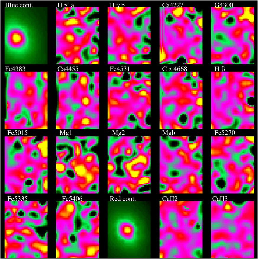
Figure 1: Maps of the most important indices in the blue and red for M 32. The maps have been scaled in a such way that pixels that are more than 2$\sigma$ fainter than the mean value of a map are black, while those more than 2$\sigma$ brighter are white. If there is a very little structure in a map, it look noisier than in a case where the dynamic range in the map is large. The size of the map is 8.2${}^{\prime\prime}\times$11^′′.

Once all these corrections were carried out line-strength maps (see Fig. 1) were obtained for the central zone of M 32 following the procedure described in P99. Note that the small structures present in the spectral index maps are mainly caused by the noise.

Next, the line indices were azimuthally averaged, and radial gradients were determined in the following way:

• We fitted five ellipses (with semi-major axes of 1.25^′′, 2.5^′′, 3.75^′′, 5.0^′′, 6.25^′′) to the isophotes of the blue and red continuum maps obtained by integrating over the whole spectral range. We used the ellipse task of the galphot package (see Jørgensen et al. 1992).

• We obtained the mean values for each spectral index in the central ellipse and in rings bound by ellipses with semi-major axis (sma) of 1.25^′′, 2.5^′′, 3.75^′′, 5.0^′′ and 6.25^′′ (with the centres corrected for differential refraction) at each wavelength. Note that the ellipses corresponding to the red continuum map were used only for the CaII triplet features.

• Each mean spectral index was plotted vs. the sma of these rings (see Fig. 2) and we determined a straight line of the form:

  $$index=(i_{0}\pm\Delta i_{0})+(m\pm\Delta m)\times r(^{\prime\prime})$$ (1)

  using a least squares fit from all the positions considered (N=5). The fits are shown in Table 2. These fits take into account the errors in the spectral index measurements (shown in Table 4), which are determined from the fibre-fibre mean dispersion (see P99 for details). The Chi-square test ($\chi^{2}=\sum_{j=1}^{N}\left(\frac{index_{j}-i_{0}-m\times r_{j}}{error_{j}}\right)^{2}$, where error_j stands for the RMS in index_j) inform us about the quality of the fit. Data indicated by T98 come from fits to longslit spectra of T98 between the center and 15^′′ (N=4 in this case).

A very important result emerges when looking at Table 2 and Fig. 2 is the fact that no gradients have been found. For none of the indices the variations in the sampled area are significant, because they are within the error bars. The absence of gradients allow us to obtain a mean value for each index in the field covered by 2D_FIS. Table 3 lists these mean values and their RMS for the first and the second night.

Table 2: Straight line fits for the indices of M32

$$\begin{array}[]{p{.08\linewidth}p{.08\linewidth}rrrrrrrr}\hline\cr\hline\cr\vskip 3.0pt plus 1.0pt minus 1.0pt\cr Index&Units&i_{0}&\Delta i_{0}&m&\Delta m&\chi^{2}&Source\\ \vskip 3.0pt plus 1.0pt minus 1.0pt\cr\hline\cr\vskip 3.0pt plus 1.0pt minus 1.0pt\cr\ CN1&mag&0.01&0.03&0.000&0.002&0.9112&T98^{\mathrm{a}}\\ \ CN2&mag&0.05&0.04&0.000&0.004&0.8747&T98\\ \ Ca4227&\AA&1.0&0.2&-0.01&0.06&0.3782&N1^{\mathrm{b}}\\ &&1.1&0.2&0.00&0.06&0.0754&N2^{\mathrm{c}}\\ &&0.9&0.5&0.06&0.05&0.5742&T98\\ \ G4300&\AA&5.3&0.3&0.09&0.08&0.4552&N1\\ &&5.5&0.3&0.00&0.08&0.3991&N2\\ &&4.9&0.3&-0.01&0.05&0.2670&T98\\ \ Fe4383&\AA&4.8&0.6&0.0&0.2&0.0313&N1\\ &&5.0&0.6&-0.1&0.2&0.0111&N2\\ &&4.9&0.7&0.01&0.07&0.2060&T98\\ \ Ca4455&\AA&1.5&0.1&0.03&0.05&0.3601&N1\\ &&1.6&0.1&0.01&0.05&0.2185&N2\\ &&1.7&0.4&0.01&0.05&0.0009&T98\\ \ Fe4531&\AA&3.3&0.3&-0.1&0.1&0.0400&N1\\ &&2.7&0.3&0.1&0.1&0.2424&N2\\ &&4.0&0.7&-0.09&0.08&1.0607&T98\\ \ C${}_{2}$4668&\AA&5.6&0.7&0.0&0.2&0.0186&N1\\ &&5.7&0.7&0.0&0.2&0.0489&N2\\ &&6&1&0.0&0.1&0.1118&T98\\ \ H$\beta$&\AA&1.9&0.2&0.02&0.05&0.2517&N1\\ &&2.0&0.2&-0.01&0.05&0.0340&N2\\ &&2.2&0.4&0.00&0.04&0.5654&T98\\ \ Fe5015&\AA&5.3&0.4&0.0&0.1&0.0845&N1\\ &&5.2&0.4&0.0&0.1&0.1414&N2\\ &&5.6&0.8&-0.02&0.09&0.0082&T98\\ \ Mg1&mag&0.082&0.007&0.000&0.002&0.1956&N1\\ &&0.074&0.007&0.001&0.002&0.1708&N2\\ &&0.07&0.01&0.001&0.001&0.2448&T98\\ \ Mg2&mag&0.193&0.008&0.002&0.003&0.9094&N1\\ &&0.191&0.008&0.002&0.003&0.1461&N2\\ &&0.19&0.01&0.001&0.002&0.1325&T98\\ \ Mgb&\AA&3.1&0.1&0.04&0.05&0.5168&N1\\ &&3.0&0.1&0.01&0.05&0.2481&N2\\ &&3.2&0.5&-0.04&0.05&0.4017&T98\\ \ Fe5270&\AA&3.0&0.2&0.05&0.07&0.0620&N1\\ &&3.0&0.2&0.00&0.07&0.0362&N2\\ &&3.1&0.2&-0.03&0.03&0.5262&T98\\ \ Fe5335&\AA&2.8&0.2&-0.05&0.08&0.0720&N1\\ &&2.5&0.2&-0.01&0.08&0.1154&N2\\ &&2.7&0.4&-0.04&0.05&0.5526&T98\\ \ Fe5406&\AA&1.8&0.2&0.03&0.06&0.1025&N1\\ &&1.8&0.2&-0.02&0.06&0.1994&N2\\ &&1.8&0.3&-0.02&0.04&0.5998&T98\\ \ Fe5709&\AA&1.1&0.3&-0.01&0.04&0.2397&T98\\ \ Fe5782&\AA&0.7&0.3&0.02&0.04&0.1213&T98\\ \ NaD&\AA&3.5&0.4&-0.04&0.05&0.4664&T98\\ \ TiO1&mag&0.04&0.01&0.000&0.001&0.6614&T98\\ \ TiO2&mag&0.06&0.01&0.000&0.001&0.3807&T98\\ \ H$\gamma$a&\AA&-3.7&0.6&-0.1&0.2&0.0038&N1\\ &&-4.0&0.6&0.0&0.2&0.0386&N2\\ \ H$\gamma$f&\AA&-0.6&0.2&-0.04&0.07&0.0728&N1\\ &&-0.6&0.2&-0.05&0.07&0.1301&N2\\ \ Ca1&\AA&1.9&0.6&-0.1&0.2&0.1006&N1\\ &&1.9&0.6&0.0&0.2&0.0518&N2\\ \ Ca2&\AA&4.0&0.6&0.0&0.2&0.0580&N1\\ &&4.4&0.6&0.0&0.2&0.0748&N2\\ \ Ca3&\AA&3.4&0.6&0.0&0.2&0.0415&N1\\ &&3.1&0.6&0.2&0.2&0.2717&N2\\ \ Ca2+3&\AA&7.4&0.8&-0.1&0.3&0.0388&N1\\ &&7.6&0.8&0.2&0.3&0.3022&N2\\ \vskip 3.0pt plus 1.0pt minus 1.0pt\cr\hline\cr\end{array}$$

Table 2: Straight line fits - continued

$$\begin{array}[]{p{.08\linewidth}p{.08\linewidth}rrrrrrrr}\hline\cr\hline\cr\vskip 3.0pt plus 1.0pt minus 1.0pt\cr Index&Units&i_{0}&\Delta i_{0}&m&\Delta m&\chi^{2}&Source\\ \vskip 3.0pt plus 1.0pt minus 1.0pt\cr\hline\cr\vskip 3.0pt plus 1.0pt minus 1.0pt\cr\ CaAZ1&\AA&1.7&0.3&-0.03&0.09&0.2363&N1\\ &&1.6&0.3&-0.03&0.09&0.1611&N2\\ \ CaAZ2&\AA&3.6&0.3&-0.03&0.01&0.2362&N1\\ &&3.8&0.3&-0.11&0.01&0.4563&N2\\ \ CaAZ3&\AA&2.9&0.3&0.01&0.09&0.2146&N1\\ &&2.9&0.3&0.02&0.09&0.4930&N2\\ \ CaAD1&\AA&3.7&0.3&0.0&0.1&0.1379&N1\\ &&3.9&0.3&0.0&0.1&0.2184&N2\\ \ CaAD2&\AA&3.0&0.3&0.0&0.1&0.2490&N1\\ &&2.9&0.3&0.0&0.1&0.4718&N2\\ \ CaTP1&\AA&1.8&0.3&0.0&0.1&0.1144&N1\\ &&1.9&0.3&0.0&0.1&0.0592&N2\\ \ CaTP2&\AA&3.9&0.3&0.0&0.1&0.0794&N1\\ &&4.2&0.3&-0.1&0.1&0.3166&N2\\ \ CaTP3&\AA&2.7&0.3&0.0&0.1&0.2064&N1\\ &&2.6&0.3&0.1&0.1&0.1931&N2\\ \vskip 3.0pt plus 1.0pt minus 1.0pt\cr\hline\cr\end{array}$$

• long-slit between 0^′′ and 15^′′ of distance from the centre (T98).

• 2D$\_$FIS data from the 15 February, Night 1.

• 2D$\_$FIS data from the 16 February, Night 2.

Table 3: Observed average spectral indices

$$\begin{array}[]{p{.07\linewidth}p{.07\linewidth}rrrrrr}\hline\cr\hline\cr\vskip 3.0pt plus 1.0pt minus 1.0pt\cr{}&{}&\lx@intercol\hfil Night1\hfil\lx@intercol&\lx@intercol\hfil Night2\hfil\lx@intercol\\ Index&Units&mean&error&mean&error\\ \vskip 3.0pt plus 1.0pt minus 1.0pt\cr\hline\cr\vskip 3.0pt plus 1.0pt minus 1.0pt\cr H$\gamma$a&\AA&-4.1&0.5&-3.9&0.5\\ H$\gamma$f&\AA&-0.7&0.3&-0.7&0.3\\ Ca4227&\AA&1.0&0.2&1.0&0.2\\ G4300&\AA&5.7&0.5&5.5&0.5\\ Fe4383&\AA&5.0&0.6&4.7&0.6\\ Ca4455&\AA&1.5&0.3&1.7&0.2\\ Fe4531&\AA&3.0&0.5&2.9&0.8\\ C${}_{2}$4668&\AA&5.7&0.8&5.8&0.6\\ H$\beta$&\AA&2.0&0.3&2.0&0.2\\ Fe5015&\AA&5.2&0.5&5.1&0.5\\ Mg1&mag&0.08&0.01&0.08&0.01\\ Mg2&mag&0.20&0.01&0.20&0.01\\ Mgb&\AA&3.2&0.3&3.0&0.2\\ Fe5270&\AA&3.2&0.3&3.0&0.2\\ Fe5335&\AA&2.6&0.3&2.5&0.2\\ Fe5406&\AA&1.9&0.3&1.8&0.3\\ CaII2&\AA&3.8&0.6&3.8&0.6\\ CaII3&\AA&3.4&0.7&3.4&0.7\\ \vskip 3.0pt plus 1.0pt minus 1.0pt\cr\hline\cr\end{array}$$

2.3 Comparison with previous results

Fig. 2 shows our index measurements compared to those of T98, showing very good agreement. Note that despite the fact that their results were achieved with long-slit spectroscopy we can compare with our 2D_FIS field, since no gradients were found and therefore the indices do not depend on the slit position. The only significant difference is obtained for the G band (which is $\sim$15 $\%$ or 1.8 $\sigma$ larger in our case).

3 The stellar population analysis

3.1 Observational constrains

The next step was to analyze the stellar populations. We decided to add to the data, in addition to the line strengths, also a set of optical and near-infrared colours obtained by Peletier (1993), mainly to constrain the shape of the continuum and to include spectral indices at other different spectral regions for which different stars contribute in a different way. We averaged the colours in the same region of the galaxy, and corrected for Galactic extinction using the DIRBE-maps analyzed by Schlegel et al. (1998), and the Galactic extinction law given by Rieke & Lebofsky (1985). In Table 4, the colours that we used are given together with the line indices. We used various age indicators, such as H$\beta$ (W94), and H$\gamma$A and H$\gamma$F (Worthey & Ottaviani 1997). These indices when plotted against strong metallicity indicators like the iron or magnesium dominated lines are able to constrain reasonably well both the age and the metallicity of the stellar population (e.g., W94; Vazdekis et al. 1997). When these metallicity indicators are plotted against each other they show that giant ellipticals have [Mg/Fe]$>$0.0 (e.g., Peletier 1989; Worthey et al. 1992).We also observed the Ca4227 index, which was found to be much lower than expected in a number of early-type galaxies by Vazdekis et al. (1997) and P99. Index-index diagrams allow us to note the very strong CN absorption of the metal-rich globular clusters (e.g.: Rose 1994; Vazdekis 1999a). One of the metal indicators is C₂4668, shown by Tripicco & Bell (1995) to be an excellent indicator for the global metallicity. This index was found very useful to analyze the Fornax early-type galaxies (Kuntschner & Davies 1998). We have also included a number of indicators which can help in constraining the dwarf/giant ratios and the IMF such as the CaII triplet features (Díaz et al. 1989) and TiO₁ (see V96 (Table 2) and Vazdekis et al. 1997 (Fig. 10)). Vazdekis (1999b) showed that no powerful IMF indicators are present in the range $\lambda\lambda$ (4000-5500Å) (Mg₁ being the most sensitive of these).

3.2 Models

For the stellar population analysis we decided to use the models of W94 and V96. These two models predict single-age single-metallicity stellar populations for intermediate and old stellar populations. The models of V96 have recently been updated by implementing the new metallic dependent empirical relations of Alonso et al. (1999) for giants with temperatures larger than $\sim$3500 K for all metallicities, and by applying a semi-empirical approach for the coolest dwarfs and giants on the basis of the empirical color-T_eff relations of Lejeune et al. (1997) and Lejeune et al. (1998) for solar metallicity, and the stellar model atmospheres of Hauschildt et al. (1999). These models are (see http://star-www.dur.ac.uk/$\sim$vazdekis for the latest version) now more accurate and cover a larger range of ages and metallicities. The differences with V96 in general are small, especially for solar metallicity; only the IR colors vary slightly. W94 uses a Salpeter (1955) IMF, while V96 provides models with 2 different IMFs: the Unimodal, which is a power-law, with the slope as a free parameter (where 1.3 corresponds to Salpeter), and a Bimodal IMF, where the number of stars of mass $<$0.6 M_⊙ has been truncated. These models all include the optical spectral indices of the Lick/IDS system. The V96 model also predicts the CaII triplet features on the system of Díaz et al. (1989).

3.3 The fits

In Figure 3 and 4 various index-index and colour-index diagrams together with the model predictions of V96 (for a bimodal IMF with slopes 1.35 and 2.35) are shown. These plots show that most of the observed colours and indices indicate that the average metallicity of the galaxy lies between Z=0.008 and Z=0.05, and is very close to Z=0.02. In addition, the spectral indices observed are between the isolines corresponding to ages of 2.5 and 6.3 Gyrs. It is important to note that these plots do not show any strong discrepancies between models and observations. This allows us to conclude that element ratios in this galaxy do not strongly differ from those in the solar neighbourhood. Although this might seem surprising, since giant ellipticals generally have Mg/Fe abundance ratios that are larger than solar (e.g. Peletier 1989, Worthey et al. 1992, Vazdekis et al. 1997, Trager et al. 2000), it is in agreement with previous results, since the Mg/Fe overabundance seems to correlate with the luminosity of a galaxy, in a way that faint ellipticals have solar abundance ratios (e.g. Worthey 1998, Trager et al. 2000).

To be able to obtain a more detailed fit and to constrain the number of possible solutions we used all the information provided by our large set of indices and colors via the Merit Function MF^J(A,Z), which, for each model J, depends on the age (A) and the metallicity (Z):

$$MF^{J}(A,Z)=\frac{\sum_{i=1}^{n}~{}W_{i}~{}\times~{}\left(\frac{O_{i}-M_{i}^{J}}{E_{i}}\right)^{2}}{\sum_{i=1}^{n}~{}W_{i}},$$ (2)

where n is the number of observed spectral indices, O_i is the observed value of the index i , M${}_{i}^{J}$(A,Z) is the synthetic value for this color/index predicted by model J, and E_i is its corresponding observational error. Finally, W_i represents its relative weight. Following the fact that we have not found any significant departure from the solar neighbourhood element ratio trends we have chosen to assign a weight of $1$ to all the indices. This approach differs from that used in Vazdekis et al. (1997) and P99 for fitting a sample of considerably more luminous galaxies, which showed appreciable differences in their element ratios. These authors demonstrated that the inferred age/metallicity depends on the relative weights of the colours and indices (see also Vazdekis 1999a, Kuntschner 2000). For example, they found that the analysis on the basis of the Fe dominated indices yielded a lower metallicity than the one obtained on the basis of the Mg dominated features. Fortunately, the solution for M 32 is to a large extend free from these effects and the models (which are based on solar element ratios) seem fully appropriate, making it possible to use the information provided by the whole set of indices.

We built up contour plots of MF^J(A,Z) for each J-model using an interpolation program based on the Renka-Cline method described in the Numerical Recipes (Press et al. 1992). We recall that this method warrants that the reconstructed surface is continuous with continuous first derivatives. The minimum of this surface was then determinated using the downhill simplex method carried out by the AMOEBA subroutine of the Numerical Recipes. Therefore, for each J-model we could determine the most probable solution (for the metallicity and the age) where MF^J(A,Z) yield the lowest values.

We used various types of models: i) models of V96 with a unimodal, Salpeter IMF with slope x=1.35 (M1), ii) models of V96 with unimodal IMF and x=2.35 (M2), iii) models with bimodal (as defined in V96) IMF with x=1.35 (M3), iv) models with bimodal IMF with x=2.35 (M4), and v) W94 models with a Salpeter IMF (M5).

Table 4: Observed and modeled spectral indices

$$\begin{array}[]{p{.08\linewidth}p{.07\linewidth}cccccccccc}\hline\cr\hline\cr\vskip 3.0pt plus 1.0pt minus 1.0pt\cr\ Index&Units&MeanObs&Error&Source&Obs-M_{1}&Obs-M_{2}&Obs-M_{3}&Obs-M_{4}&Obs-M_{5}\\ \vskip 3.0pt plus 1.0pt minus 1.0pt\cr\hline\cr U-V&mag&1.28&0.05&(P93)^{\mathrm{a}}&-0.07&-0.06&-0.06&-0.04&0.03\\ B-V&mag&0.85&0.05&(P93)&-0.04&-0.05&-0.04&-0.03&-0.07\\ V-R&mag&0.52&0.05&(P93)&-0.03&-0.05&-0.03&-0.03&-0.04\\ V-I&mag&1.13&0.05&(P93)&-0.02&-0.09&-0.01&-0.02&-0.05\\ V-J&mag&2.20&0.05&(P93)&0.00&-0.09&0.02&0.04&0.03\\ V-K&mag&3.05&0.05&(P93)&-0.12&-0.18&-0.11&-0.06&-0.01\\ H$\gamma$a&\AA&-4.1&0.5&(D15)^{\mathrm{b}}&0.5&0.3&0.5&0.4&-0.3\\ H$\gamma$f&\AA&-0.7&0.3&(D15)&-0.1&-0.1&-0.1&-0.1&-0.5\\ CN1&mag&0.01&0.02&(T98)^{\mathrm{c}}&-0.01&0.01&-0.01&0.01&0.01\\ CN2&mag&0.05&0.02&(T98)&0.00&0.01&0.00&0.01&0.02\\ Ca4227&\AA&1.0&0.2&(D15)&-0.3&-0.4&-0.3&-0.3&-0.1\\ G4300&\AA&5.7&0.5&(D15)&0.8&0.9&0.8&0.9&1.2\\ Fe4383&\AA&5.0&0.5&(D15)&0.2&0.3&0.2&0.3&0.5\\ Ca4455&\AA&1.5&0.3&(D15)&0.0&0.0&0.0&0.0&0.0\\ Fe4531&\AA&3.0&0.5&(D15)&-0.3&-0.3&-0.2&-0.3&-0.2\\ C${}_{2}$4668&\AA&5.7&0.8&(D15)&0.9&1.2&0.9&1.2&1.2\\ H$\beta$&\AA&2.0&0.3&(D15)&0.0&0.1&0.0&0.0&-0.1\\ Fe5015&\AA&5.2&0.5&(D15)&-0.2&0.0&-0.2&-0.1&-0.1\\ Mg1&mag&0.08&0.02&(D15)&-0.01&-0.01&-0.01&-0.01&0.00\\ Mg2&mag&0.20&0.01&(D15)&-0.02&-0.03&-0.02&-0.02&-0.01\\ Mgb&\AA&3.2&0.3&(D15)&-0.2&-0.3&-0.2&-0.2&0.0\\ Fe5270&\AA&3.2&0.3&(D15)&0.4&0.4&0.4&0.4&0.4\\ Fe5335&\AA&2.6&0.3&(D15)&0.1&0.1&0.1&0.1&0.1\\ Fe5406&\AA&1.9&0.3&(D15)&0.3&0.3&0.3&0.3&0.3\\ Fe5709&\AA&1.1&0.2&(T98)&0.1&0.2&0.1&0.2&0.2\\ Fe5782&\AA&0.8&0.2&(T98)&0.0&0.0&0.0&0.0&0.0\\ NaD&\AA&3.4&0.2&(T98)&0.4&-0.1&0.5&0.2&0.6\\ TiO1&mag&0.037&0.007&(T98)&-0.003&-0.010&-0.003&-0.003&-0.010\\ TiO2&mag&0.061&0.006&(T98)&-0.001&-0.014&0.001&0.000&-0.016\\ CaII+&\AA&7.2&0.8&(D15)&-1.2&-0.9&-1.2&-1.0&...\\ \vskip 3.0pt plus 1.0pt minus 1.0pt\cr\hline\cr\end{array}$$

• Simulated long-slit data of a region 2^′′ from the centre (Peletier, 1993).

• 2D$\_$FIS data corresponding to the mean values in the 9^′′$\times$12^′′ central region obtained on 15 February.

• long-slit data of the centre (T98).

Table 5: Ages and metallicities for M32

$$\begin{array}[]{p{.08\linewidth}cccc}\hline\cr\hline\cr\vskip 3.0pt plus 1.0pt minus 1.0pt\cr Model&Z&Age&MF^{J}(A,Z)\\ &&(Gyr)&\\ \vskip 3.0pt plus 1.0pt minus 1.0pt\cr\hline\cr M1&0.02&4.0&1.0\\ M2&0.02&4.0&1.8\\ M3&0.02&4.0&1.0\\ M4&0.02&4.0&0.8\\ M5&0.019&5.0&1.4\\ \vskip 3.0pt plus 1.0pt minus 1.0pt\cr\hline\cr\end{array}$$

4 Results

4.1 A single age-metallicity solution

Figs. 5, 6 and 7 show contour plots of the MF as a function of metallicity (Z) and age (A) for the different models. MF values lower than 1 represent fits which are fully acceptable within the error bars of the observed data. However, to prevent the exclusion of any possible solution we consider a fit acceptable when MF value is lower than 1.5. In Table 5 we tabulate the best fits for the age and the metallicity and the corresponding MF^J(A,Z) values achieved with each model. We see that all the models predict a similar age ($\sim$4 Gyr) and a solar-like metallicity (W94 models provide a slightly larger age $\sim$5 Gyr). The contours of the MF plots also show that fits with ages in the range (3-6 Gyr) and metallicities in the range (0.015-0.025) cannot be discarded. It is worth recalling that the contours of the MF are indicating the well known age-metallicity degeneracy: older ages require lower metallicities and viceversa. However, the contours are more elongated toward the older ages than to the younger ones because the indices and colors of the stellar populations evolve more slowly for larger ages (e.g., W94; V96). It is also interesting to see that these contours are more elongated for the W94 models. The MF plots and Table 5 show some differences between the models. In fact, M2 does not provide any reasonable fit to the observed indices and colors. Overall, V96’s models with an unimodal IMF and slope x=1.35 (M1) or the models with bimodal IMFs (M3,M4) provide the best fits. The best solution is reached when using M4 (MF=0.8). Table 4 lists the differences between observations and models (M1, M2, M3, M4 and M5) for colors and indices corresponding to each solution (A,Z) shown in Table 5. In this table MF^J(A,Z) for each solution (A,Z) is also listed.

4.2 Giants versus dwarfs

In Table 6 we tabulate the relative contribution of the dwarfs to several spectral bands from ultraviolet to infrared. We do this for SSPs of 4 Gyr and solar metallicity, using V96’s models. We see that the dwarfs contribute $\sim$80% of the total light in the U-band, while in K the giants dominate the total light with a very similar proportion. In V, the dwarfs and giants contribute $\sim$50% each.

Table 6: Contribution of the dwarfs (in %) to the total light for a SSP of 4 Gyr and Z=0.02

$$\begin{array}[]{p{.07\linewidth}ccccccccc}\hline\cr\hline\cr\vskip 3.0pt plus 1.0pt minus 1.0pt\cr Model&U&B&V&R&I&J&H&K\\ \vskip 3.0pt plus 1.0pt minus 1.0pt\cr\hline\cr M1&80.1&61.7&49.0&42.8&35.2&22.4&16.7&14.6\\ M2&83.1&67.2&56.6&52.3&48.9&40.3&34.1&32.3\\ M3&80.1&61.7&49.2&43.1&36.0&23.8&18.0&15.9\\ M4&83.0&66.7&55.4&50.1&43.6&31.0&24.7&22.2\\ \vskip 3.0pt plus 1.0pt minus 1.0pt\cr\hline\cr\end{array}$$

Table 6 suggests that the changes to colors as a result of varying the IMF are largest for the largest wavelength range between the 2 bands constituting this colour. This means that the effect on a color like $V-K$ is much larger than e.g. $V-R$ (in agreement with Vazdekis 1999b). It should be noted, however, that the effects of changing the IMF, for the bimodal case, are much smaller than for the unimodal case, since in the bimodal case there is a lower number of stars with masses smaller than 0.6 M_⊙, the stars which are red enough to contribute substantially to the $V-K$ color. The table also shows that the relative contribution of dwarfs and giants does not vary very much from model to model, except for model M2, which is unimodal, with x=2.35. Even here significant differences are only seen for the reddest bands. In fact, this model is not able to fit the galaxy because it provides near-IR colors (e.g., $V-K$) that are too red (see Table 4). Note, however, that the optical line-strengths of this model (with the exception of the reddest ones, like the TiO-bands) are not very different from those of the models M1, M3 and M4. M1, M3 and M4 give similar fits, although model M4, which has a slightly larger contribution of dwarfs than M1 and M3, provides a somewhat lower MF value.

5 Discussion

5.1 Gradients

The optical and infrared photometry shows no evidence for the presence of gradients in the colors (Peletier 1993, Lauer 1998). The V-I and U-V images ofthe HST (Lauer, 1998) are essentially flat, without any sign of structure (dust, inner disk, etc.). Ultraviolet colours show strong gradients, e.g., in the (152 – 249) colour (O’Connell et al. 1992) and the m₁₅₀₀ – B colour (Ohl et al. 1998), in the sense that M32 is redder in the centre. Its behaviour is opposite to all other objects studied by these authors, and also therefore not well understood. It is not in conflict with the optical data, since a few hot stars can affect the UV bands without noticeably altering the optical colours. A possible explanation could be that the m₁₅₀₀ – B gradient is caused by a slightly older centre.

Concerning the line-strength gradients, González (1993) pointed out that various indices show relatively small, but monotonically decreasing profiles, particularly H$\beta$ and Fe5270. Davidge (1991) detected a very small gradient in the inner 5 arcsec. Hardy et al. (1994) noted that the line indices are smaller in the outer parts. However, our 2D_FIS data do not show any significant gradient for the central 9${}^{\prime\prime}\times$12^′′ region of this galaxy. Also, the data of T98 rule out any variation of the line strength profiles in the inner 15 arcsec. The H$\beta$ gradient of González (1993) suggests that the galaxy is younger in the centre. However, to obtain a constant color or Mg₂ profile the galaxy needs to be at the same time more metal-rich towards the centre, so that both effects cancel each other out. In the inner areas discussed here these gradients are negligible. Measurable age- or metallicity gradients could be present when going to larger radii, but this is outside the scope of this paper.

5.2 Age and Metallicity

The large number of indices and colors used in this work allowed us to constrain the age and the metallicity for this galaxy, although the contours of the MF plots still show some of the effects of the age-metallicity degeneracy. The best fits suggest an age of 4 Gyr and a solar-like metallicity. This result is in agreement with previous results (O’Connell 1980; Burstein et al. 1984; Rose 1985,1994; Faber et al. 1992; Hardy et al. 1994; Dorman et al. 1995; Vazdekis & Arimoto 1999). The spectrophotometric study of O’Connell (1980) suggested that the turnoff stars should be close to F8. Burstein et al. (1984) also conclude that turnoff stars with spectral types F6–F9 are needed to make H$\beta$ strong enough to fit the value for M 32. In that paper the authors rule out models with many blue stragglers or a strong BHB. Dorman et al. (1995) exclude the presence of a representative contribution of RHB stars and conclude that M 32 has an intermediate age and a solar-like metallicity. Boulade et al. (1988) reach the same conclusion from the spectral range between $\lambda\lambda$3200 and 3900 Å . Rose (1985, 1994) on the basis of the spectral range around $\lambda$4000Å concluded that this galaxy has no significant contribution from a RHB population, and has a more metal-rich main-sequence turnoff and a larger hot star contribution than is inferred to be present in 47 Tuc. More recently Rose & Deng (1999) reach the same conclusions on the basis of an analysis of IUE mid-ultraviolet low resolution spectra. Our result is in full agreement with that of Vazdekis & Arimoto (1999), who predicted an age of 4 Gyr and solar-like metallicity from a very good fit to the blue spectrum of this galaxy, using a new spectroscopic age indicator.

There are, however, other authors who suggest a larger age. Jones & Worthey (1995) obtained 7 Gyr based on their H$\gamma_{HR}$ index. Vazdekis & Arimoto (1999) attributed this difference to the fact that W94 model makes use of isochrones which are slightly hotter than those of V96’s model and to the fact that H$\gamma_{HR}$ is very sensitive to the resolution and to the velocity dispersion effect. A relatively recent HST analysis resolving M 32 into individual stars (Grillmair et al. 1996) suggests a wide metallicity spread (but smaller than expected from the simple model) and the presence of SMR stars on the basis of the observed color spread of AGB and RGB stars. Also, their color-magnitude diagrams do not indicate the presence of bright AGB stars as claimed by Freedman et al. (1992). Although they do not distinguish between age and metallicity using colors, they infer an age of 8.5 Gyr (for at least a 50% of its stellar populations) and a metallicity [Fe/H]=-0.25 (Z=0.014). Although their solution for the age and metallicity is inferred from the indices of T98 using W94 models, our analysis (see model M5 in Table 5) is in disagreement with their conclusion. In our opinion their data suffers from the age-metallicity degeneracy, and resolving individual stars does not help in solving this problem.

5.3 Unique solution

Our data have been successfully fitted with a single-age, single-metallicity stellar population as has been done by other authors (e.g.: Vazdekis & Arimoto 1999). However, it has been suggested that M 32 contains 2 stellar populations, an underlying old stellar population, together with a second stellar population of younger stars (see, e.g., O’Connell 1980). We have tested this idea, and investigated what the best solution is, for a linear combination consisting of an old population of 17 Gyr and Z=0.02, and a young population with Z=0.02 and variable age between 1 and 5 Gyr, using model M4. The results are given in Table 7. As expected, the relative contribution of the young stellar population decreases when considering ages closer to 1 Gyr. We find that the minimum MF is obtained for a combined stellar population of 3.2 Gyrs and 17 Gyrs (82% and 18%, respectively) but all the tabulated combinations are acceptable, because the MF$<$1.5. To really constrain the 2-population model, more indices in the near and far UV are needed.

Table 7: Percentage of the young stars with ages between 1-4 Gyrs for a combined stellar population formed by these stars and others with 17 Gyrs (fixed Z=0.02) according to model M4. The Merit Function values are also tabulated.

$$\begin{array}[]{p{.15\linewidth}ccccccccc}\hline\cr\hline\cr\vskip 3.0pt plus 1.0pt minus 1.0pt\cr Age (Gyrs)&1.0&1.6&2.0&2.5&3.2&4.0&5.0\\ \vskip 3.0pt plus 1.0pt minus 1.0pt\cr\hline\cr\% Young pop.&35&50&58&69&82&100.&100.\\ MF&1.32&1.12&1.02&0.91&0.88&0.94&1.34\\ \vskip 3.0pt plus 1.0pt minus 1.0pt\cr\hline\cr\end{array}$$

5.4 Abundance Ratios

Our 2D_FIS data do not show any significant departure from solar-like element ratios. However, we have found a number of indices which slightly differ from the models, such as C₂4668, which is slightly larger than the predicted values. This feature has been claimed by Worthey (1994) as a strong metallicity indicator, and Tripicco & Bell (1995) showed that this is an indicator of the global metallicity. Kuntschner & Davies (1998) found that the H$\gamma$A-C₂4668 diagram is very useful for studying the age and the metallicity. More recently Kuntschner (2000) suggested that this index seems to be too strong compared to Fe for galaxies for which the C₂4668 line-strength is larger than $\sim$6 Å. We obtain 5.7 Å while a slightly higher value is tabulated in T98. However, we should be aware that this index has a wide central bandpass (86.25 Å) and therefore could be affected by systematic errors. Note for example the large transformation factors given in Table 3 of P99. The G band is significantly larger than the model predictions but this difference is not as large if we consider the value of T98. In fact, we do not exclude that some systematic error in this spectral range could be affecting our data here, as well. The CaII triplet feature is low compared with the solar metallicity model predictions. It is surprising that our value (7.2 Å) is very similar to the mean value of the nuclei of normal galaxies (7.1 Å, Terlevich et al. 1990) and also the three galaxies in P99 that were observed with the same instrument, even though M 32 is much less massive, and other indices are generally much smaller. This indicates that the Ca triplet could be a great giant/dwarf discriminator. However, we point out that the model predictions for this index are much less accurate than the others because of the lack of completeness of the library of Díaz et al. (1989). A new extensive stellar spectral library covering this feature will be soon available (Cenarro et al. 2000, in preparation).

Our results provide reasonably good fits to the other absorption line-strengths. It is interesting to note that we obtain an excellent fit to the strength of H$\beta$ while O’Connell (1980) found that it was 3$\sigma$ too weak compared to his models. The difference is probably due to the fact that the models are now better than before.

For most of the indices the obtained fits provide line-strengths that fall within the error bars of the measurements (i.e., MF$\sim$1). However, there are a number of indices which deviate slightly from the predicted values, in a systematic way. For example, for the CaII triplet features the observed values are lower than the model predictions for solar metallicity (see also P99). The predicted values, however, might not be very accurate (see the above discussion). The Ca4227 line is also slightly lower than the model predictions, but, on the other hand, the value provided by T98 is slightly higher than ours. We also see that the G band it is 1.8 $\sigma$ larger than in the models. This difference, however, is reduced if we use instead the G-band value given by T98, which is considerably lower. This suggests that our G band measurement could be affected by fringing in the 2D_FIS spectra. Concerning the Mg/Fe relation we see that all the residuals for these lines are within the error bars. Note, however, that while the residuals of the Mg lines are negative most of the residuals of the Fe features are positive, except for indices Fe4531 and Fe5015.

5.5 Dwarfs/Giants

The best fits obtained here suggest that the dwarfs contribute to the total light $\sim$80-83% in the U filter, $\sim$61-67% in B, $\sim$49-56% in V, $\sim$43-50% in R, $\sim$35-44% in I, $\sim$22-31% in J, $\sim$17-25% in H and $\sim$14-23% in K. These values have been obtained on the basis of models M1, M3 and M4 (i.e., V96 models with unimodal IMF with slope 1.3 and bimodal models with slope 1.3 and 2.3). Rose (1994) used various diagrams such as SrII$\lambda$4077/FeI$\lambda$4045 versus H$\delta$/FeI$\lambda$4045 to conclude a dwarfs/giants relation of 0.65:0.35 which is in perfect agreement with our estimate for the B filter. The luminosity-weighted mean surface gravity for M 32 at 3500 Å indicates that the giant branch contributes slightly less than 30% of the light at 4000 Å (Boulade et al. 1988). This is in agreement with our estimation in the filter U.

Concerning the IMF slope, CO (2.3$\mu$m) data of early-type galaxies (not including M 32) with -19$\leq M_{v}\leq$-23 could be adequately fitted by models with IMF slope x=1.35 (Aaronson 1978). He gave an upper limit for x=2.25. Here we have shown that the main changes introduced by changes in the IMF should be found for the spectral indices and colors centred at the longest wavelengths. In fact, we see significant differences in, e.g., the V-K color or the CaII features. However, the present model and observational uncertainties do not allow us to constrain the IMF more strongly.

6 Conclusions

We have obtained Integral Field Spectroscopy of the 9${}^{\prime\prime}\times$12^′′ circumnuclear region of M32. From these spectra, we have applied a stellar population analysis using 30 spectral indices and colours. Our main conclusions are:

1. None of the spectral index maps show significant variations in the sampled area. This result is in agreement with long-slit spectroscopy in the literature (T98).

2. From the population synthesis models of V96 and W94 we find that the best-fitting models have an age of 4 Gyrs and a solar-like metallicity for the nuclear region of M 32. We have found that the element abundance ratios are generally the same as in the sun. Models with a Salpeter IMF with a slope of 2.35 or larger are excluded. Although our data can be successfully interpreted with a single age-metallicity stellar population, it is also possible to fit them with a linear combination of an old stellar population of 17 Gyr and Z=0.02 and a young stellar population with age 1-5 Gyr.

3. Our best fits using the model of V96 suggest that the dwarfs contribute to the total light $\sim$80-83% in the U filter, $\sim$61-67% in B, $\sim$49-56% in V, $\sim$43-50% in R, $\sim$35-44% in I, $\sim$22-31% in J, $\sim$17-25% in H and $\sim$14-23% in K.

Figure Captions

Figure 2: Spectral indices as a function of radius for 2D_FIS data (open circles) and data of T98 (filled circles).

Figure 3: Spectral index-index diagrams. Data from here (open circles) and from T98 (filled circles) are plotted. The bimodal models with IMF slope of 1.35 (continuous line) and 2.35 (dashed line) of Vazdekis et al. (1996) are plotted for metallicites Z=0.008 (thin line), 0.02 (intermediate line) and 0.05 (thick line). Ages correspond to 1.0, 2.5, 6.3 and 17.4 Gyrs, respectively, from the thinnest to thickest dotted line.

Figure 4: For lines and symbols see Fig.  3.

Figure 5: Contours of the Merit Function for unimodal models with IMF slope x=1.35 (top) and x=2.35 (bottom).

Figure 6: Contours of the Merit Function for bimodal models with IMF slope x=1.35 (top) and x=2.35 (bottom).

Figure 7: Contours of the Merit Function for the Worthey model.

References

- [] Aaronson M., Cohen J. G., Mould J. & Malkan M. 1978, ApJ, 223, 824
- [] Allen C. W. 1973, Astrophysical Quantities (3rd Ed.; London: Athlone)
- [] Alonso A., Arribas S. & Martínez-Roger C. 1999 A&AS, 139, 335
- [] Arimoto N. & Yoshii Y. 1986 A&A, 164, 260
- [] Arribas S. & Mediavilla E. 2000, in “Imaging the Universe in Three Dimensions: Astrophysics with Advanced Multi-Wavelength Imaging Devices”, to appear in ASP Conference Series
- [] Arribas S., Mediavilla E., García-Lorenzo B., del Burgo C. & Fuensalidad J. J., 1999, A&AS, 136, 189
- [] Bica E., Alloin D. & Schmidt A. A. 1990, A&A 228, 23
- [] Bertelli G., Bressan A., Chiosi C., Fagotto F. & Nasi E. 1994, A&AS, 106, 275
- [] Bertola F., Capaccioli M. & Oke J. B. 1982, ApJ, 254, 494
- [] Boulade O., Rose J. A., Vigroux L. 1988, AJ, 96, 1319
- [] Burstein D., Bertola F., Buson L. M., Faber S. M. & Lauer T. R. 1988, ApJ, 328, 400
- [] Burstein D., Faber S. M., Gaskell C. M. & Krumm N. 1984, ApJ, 287, 586
- [] Burstein D. & Heiles C. 1978, ApJ, 225, 40
- [] Cenarro J. et al. 2000, in preparation
- [] Davidge T. J. 1991, AJ, 101, 884
- [] Davidge T. J. & Jones J. H. 1992, AJ 104, 1365
- [] Díaz A. I., Terlevich E. & Terlevich R. 1989, MNRAS, 239, 325
- [] Dorman B., O’Connell R. W., Rood R. T. 1995, ApJ, 442, 105
- [] Faber S. M. 1972, A&A, 20, 361
- [] Faber S. M., Friel E. D., Burstein D. & Gaskell C. M. 1985, ApJS, 57, 711
- [] Faber S. M., Worthey G. & Gonzales J. J. 1992, in The Stellar Populations of Galaxies. Proceedings of the IAU Symposium no. 149, ed. B. Barbuy & A. Renzini
- [] Freedman W. L. 1992, AJ 104, 1349
- [] García A., Rasilla J. L., Arribas S., & Mediavilla E. 1994, in Instrumentation in Astronomy VIII, SPIE Vol. 2198, ed. D. L. Crawford & C. R. Craine (Hawaii: SPIE), 75
- [] González J. J. 1993, PhD. Thesis, University of Lick, Santa Cruz, California
- [] Gorgas J., Faber S. M., Burstein D., González J. J., Courteau S. & Prosser C. 1993, ApJS, 86, 153
- [] Grillmair C. J., Lauer T. R., Worthey G., Faber S. M., Freedman W. L., Madore B. F., Ajhar E. A., Baum W. A., Holtzman J. A., Lynds C. R. O’Neil E. J. Jr., Stetson P. B. 1996, AJ, 112, 1975
- [] Hauschildt P. H., Allard F., Ferguson J., Baron E. & Alexander, D. R. 1999, ApJ, 525, 871
- [] Hauschildt P. H., Allard F. & Baron E. 1999, ApJ, 512, 377
- [] Jones L. A., Worthey G. 1995, ApJL, 446, 31
- [] Jørgensen I., Franx M., Kjaergaard P. 1992, A&AS, 95, 489
- [] Kuntschner, H., 2000, MNRAS, accepted
- [] Kuntschner H. & Davies R. L. 1998, MNRAS, 295, 29
- [] Hauschildt P. H., Allard F. & Baron E. 1999, ApJ, 512, 377
- [] Hardy E., Couture J., Couture C. & Gilles J. 1994, AJ 107, 195
- [] Lauer T. R., Faber S. M., Ajhar E. A., Grillmair C. J. & Scowen P. A. 1998, AJ, 116, 2263
- [] Lejeune T., Cuisinier F., Buser R. 1998, A&AS, 130, 65
- [] O’Connell R. W. 1980, ApJ, 236, 430
- [] O’Connell R. W. 1976, ApJ, 206, 370
- [] O’Connell R. W. Bohlin R. C., Collins N. R., Cornett R. H., Hill J. K., Hill R. S., Landsman W. B., Roberts M. S., Smith A. M. & Stecher T. P. 1992 ApJL, 395, 45
- [] Ohl R. G., O’Connell R. W., Bohlin R. C., Collins N. R., Dorman B. Fanelli M. N., Neff S. G., Roberts M. S., Smith A. M. & Stecher T. P. 1998, ApJL, 505, 11
- [] Peletier R. F. & Valentijn E. A. 1989, Ap&SS, 156, 127
- [] Peletier R. F. 1993, A&A, 271, 51
- [] Peletier R. F., Vazdekis A., Arribas S., del Burgo C., García-Lorenzo B., Gutierrez C., Mediavilla E. & Prada F. 1999, MNRAS, 310, 863 (P99)
- [] Press W. H., Teukolsky S. A., Vetterling W. T. & Flannery B. P. 1992, Numerical recipes in FORTRAN. The art of scientific computing, Cambridge: University Press, 2nd ed.
- [] Rieke G. H. & Lebofsky M. J. 1985, ApJ, 288, 618
- [] Rose J. A. 1985, AJ, 90, 1927
- [] Rose J. A. 1994, AJ, 107, 206
- [] Rose J. A. & Deng S. 1999, AJ, 117, 2213
- [] Salpeter E. E. 1955, ApJ, 121, 161
- [] Schlegel D. J., Finkbeiner D. P. & Davis M. 1998, AJ, 115, 525
- [] Spinrad & Taylor 1969, ApJ, 157, 1279
- [] Tantalo R., Chiosi C. & Bressan A. 1998, A&A, 333, 419
- [] Terlevich E., Díaz A. I. & Terlevich R. 1990, MNRAS, 242, 271
- [] Tinsley B. M. 1980, Fund. Cosm. Phys, 5, 287
- [] Tinsley B. M. & Gunn J. E. 1976, ApJ, 203, 63
- [] Trager S. C., Faber S. M., Worthey G., González J. J. 2000, AJ, 119, 1645
- [] Trager S. C., Worthey G., Faber S. M., Burstein D., González J. J. 1998, ApJS, 116, 1 (T98)
- [] Tripicco M. J. & Bell R. A. 1995, AJ, 110, 3035
- [] Vazdekis A. 1999, ApJ, 513, 224
- [] Vazdekis, A. 1998. Euroconference on The evolution of Galaxies on Cosmological Scales. 30 Nov.- 4 Dec., Tenerife, Spain. J. Beckman & T. Mahoney, in press
- [] Vazdekis A. & Arimoto N. 1999, ApJ, 525, 144
- [] Vazdekis A., Casuso E., Peletier R. F. & Beckman J. E. 1996, ApJS, 101, 181 (V96)
- [] Vazdekis A., Peletier R. F., Beckman J. E. & Casuso E. 1997, ApJS, 111, 203
- [] Wilkinson A., Sharples R. H., Fosbury R. A. E. & Wallace P. T. 1986, MNRAS, 191, 675
- [] Worthey G. 1998, PASP, 110, 888
- [] Worthey G. 1994, ApJS, 95, 107 (W94)
- [] Worthey G., Faber S. M., González J. J. & Burstein D. 1994, ApJS, 94, 687
- [] Worthey G., Faber S. M. & González J. J. 1992, ApJ, 398, 69
- [] Worthey G. & Ottaviani D. L. 1997, ApJS, 111, 377