On the variation of the Initial Mass Function

Abstract

A universal initial mass function (IMF) is not intuitive, but so far no convincing evidence for a variable IMF exists. The detection of systematic variations of the IMF with star-forming conditions would be the Rosetta Stone for star formation.

In this contribution an average or Galactic-field IMF is defined, stressing that there is evidence for a change in the power-law index at only two masses: near $0.5\,M_{\odot}$ and $0.08\,M_{\odot}$. Using this supposed universal IMF, the uncertainty inherent to any observational estimate of the IMF is investigated, by studying the scatter introduced by Poisson noise and the dynamical evolution of star clusters. It is found that this apparent scatter reproduces quite well the observed scatter in power-law index determinations, thus defining the fundamental limit within which any true variation becomes undetectable. The absence of evidence for a variable IMF means that any true variation of the IMF in well studied populations must be smaller than this scatter.

Determinations of the power-law indices $\alpha$ are subject to systematic errors arising mostly from unresolved binaries. The systematic bias is quantified here, with the result that the single-star IMFs for young star-clusters are systematically steeper by $\Delta\alpha\approx 0.5$ between $0.1$ and $1\,M_{\odot}$ than the Galactic-field IMF, which is populated by, on average, about 5 Gyr old stars. The MFs in globular clusters appear to be, on average, systematically flatter than the Galactic-field IMF (Piotto & Zoccali 1999; Paresce & De Marchi 2000), and the recent detection of ancient white-dwarf candidates in the Galactic halo and absence of associated low-mass stars (Méndez & Minniti 2000; Ibata et al. 2000) suggests a radically different IMF for this ancient population. Star-formation in higher-metallicity environments thus appears to produce relatively more low-mass stars. While still tentative, this is an interesting trend, being consistent with a systematic variation of the IMF as expected from theoretical arguments.

Subject headings: stars: mass function – stars: formation – binaries: general – open clusters and associations: general – globular clusters: general – stellar dynamics

1 INTRODUCTION

Fundamental arguments suggest that the initial mass function (IMF) should vary with the pressure and temperature of the star-forming cloud in such a way that higher-temperature regions ought to produce higher average stellar masses (Larson 1998). This is particularly relevant to the formation of population III stars, because the absence of metals and more intense ambient radiation field imply higher temperatures.

The IMF inferred from Galactic-field star-counts can be conveniently described by a 3–4 part power-law (eqs. 1 and 2 below). The Galactic field was populated by many different star-formation events. Given this well-mixed nature of the solar neighbourhood, present-day star-formation ought to lead to variations about the Galactic-field IMF. In particular, a systematic difference ought to be evident between low-density environments (e.g. Taurus–Auriga; $\rho$ Oph) and high-density regions (e.g. Orion Nebula Cluster, ONC), because above a certain critical density, star-forming clumps interact with each other before their collapse completes (Murray & Lin 1996; Allen & Bastien 1995; Price & Podsiadlowski 1995; Klessen & Burkert 2000). On considering the ratio between the fragment collapse time and the collision time-scale and applying the analysis of Bastien (1981, his eq. 8), it becomes apparent that the IMF in clusters similar to $\rho$ Oph cannot be shaped predominantly through collisions between collapsing clumps. This is supported through the finding by Motte, André & Neri (1998) that the pre-stellar-clump MF in $\rho$ Oph is similar to the observed MF for pre-main sequence stars in $\rho$ Oph. It is somewhat steeper than the Galactic-field IMF, especially if the binary systems that must be forming in the pre-stellar cores are taken into account. Noteworthy is that both, the pre-stellar clump MF and the Galactic-field IMF have a reduction of the power-law index below about $0.5\,M_{\odot}$. In the core of the ONC, however, pre-stellar cores most likely did interact significantly (Bonnell, Bate & Zinnecker 1998; Klessen 2001). Furthermore, once the OB stars ignite in a cluster such as the ONC, they have a seriously destructive effect through the UV flux, strong winds and powerful outflows, and so are likely to affect the formation of the least massive objects, including planets. This can happen for example through destruction of the accretion envelope, so that extreme environments like the Trapezium Cluster may form a surplus of unfinished stars (brown dwarfs, BDs) over Taurus–Auriga. Luhman (2000) finds empirical evidence for this, but detailed dynamical modelling is required to exclude the possibility raised here that at least part of this difference may be due to the disruption of BD–BD and star–BD binaries in a dynamically evolved population such as the Trapezium Cluster.

A conclusive difference has not been found between the IMF in Taurus–Auriga (Kenyon & Hartmann 1995; Briceno et al. 1998) and $\rho$ Oph (Luhman & Rieke 1999) on the one hand, and the ONC (Palla & Stahler 1999; Muench, Lada & Lada 2000; Hillenbrand & Carpenter 2000) on the other. Similarly, Luhman & Rieke (1998) point out that no significant IMF differences for pre-main sequence populations spanning two orders of magnitude in density have been found. Such conclusions rely on pre-main sequence tracks that are unreliable for ages younger than about 1 Myr (I. Baraffe, priv.commun.), because the density, temperature and angular momentum distribution within the pre-main sequence star is likely to remember the accretion history (Wuchterl & Tscharnuter 2000). Nevertheless, in support of the universal-IMF notion, it is remarkable how similar the Galactic field MF is to the MF inferred for the Galactic bulge (Holtzman et al. 1998; Zoccali et al. 2000), again with a flattening around $0.5\,M_{\odot}$. Presumably star-formation conditions during bulge formation were quite different to the conditions witnessed in the Galactic disk, but the bulge and disk metallicities are similar. Further related discussions on this topic can be found in Gilmore & Howell (1998).

The quest for detecting variations in the IMF has been significantly pushed forward by Scalo (1998), who compiled determinations of the logarithmic power-law index, $\Gamma$ (eq. 3), for many clusters and OB associations in the Milky Way (MW) and the Large Magellanic Cloud (LMC), which has about $1/5$th$-1/3$rd the metallicity of the MW (e.g. Holtzman et al. 1997). While no systematic variation is detectable in a plot of $\Gamma$ against stellar mass, $m$, between populations belonging to the two galaxies, a large constant scatter in $\Gamma$ for stars more massive than $1\,M_{\odot}$ is evident instead. This raises the question of how large apparent IMF variations are due to small number statistics and other as yet unexplored observational uncertainties, and if this noise can mask, or even render undetectable, any true variations of the IMF.

Elmegreen (1999) shows that statistical variations of $\Gamma$, that are not dissimilar to the observed ones, result naturally from a model in which the Salpeter IMF constructs from random sampling of hierarchically structured clouds, if about $N=100$ stars are observed. This model predicts that the scatter in $\Gamma$ must decrease with increasing $N$.

In this contribution the reductionist philosophy is followed according to which all non-star-formation sources of apparent variations of the IMF must be understood before the spread of $\Gamma$ can be interpreted as being due to the star formation process. To achieve this, an invariant IMF is assumed to study three possible contributions to the large scatter seen in the alpha-plot: (i) Poisson scatter due to the finite number of stars in a sample. This is similar to Elmegreen’s approach, except that no explicit link to the distribution of gas clumps is made. (ii) Loss of stars of a preferred mass-scale as their parent star-clusters evolve dynamically. This dynamical loss is not a simple function of stellar mass, because of the complex stellar-dynamical events in a young cluster. For example, while low-mass members preferably diffuse outwards as a result of energy equipartition, massive stars sink inwards where they meet and expel each other rather effectively. Finally, (iiia) wrong mass estimates because most stars are born in binary systems, and observers usually cannot resolve the systems. The simplest approach, taken here, is to replace the two component masses by the combined mass of the binary system, and to measure the system MF.

Issues also contributing to the scatter but not dealt with here are the following: (iiib) An observer infers the mass of a star from the observed luminosity incorrectly if the star is an unresolved binary, (iiic) wrong mass estimates from luminosities in the event of higher-order multiplicities, which is a major bias for massive stars (e.g. Preibisch et al. 1999), and (iva) stellar evolution and the application of incorrect pre-main sequence and main-sequence evolutionary tracks, which corrupts the masses inferred from observed quantities as the stars evolve to or along the main sequence, and (ivb) incorrect estimates of stellar masses as a result of rapidly rotating massive stars and the use of non-rotating stellar evolution models. One issue to be stressed in this connection is that stellar evolution theory retains significant uncertainties (Kuruzc 2000; Maeder & Meynet 2000; Heger & Langer 2000), which can only be reduced through continued attention.

The present study thus probably underestimates the scatter by focusing on points (i) to (iiia), but allows an assessment of the fundamental limits within which apparent IMF variations swamp true variations.

The alpha-plot and the form of the universal IMF adopted here are introduced in Section 2, and statistical variations of the power-law index are studied in Section 3. The star-cluster models are described in Section 4, and Section 5 contains the results on the variation of the MF. In Section 6 the dichotomy in the alpha-plot and available evidence for a truly variable IMF are discussed. The conclusions are presented in Section 7.

2 THE ALPHA-PLOT AND THE GALACTIC-FIELD IMF

Observational data in the alpha-plot are used to infer a universal IMF.

2.1 The alpha–plot

Scalo (1998) combined available IMF estimates for star clusters and associations by plotting the power-law index, $\Gamma$ (eq. 3 below), against the mean log${}_{10}m$ of the mass range over which the index is measured (his fig. 5). Fig. 1 shows these same data by plotting the power-law index $\alpha=1-\Gamma$ against log${}_{10}m_{\rm av}$. The alpha-plot clearly shows the flattening of the IMF for $m\mbox{$\,\mathrel{\mathchoice{{\mbox{\lower 2.15277pt\vbox{\halign{$\mathsurround=0pt \displaystyle\hfil#\hfil$\cr<\crcr\sim\crcr}}}}}{{\mbox{\lower 2.15277pt\vbox{\halign{$\mathsurround=0pt \textstyle\hfil#\hfil$\cr<\crcr\sim\crcr}}}}}{{\mbox{\lower 2.15277pt\vbox{\halign{$\mathsurround=0pt \scriptstyle\hfil#\hfil$\cr<\crcr\sim\crcr}}}}}{{\mbox{\lower 2.15277pt\vbox{\halign{$\mathsurround=0pt \scriptscriptstyle\hfil#\hfil$\cr<\crcr\sim\crcr}}}}}}\,$}0.5\,M_{\odot}$. It also shows no systematic difference between MW and LMC populations, as already shown by Massey et al. (1995b) for massive stars. This is also verified for $0.6\mbox{$\,\mathrel{\mathchoice{{\mbox{\lower 2.15277pt\vbox{\halign{$\mathsurround=0pt \displaystyle\hfil#\hfil$\cr<\crcr\sim\crcr}}}}}{{\mbox{\lower 2.15277pt\vbox{\halign{$\mathsurround=0pt \textstyle\hfil#\hfil$\cr<\crcr\sim\crcr}}}}}{{\mbox{\lower 2.15277pt\vbox{\halign{$\mathsurround=0pt \scriptstyle\hfil#\hfil$\cr<\crcr\sim\crcr}}}}}{{\mbox{\lower 2.15277pt\vbox{\halign{$\mathsurround=0pt \scriptscriptstyle\hfil#\hfil$\cr<\crcr\sim\crcr}}}}}}\,$}m\mbox{$\,\mathrel{\mathchoice{{\mbox{\lower 2.15277pt\vbox{\halign{$\mathsurround=0pt \displaystyle\hfil#\hfil$\cr<\crcr\sim\crcr}}}}}{{\mbox{\lower 2.15277pt\vbox{\halign{$\mathsurround=0pt \textstyle\hfil#\hfil$\cr<\crcr\sim\crcr}}}}}{{\mbox{\lower 2.15277pt\vbox{\halign{$\mathsurround=0pt \scriptstyle\hfil#\hfil$\cr<\crcr\sim\crcr}}}}}{{\mbox{\lower 2.15277pt\vbox{\halign{$\mathsurround=0pt \scriptscriptstyle\hfil#\hfil$\cr<\crcr\sim\crcr}}}}}}\,$}1.1\,M_{\odot}$ by Holtzman et al. (1997), who use deep HST photometry for LMC fields and apply Monte Carlo models that include binary systems, various star-formation histories (sfh) and metallicities as well as observational errors.

Fig. 1.—: The alpha-plot. The data show the compilation by Scalo (1998) of determinations of $\alpha$ over different mass ranges for Milky-Way (MW) and Large-Magellanic-Cloud (LMC) clusters and OB associations. Unresolved multiple systems are not corrected for. The large open triangles (Muench, Lada & Lada 2000 from Orion Nebula Cluster observations, binary corrections not applied) serve to illustrate the present knowledge for $m<0.1\,M_{\odot}$. The horizontal long-dashed lines in the BD regime are the Galactic-field IMF (eq. 2) with associated approximate uncertainties. For $0.08\leq m\leq 1.0\,M_{\odot}$ the thick short-dashed lines represent the KTG93 single-star IMF (Kroupa, Tout & Gilmore 1993), which has $\alpha_{3}=2.7$ for $m>1\,M_{\odot}$ from Scalo’s (1986) determination. The long-dashed lines for $m>1\,M_{\odot}$ show the approximate average $\alpha=2.3$, which is adopted in the Galactic-field IMF (eq. 2). The Miller & Scalo (1979) log-normal IMF for a constant star-formation rate and a Galactic disk age of 12 Gyr is plotted as the diagonal long-dash-dotted line. The long-dash-dotted horizontal lines labelled “SN” are those $\alpha_{3}=0.70(1.4)$ for which 50 % of the stellar (including BD) mass is in stars with $8-50(8-120)\,M_{\odot}$. The vertical dotted lines delineate the four mass ranges (eq. 2), and the shaded areas highlight those stellar mass regions where the derivation of the IMF is additionally complicated due to unknown ages, especially for Galactic field stars: for $0.08<m<0.15\,M_{\odot}$ long-contraction times make the conversion from an empirical LF to an IMF dependent on the precise knowledge of the age, and for $0.8<m<2.5\,M_{\odot}$ post-main sequence evolution makes derived masses uncertain in the absence of precise age knowledge. A few of the MW data are labelled by their star-clusters, and Table 1 lists the $m_{\rm av}<1\,M_{\odot}$ data.

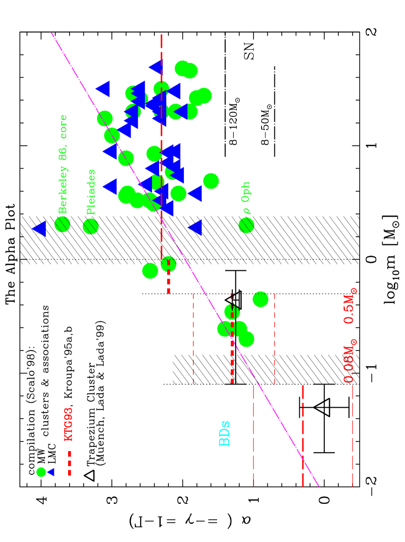
The models discussed in Section 5 show that unresolved binary systems mostly affect the region $m\mbox{$\,\mathrel{\mathchoice{{\mbox{\lower 2.15277pt\vbox{\halign{$\mathsurround=0pt \displaystyle\hfil#\hfil$\cr<\crcr\sim\crcr}}}}}{{\mbox{\lower 2.15277pt\vbox{\halign{$\mathsurround=0pt \textstyle\hfil#\hfil$\cr<\crcr\sim\crcr}}}}}{{\mbox{\lower 2.15277pt\vbox{\halign{$\mathsurround=0pt \scriptstyle\hfil#\hfil$\cr<\crcr\sim\crcr}}}}}{{\mbox{\lower 2.15277pt\vbox{\halign{$\mathsurround=0pt \scriptscriptstyle\hfil#\hfil$\cr<\crcr\sim\crcr}}}}}}\,$}1\,M_{\odot}$, the data for which are listed in Table 1. Perusal of the references shows that only Meusinger et al. (1996) attempted a correction for unresolved binary systems. However, they adopted an artificial model of Reid (1991; see discussion in Kroupa 1995a), in which the binary proportion is only 40 per cent, half of which have similar companion masses. This is an unrealistic model (Kähler 1999), and leads to essentially no difference between the system and single-star LFs (fig. 7 in Meusinger et al. 1996, compare with fig. 11 in Kroupa 1995d). Their binary correction can thus be safely neglected.

log${}_{10}m_{\rm av}$	$\alpha$	cluster	ref.
$-0.70$	1.10	$\rho$ Oph	(Williams et al. 1995b)
$-0.61$	1.40	$\rho$ Oph	(Comeron, Rieke & Rieke 1996)
$-0.61$	1.20	NGC 2024	(Comeron, Rieke & Rieke 1996)
$-0.46$	1.30	Praesepe	(Williams, Rieke & Stauffer 1995a)
$-0.35$	1.10	Pleiades	(Meusinger et al. 1996)
$-0.10$	2.46	ONC	(Hillenbrand 1997)
$-0.04$	2.20	Praesepe	(Williams, Rieke & Stauffer 1995a)

Table 1:: The data from Scalo’s (1998) compilation with $m_{\rm av}<1\,M_{\odot}$.

2.1.1 $m>3\,M_{\odot}$

For $m\mbox{$\,\mathrel{\mathchoice{{\mbox{\lower 2.15277pt\vbox{\halign{$\mathsurround=0pt \displaystyle\hfil#\hfil$\cr>\crcr\sim\crcr}}}}}{{\mbox{\lower 2.15277pt\vbox{\halign{$\mathsurround=0pt \textstyle\hfil#\hfil$\cr>\crcr\sim\crcr}}}}}{{\mbox{\lower 2.15277pt\vbox{\halign{$\mathsurround=0pt \scriptstyle\hfil#\hfil$\cr>\crcr\sim\crcr}}}}}{{\mbox{\lower 2.15277pt\vbox{\halign{$\mathsurround=0pt \scriptscriptstyle\hfil#\hfil$\cr>\crcr\sim\crcr}}}}}}\,$}3\,M_{\odot}$ the data suggest that the Salpeter power-law value, $\alpha=2.3$, is a reasonable fit over the whole range, as is also stressed by Massey (1998). Massey & Hunter (1998), for example, deduce that $\alpha\approx 2.3$ for $2.8<m<120\,M_{\odot}$ in the massive cluster R136 in the LMC. This value is thus adopted throughout the rest of this paper, although notable examples of exotic clusters exist. The two massive, apparently young (2–4 Myr) Arches and Quintuplet clusters lying very close to the Galactic centre (projected distance 30 pc) have $\alpha\approx 1.65$ (Figer et al. 1999), and the Galactic star-burst template cluster NGC 3603 is found to have $\alpha\approx 1.7$ (Eisenhauer et al. 1998). Further work is desired to establish the exact nature of the central clusters, and clarify the age discrepancy between the low-mass and massive stars noted for NGC 3603, a problem possibly associated with pre-main sequence models.

It is important to keep in mind that $\alpha$ may be systematically steeper than $\alpha=2.3$ (or 1.7) due to unresolved binary systems, which are not usually corrected for in IMF estimates. The multiplicity proportion of massive stars is very high (Mason et al. 1998). For example, Preibisch et al. (1999) find that the OB stars in the well studied ONC have, on average, 1.5 companions. For each primary, there is thus usually more than one secondary that adds at lower masses, steepening the observed IMF when corrected for. The effect depends on $\alpha$, and Sagar & Richtler (1991) calculate that $\Delta\alpha=+0.34$ for $\alpha=2.5$ and a binary proportion $f=0.5$ (eq. 5 below). If $f=1$ (each massive primary has 1.0 companions) they obtain $\Delta\alpha=+0.40$. $\Delta\alpha$ is likely to be larger still, because each massive primary probably has more than one companion, typically. Since the empirical data in Fig. 1 implies an average $\alpha\approx 2.3$ for $m\mbox{$\,\mathrel{\mathchoice{{\mbox{\lower 2.15277pt\vbox{\halign{$\mathsurround=0pt \displaystyle\hfil#\hfil$\cr>\crcr\sim\crcr}}}}}{{\mbox{\lower 2.15277pt\vbox{\halign{$\mathsurround=0pt \textstyle\hfil#\hfil$\cr>\crcr\sim\crcr}}}}}{{\mbox{\lower 2.15277pt\vbox{\halign{$\mathsurround=0pt \scriptstyle\hfil#\hfil$\cr>\crcr\sim\crcr}}}}}{{\mbox{\lower 2.15277pt\vbox{\halign{$\mathsurround=0pt \scriptscriptstyle\hfil#\hfil$\cr>\crcr\sim\crcr}}}}}}\,$}3\,M_{\odot}$, the true single-star IMF may in fact have $\alpha\approx 2.7(=2.3+0.4)$, or even larger. A similar conclusion is reached by Scalo (1998, at the end of his section 4). Such corrections will not be removed if spectroscopic mass determinations are used instead of the inferior mass-estimates using photometry (Massey et al. 1995a), since unresolved systems will have similar effects on a spectroscopic sample.

In this paper the approximate average $\alpha=2.3$ is adopted, with the aim of studying the effect of unresolved binary systems on the $\alpha$ inferred from the system MF, which an observer would deduce from the mixture of single stars and binary systems in a population resulting from star-cluster evolution with initially $f=1$. Because the assumptions (Section 4.3) imply that massive stars have very-low mass companions in this model, and because only binary systems are searched for in the data reduction software, the resulting model bias will be an underestimate. Further work is necessary to address this particular issue, which is also discussed further at the end of Section 3 and in Section 4.4.

The remarkable feature for $m\mbox{$\,\mathrel{\mathchoice{{\mbox{\lower 2.15277pt\vbox{\halign{$\mathsurround=0pt \displaystyle\hfil#\hfil$\cr>\crcr\sim\crcr}}}}}{{\mbox{\lower 2.15277pt\vbox{\halign{$\mathsurround=0pt \textstyle\hfil#\hfil$\cr>\crcr\sim\crcr}}}}}{{\mbox{\lower 2.15277pt\vbox{\halign{$\mathsurround=0pt \scriptstyle\hfil#\hfil$\cr>\crcr\sim\crcr}}}}}{{\mbox{\lower 2.15277pt\vbox{\halign{$\mathsurround=0pt \scriptscriptstyle\hfil#\hfil$\cr>\crcr\sim\crcr}}}}}}\,$}3\,M_{\odot}$ in the alpha plot is the constant scatter, and that the various power-law indices are distributed more or less randomly throughout the region $\alpha=2.3\pm 0.7$ without a significant concentration towards some value.

2.1.2 $0.8<m<3\,M_{\odot}$

The region for $0.8\mbox{$\,\mathrel{\mathchoice{{\mbox{\lower 2.15277pt\vbox{\halign{$\mathsurround=0pt \displaystyle\hfil#\hfil$\cr<\crcr\sim\crcr}}}}}{{\mbox{\lower 2.15277pt\vbox{\halign{$\mathsurround=0pt \textstyle\hfil#\hfil$\cr<\crcr\sim\crcr}}}}}{{\mbox{\lower 2.15277pt\vbox{\halign{$\mathsurround=0pt \scriptstyle\hfil#\hfil$\cr<\crcr\sim\crcr}}}}}{{\mbox{\lower 2.15277pt\vbox{\halign{$\mathsurround=0pt \scriptscriptstyle\hfil#\hfil$\cr<\crcr\sim\crcr}}}}}}\,$}m\mbox{$\,\mathrel{\mathchoice{{\mbox{\lower 2.15277pt\vbox{\halign{$\mathsurround=0pt \displaystyle\hfil#\hfil$\cr<\crcr\sim\crcr}}}}}{{\mbox{\lower 2.15277pt\vbox{\halign{$\mathsurround=0pt \textstyle\hfil#\hfil$\cr<\crcr\sim\crcr}}}}}{{\mbox{\lower 2.15277pt\vbox{\halign{$\mathsurround=0pt \scriptstyle\hfil#\hfil$\cr<\crcr\sim\crcr}}}}}{{\mbox{\lower 2.15277pt\vbox{\halign{$\mathsurround=0pt \scriptscriptstyle\hfil#\hfil$\cr<\crcr\sim\crcr}}}}}}\,$}3\,M_{\odot}$ shows an unusually large scatter. It is shaded because this particular mass range is problematical for a number of reasons.

Analysis of Galactic-field star-counts run into the difficulty that the age of the Galactic disk is comparable to the life-time of these stars so that stellar evolution corrections become very significant, but for this the sfh must be known (Scalo 1986; Haywood, Robin & Crézé 1997). That interesting constraints can be placed on the MW IMF using independently derived sfhs is shown by Maciel & Rocha-Pinto (1998), where the problems associated with the estimation of the field-IMF for massive stars are documented.

The large spread of the cluster values in the region $0.8\mbox{$\,\mathrel{\mathchoice{{\mbox{\lower 2.15277pt\vbox{\halign{$\mathsurround=0pt \displaystyle\hfil#\hfil$\cr<\crcr\sim\crcr}}}}}{{\mbox{\lower 2.15277pt\vbox{\halign{$\mathsurround=0pt \textstyle\hfil#\hfil$\cr<\crcr\sim\crcr}}}}}{{\mbox{\lower 2.15277pt\vbox{\halign{$\mathsurround=0pt \scriptstyle\hfil#\hfil$\cr<\crcr\sim\crcr}}}}}{{\mbox{\lower 2.15277pt\vbox{\halign{$\mathsurround=0pt \scriptscriptstyle\hfil#\hfil$\cr<\crcr\sim\crcr}}}}}}\,$}m\mbox{$\,\mathrel{\mathchoice{{\mbox{\lower 2.15277pt\vbox{\halign{$\mathsurround=0pt \displaystyle\hfil#\hfil$\cr<\crcr\sim\crcr}}}}}{{\mbox{\lower 2.15277pt\vbox{\halign{$\mathsurround=0pt \textstyle\hfil#\hfil$\cr<\crcr\sim\crcr}}}}}{{\mbox{\lower 2.15277pt\vbox{\halign{$\mathsurround=0pt \scriptstyle\hfil#\hfil$\cr<\crcr\sim\crcr}}}}}{{\mbox{\lower 2.15277pt\vbox{\halign{$\mathsurround=0pt \scriptscriptstyle\hfil#\hfil$\cr<\crcr\sim\crcr}}}}}}\,$}3\,M_{\odot}$ may be due to the fact that the observed clusters have ages such that the stars in this mass range count to the most massive remaining in the clusters. They are thus subject to advanced stellar evolution and/or dynamical ejection from the cluster, because the most massive stars usually interact in the vicinity of the cluster core. Which of these is applicable is a sensitive function of the age of the cluster and the number of stars in it (more on this in Section 5.2). Finally, stellar evolution is by no means a solved subject for stars in this mass range (Dominguez et al. 1999) with remaining significant uncertainties. This compromises the conversion of stellar luminosity to mass. Ignoring the large scatter in this mass range, it can be seen that a single power-law index becomes applicable for $m>0.5\,M_{\odot}$.

2.1.3 $0.1<m<1\,M_{\odot}$

The Galactic-field single-star IMF fits the data shown in Fig. 1 exceedingly well for $0.1<m<1\,M_{\odot}$ (that this agreement may be fortuitous though is shown in Section 6.2). In particular, it is remarkable that the data suggest a change in $\alpha$ near $0.5\,M_{\odot}$, as was initially derived from solar-neighbourhood star-counts by Kroupa, Tout & Gilmore (1991, hereinafter KTG91), and later confirmed by Kroupa, Tout & Gilmore (1993, hereinafter KTG93) and Kroupa (1995a) using a different mass–luminosity relation, a much more detailed star-count analysis including main-sequence and pre-main sequence stellar evolution, and with different statistical tests. Similar work by Gould, Bahcall & Flynn (1997) using HST star-counts and Reid & Gizis (1997), who study a proposed extension of the nearby stellar sample to somewhat larger distances, also confirm these findings, as do Chabrier & Baraffe (2000), who estimate $\alpha\approx 1.2\pm 0.1$ using the nearby volume-limited LF.

Of special importance is the mass range $0.5-1\,M_{\odot}$: The local sample of known stars is sufficiently large in this mass range that the nearby volume-limited LF is very well defined (Kroupa 2001a). Also, unresolved binaries do not significantly affect the LF in this mass range, because the stellar sample does not contain stars with $m>1\,M_{\odot}$ that can hide lower-mass companions. The mass–luminosity relation is also well understood for these stars, so that the MF determination should be accurate and precise. It is not surprising that the power-law slope has changed little over the decades (Salpeter 1955: $\alpha=2.35$ for $0.4<m<10\,M_{\odot}$). From Fig. 1 an uncertainty of $\alpha=2.3\pm 0.3$ is adopted.

Unfortunately, the local sample of stars with $m\mbox{$\,\mathrel{\mathchoice{{\mbox{\lower 2.15277pt\vbox{\halign{$\mathsurround=0pt \displaystyle\hfil#\hfil$\cr<\crcr\sim\crcr}}}}}{{\mbox{\lower 2.15277pt\vbox{\halign{$\mathsurround=0pt \textstyle\hfil#\hfil$\cr<\crcr\sim\crcr}}}}}{{\mbox{\lower 2.15277pt\vbox{\halign{$\mathsurround=0pt \scriptstyle\hfil#\hfil$\cr<\crcr\sim\crcr}}}}}{{\mbox{\lower 2.15277pt\vbox{\halign{$\mathsurround=0pt \scriptscriptstyle\hfil#\hfil$\cr<\crcr\sim\crcr}}}}}}\,$}0.5\,M_{\odot}$ is incomplete for distances larger than $d\approx 5$ pc, in contradiction to the belief by Reid & Gizis (1997), who use spectroscopic parallax measurements to extend their proposed volume-limited sample using previously-known stars. Malmquist bias pollutes their sample by multiple systems that are much further away. The seriousness of the incompleteness of the nearby stellar census is shown by Henry et al. (1997), and is also pointed out by Chabrier & Baraffe (2000). This situation can only be improved with large-scale and deep surveys that find candidate nearby M dwarfs with subsequent trigonometric parallax measurements to affirm the distance, such that a volume limited sample can be constructed. This will be possible through the upcoming astrometric space missions DIVA (Röser 1999) and GAIA (Gilmore et al. 1998). Being aware of this situation, the KTG studies combined the local ($d\leq 5.2$ pc) volume limited sample with flux limited deep photometric surveys, performing detailed Monte Carlo modelling of both Galactic-field samples. This pedantic separation of the two star-count samples is necessary as completely different biases and errors operate. The result is the conservative uncertainty range of $\alpha=1.3\pm 0.5$ for $0.08-0.5\,M_{\odot}$ (KTG93). That the Galactic-bulge MF shows an indistinguishable behaviour to the Galactic-field MF in this mass range was already pointed out in Section 1.

2.1.4 $m<0.08\,M_{\odot}$

For sub-stellar masses the constraints have improved dramatically in the past few years as a result of the significant observational effort and instrumental advances. In the ONC, Muench, Lada & Lada (2000) and Hillenbrand & Carpenter (2000) find $-1\mbox{$\,\mathrel{\mathchoice{{\mbox{\lower 2.15277pt\vbox{\halign{$\mathsurround=0pt \displaystyle\hfil#\hfil$\cr<\crcr\sim\crcr}}}}}{{\mbox{\lower 2.15277pt\vbox{\halign{$\mathsurround=0pt \textstyle\hfil#\hfil$\cr<\crcr\sim\crcr}}}}}{{\mbox{\lower 2.15277pt\vbox{\halign{$\mathsurround=0pt \scriptstyle\hfil#\hfil$\cr<\crcr\sim\crcr}}}}}{{\mbox{\lower 2.15277pt\vbox{\halign{$\mathsurround=0pt \scriptscriptstyle\hfil#\hfil$\cr<\crcr\sim\crcr}}}}}}\,$}\alpha\mbox{$\,\mathrel{\mathchoice{{\mbox{\lower 2.15277pt\vbox{\halign{$\mathsurround=0pt \displaystyle\hfil#\hfil$\cr<\crcr\sim\crcr}}}}}{{\mbox{\lower 2.15277pt\vbox{\halign{$\mathsurround=0pt \textstyle\hfil#\hfil$\cr<\crcr\sim\crcr}}}}}{{\mbox{\lower 2.15277pt\vbox{\halign{$\mathsurround=0pt \scriptstyle\hfil#\hfil$\cr<\crcr\sim\crcr}}}}}{{\mbox{\lower 2.15277pt\vbox{\halign{$\mathsurround=0pt \scriptscriptstyle\hfil#\hfil$\cr<\crcr\sim\crcr}}}}}}\,$}1$, although the pre-main sequence tracks are unreliable at these ages. Similarly, in $\rho$ Oph Luhman & Rieke (1999) estimate $\alpha\approx 0.5$, which is also found for IC348 by Najita, Tiede & Carr (2000). In the Pleiades Cluster, Martin et al. (2000) estimate $\alpha\approx 0.53$, and for the solar neighbourhood, Reid et al. (1999) quote $1\mbox{$\,\mathrel{\mathchoice{{\mbox{\lower 2.15277pt\vbox{\halign{$\mathsurround=0pt \displaystyle\hfil#\hfil$\cr<\crcr\sim\crcr}}}}}{{\mbox{\lower 2.15277pt\vbox{\halign{$\mathsurround=0pt \textstyle\hfil#\hfil$\cr<\crcr\sim\crcr}}}}}{{\mbox{\lower 2.15277pt\vbox{\halign{$\mathsurround=0pt \scriptstyle\hfil#\hfil$\cr<\crcr\sim\crcr}}}}}{{\mbox{\lower 2.15277pt\vbox{\halign{$\mathsurround=0pt \scriptscriptstyle\hfil#\hfil$\cr<\crcr\sim\crcr}}}}}}\,$}\alpha\mbox{$\,\mathrel{\mathchoice{{\mbox{\lower 2.15277pt\vbox{\halign{$\mathsurround=0pt \displaystyle\hfil#\hfil$\cr<\crcr\sim\crcr}}}}}{{\mbox{\lower 2.15277pt\vbox{\halign{$\mathsurround=0pt \textstyle\hfil#\hfil$\cr<\crcr\sim\crcr}}}}}{{\mbox{\lower 2.15277pt\vbox{\halign{$\mathsurround=0pt \scriptstyle\hfil#\hfil$\cr<\crcr\sim\crcr}}}}}{{\mbox{\lower 2.15277pt\vbox{\halign{$\mathsurround=0pt \scriptscriptstyle\hfil#\hfil$\cr<\crcr\sim\crcr}}}}}}\,$}2$, whereas Herbst et al. (1999) estimate $\alpha<0.8$ with 90 per cent confidence on the basis of no detections but accounting correctly for Galactic structure. For the time-being, $\alpha=0.3\pm 0.7$ is a reasonable description of the IMF for BDs, and it will be shown in Section 5.2 that the observed MF depends sensitively on the dynamical age of the population.

The region $0.08-0.15\,M_{\odot}$ is shaded in Fig. 1 to emphasise the uncertainties plaguing Galactic-field star-count interpretations as a result of the long pre-main sequence contraction times for these stars. As with the $0.8-3\,M_{\odot}$ region, the sfh must be known. The sfh has most recently been constrained by Rocha-Pinto et al (2000).

2.2 The universal IMF

The available constraints can be conveniently summarised by the multiple-part power-law IMF (see Kroupa 2001b for details),

$$\xi(m)\propto m^{-\alpha_{i}}=m^{\gamma_{i}},$$ (1)

where

$$\begin{array}[]{l@{\quad\quad,\quad}l}\alpha_{0}=+0.3\pm 0.7&0.01\leq m/M_{\odot}<0.08,\\ \alpha_{1}=+1.3\pm 0.5&0.08\leq m/M_{\odot}<0.50,\\ \alpha_{2}=+2.3\pm 0.3&0.50\leq m/M_{\odot}<1.00,\\ \alpha_{3}=+2.3\pm 0.7&1.00\leq m/M_{\odot},\\ \end{array}$$ (2)

and $\xi(m)\,dm$ is the number of single stars in the mass interval $m$ to $m+dm$. The uncertainties correspond approximately to 99 per cent confidence intervals for $m\mbox{$\,\mathrel{\mathchoice{{\mbox{\lower 2.15277pt\vbox{\halign{$\mathsurround=0pt \displaystyle\hfil#\hfil$\cr>\crcr\sim\crcr}}}}}{{\mbox{\lower 2.15277pt\vbox{\halign{$\mathsurround=0pt \textstyle\hfil#\hfil$\cr>\crcr\sim\crcr}}}}}{{\mbox{\lower 2.15277pt\vbox{\halign{$\mathsurround=0pt \scriptstyle\hfil#\hfil$\cr>\crcr\sim\crcr}}}}}{{\mbox{\lower 2.15277pt\vbox{\halign{$\mathsurround=0pt \scriptscriptstyle\hfil#\hfil$\cr>\crcr\sim\crcr}}}}}}\,$}0.5\,M_{\odot}$ (Fig. 1), and to a 95 per cent confidence interval for $0.1-0.5\,M_{\odot}$ (KTG93). Below $0.08\,M_{\odot}$ the confidence range is not well determined.

Note that this form differs from Scalo’s (1998) recommendation, mostly because the correct structure in the luminosity function below $1\,M_{\odot}$ is accounted for here. There is evidence for only two changes in the power-law index, namely near $0.5\,M_{\odot}$ and near $0.08\,M_{\odot}$. The frequently used Miller & Scalo (1979) IMF fails in the region $0.5-1\,M_{\odot}$, and especially for $m\mbox{$\,\mathrel{\mathchoice{{\mbox{\lower 2.15277pt\vbox{\halign{$\mathsurround=0pt \displaystyle\hfil#\hfil$\cr>\crcr\sim\crcr}}}}}{{\mbox{\lower 2.15277pt\vbox{\halign{$\mathsurround=0pt \textstyle\hfil#\hfil$\cr>\crcr\sim\crcr}}}}}{{\mbox{\lower 2.15277pt\vbox{\halign{$\mathsurround=0pt \scriptstyle\hfil#\hfil$\cr>\crcr\sim\crcr}}}}}{{\mbox{\lower 2.15277pt\vbox{\halign{$\mathsurround=0pt \scriptscriptstyle\hfil#\hfil$\cr>\crcr\sim\crcr}}}}}}\,$}5\,M_{\odot}$ (Fig. 1, see also Fig. 14 below). A useful representation of the IMF is achieved via the logarithmic form,

$$\xi_{\rm L}(m)={\xi(m)\,{\rm ln}10\,m},$$ (3)

where $\xi_{\rm L}\,d{\rm log}_{10}m\propto m^{\Gamma_{i}}\,d{\rm log}_{10}m=m^{-x_{i}}\,d{\rm log}_{10}m$ is the number of stars in the logarithmic mass interval log${}_{10}m$ to log${}_{10}m+d{\rm log}_{10}m$.

The adopted IMF (eq. 2) has a mean stellar mass $<m>=0.36\,M_{\odot}$ for stars with $0.01\leq m\leq 50\,M_{\odot}$, and leads to the following stellar population: 37 % BDs ($0.01-0.08\,M_{\odot}$) contributing 4.3 % to the stellar mass, 48 % M dwarfs ($0.08-0.5\,M_{\odot}$) contributing 28 % mass, 8.9 % “K” dwarfs ($0.5-1.0\,M_{\odot}$) contributing 17 % mass, 5.7 % “intermediate mass (IM) stars” ($1.0-8.0\,M_{\odot}$) contributing 34 % mass, and 0.37 % “O” stars ($>8\,M_{\odot}$) contributing 17 % mass.

A remarkable property of eq. 2 is that 50 per cent of the mass is in stars with $0.01\leq m\leq 1\,M_{\odot}$ and 50 per cent in stars with $1-50\,M_{\odot}$. Also, if $\alpha_{4}=0.70$ ($m>8\,M_{\odot}$) then 50 per cent of the mass is in stars with $8\leq m\leq 50\,M_{\odot}$, whereas $\alpha_{4}=1.4$ implies 50 per cent mass in $8-120\,M_{\odot}$ stars. These numbers are useful for the evolution of star clusters, because supernovae (SN) lead to rapid mass loss which can unbind a cluster if too much mass resides in the SN precursors. This is the case in clusters that have $\alpha_{3}=1.80$: stars with $8<m\leq 120\,M_{\odot}$ contain 53 per cent of the mass in the stellar population! It is interesting that $\alpha\approx 1.8$ for $m\mbox{$\,\mathrel{\mathchoice{{\mbox{\lower 2.15277pt\vbox{\halign{$\mathsurround=0pt \displaystyle\hfil#\hfil$\cr>\crcr\sim\crcr}}}}}{{\mbox{\lower 2.15277pt\vbox{\halign{$\mathsurround=0pt \textstyle\hfil#\hfil$\cr>\crcr\sim\crcr}}}}}{{\mbox{\lower 2.15277pt\vbox{\halign{$\mathsurround=0pt \scriptstyle\hfil#\hfil$\cr>\crcr\sim\crcr}}}}}{{\mbox{\lower 2.15277pt\vbox{\halign{$\mathsurround=0pt \scriptscriptstyle\hfil#\hfil$\cr>\crcr\sim\crcr}}}}}}\,$}1\,M_{\odot}$ forms the lower bound on the empirical data in Fig. 1. But even ’normal’ ($\alpha=2.3$) star clusters suffer seriously through the evolution of their $m>1\,M_{\odot}$ stars (de La Fuente Marcos 1997).

3 PROCEDURE AND STATISTICAL VARIATION

One contribution to the scatter seen in the alpha-plot (Fig. 1) is Poisson noise. This can be studied by sampling $N$ stars from the adopted IMF (eq. 2), and studying the variation of $\alpha$ with $N$.

In order to construct synthetic alpha-plots, the following procedure is adopted. $N$ masses are obtained by randomly sampling eq. 2 with lower mass limit $m_{\rm l}=0.01\,M_{\odot}$ and upper mass limit $m_{\rm u}=50\,M_{\odot}$. This upper mass limit is chosen for consistency with the stellar-dynamical models (Section 4). The MF is constructed by binning the masses, $m$, into 30 log${}_{10}m$ bins which subdivide the range $-2.1\leq{\rm log}_{10}m\leq+2.1$. Power-laws are fitted using weighted linear regression (e.g. Press et al. 1994) to sub-ranges that are defined as follows:

$$\begin{array}[]{ll@{\quad\quad,\quad}l}b1&6&{\rm log}_{10}(0.01)<{\rm l}m\leq{\rm log}_{10}(0.08),\\ b2&6&{\rm log}_{10}(0.08)<{\rm l}m\leq{\rm log}_{10}(0.50),\\ b3&4&{\rm log}_{10}(0.40)<{\rm l}m\leq{\rm log}_{10}(1.20),\\ b4&4&{\rm log}_{10}(1.00)<{\rm l}m\leq{\rm log}_{10}(3.50),\\ b5&4&{\rm log}_{10}(3.00)<{\rm l}m\leq{\rm log}_{10}(9.00),\\ b6&8&{\rm log}_{10}(5.00)<{\rm l}m,\\ \end{array}$$ (4)

where ${\rm l}m={\rm log}_{10}m/M_{\odot}$, and the numbers, $nb$, behind the mass-range number (e.g. $b1$) are the number of mass bins in the histogram in that particular mass range (e.g. $nb_{1}=6$). This sub-division ensures that the different mass regions in which $\alpha_{i}$ is known to be constant (eq. 2) are not mixed up, but also allows studying the fitted $\alpha$ at values of ${\rm l}m$ where, for example, stellar evolution and/or dynamical effects are expected to be important. The result is $\alpha({\rm l}m_{\rm av})$, where ${\rm l}m_{\rm av}$ is the average of ${\rm l}m$ over the $nb_{j}$ ($j=1,6$) bins. In cases where the number of stars is too small, or the highest mass star is less massive than $10^{2.1}\,M_{\odot}$, some of the highest-mass bins remain empty, causing ${\rm l}m_{\rm av}$ in mass-range $b6$ to vary between renditions.

The IMF is plotted together with two renditions using $N=10^{3}$ stars in Fig. 3, to illustrate the procedure. The resulting alpha-plot is shown in Fig. 3 for many more renditions and different $N$. The input IMF is obtained essentially exactly for $N=10^{6}$ and $10^{5}$, verifying the procedure. The figure shows that deviations begin to occur for $N=10^{4}$ in the two highest mass-ranges ($b5$ and $b6$), because these contain only a few per cent of $N$, i.e. a few hundred stars, spread over about 10 mass bins. For smaller $N$ the scatter of $\alpha({\rm l}m_{\rm av})$ becomes larger, with the average reproducing the IMF except when the MF is under-sampled at large masses.

Fig. 2.—: The adopted logarithmic IMF (eqs. 2 and 3), $\xi_{\rm L}/10^{3}$, for $10^{6}$ stars (solid histogram). Two random renditions of this IMF with $10^{3}$ stars are shown as the heavy and thin dotted histograms. The mass-ranges over which power-law functions are fitted are indicated by the arrowed six regions (eq. 4), while thin vertical dotted lines indicate the masses at which $\alpha_{i}$ changes.

Fig. 3.—: Purely statistical variation of $\alpha$ in the six mass ranges (eq. 4) for different $N$ as indicated in the key. Large outer squares indicate those $\alpha$ fits obtained with $nb=2$ and 3 mass bins. The open circles, open triangles, vertical and horizontal lines are as in Fig. 1.

Fig. 3 illustrates this sampling bias. The under-sampling of the histogram in the highest mass bins, when $N$ is too small, leads to an apparent flattening of the MF in the most massive bins accessible to the stellar population, as is evident in Fig. 3. It is also evident in fig. 2 of Elmegreen (1999), and in typical star-count data, such as used by Massey et al. (1995b, their fig. 5) to infer the power-law index. Such samples contain typically a few dozen stars only (their table 5). This is interesting, possibly implying that the correct single-star IMF may be steepening, i.e. have an increasing $\alpha$, with l$m$ at the largest masses, since the uncorrected data suggest a constant $\alpha$ for $m\mbox{$\,\mathrel{\mathchoice{{\mbox{\lower 2.15277pt\vbox{\halign{$\mathsurround=0pt \displaystyle\hfil#\hfil$\cr>\crcr\sim\crcr}}}}}{{\mbox{\lower 2.15277pt\vbox{\halign{$\mathsurround=0pt \textstyle\hfil#\hfil$\cr>\crcr\sim\crcr}}}}}{{\mbox{\lower 2.15277pt\vbox{\halign{$\mathsurround=0pt \scriptstyle\hfil#\hfil$\cr>\crcr\sim\crcr}}}}}{{\mbox{\lower 2.15277pt\vbox{\halign{$\mathsurround=0pt \scriptscriptstyle\hfil#\hfil$\cr>\crcr\sim\crcr}}}}}}\,$}1\,M_{\odot}$. This issue, together with the bias through the high multiplicity fraction, will require more explicit modelling of the biases affecting the observed IMF for massive stars.

In conclusion, Fig. 3 demonstrates that the observed scatter is arrived at approximately for populations that contain $10^{2}\mbox{$\,\mathrel{\mathchoice{{\mbox{\lower 2.15277pt\vbox{\halign{$\mathsurround=0pt \displaystyle\hfil#\hfil$\cr<\crcr\sim\crcr}}}}}{{\mbox{\lower 2.15277pt\vbox{\halign{$\mathsurround=0pt \textstyle\hfil#\hfil$\cr<\crcr\sim\crcr}}}}}{{\mbox{\lower 2.15277pt\vbox{\halign{$\mathsurround=0pt \scriptstyle\hfil#\hfil$\cr<\crcr\sim\crcr}}}}}{{\mbox{\lower 2.15277pt\vbox{\halign{$\mathsurround=0pt \scriptscriptstyle\hfil#\hfil$\cr<\crcr\sim\crcr}}}}}}\,$}N\mbox{$\,\mathrel{\mathchoice{{\mbox{\lower 2.15277pt\vbox{\halign{$\mathsurround=0pt \displaystyle\hfil#\hfil$\cr<\crcr\sim\crcr}}}}}{{\mbox{\lower 2.15277pt\vbox{\halign{$\mathsurround=0pt \textstyle\hfil#\hfil$\cr<\crcr\sim\crcr}}}}}{{\mbox{\lower 2.15277pt\vbox{\halign{$\mathsurround=0pt \scriptstyle\hfil#\hfil$\cr<\crcr\sim\crcr}}}}}{{\mbox{\lower 2.15277pt\vbox{\halign{$\mathsurround=0pt \scriptscriptstyle\hfil#\hfil$\cr<\crcr\sim\crcr}}}}}}\,$}10^{3}$ stars, which is quite typical for the type of samples available.

4 STAR CLUSTER MODELS

In Section 3 apparent variations of the IMF are discussed that result purely from statistical fluctuations. Additional sources of uncertainty are listed in the Introduction. Section 5 concentrates on quantifying the apparent variations that arise from stellar-dynamical effects and unresolved binary systems. To achieve this, a range of star-cluster models are constructed. This approach is relevant to populations in young clusters, OB associations and even the Galactic field, because most stars form in embedded clusters (Lada & Lada 1991; Kroupa 1995b).

4.1 Codes

The dynamical evolution of the clusters studied here is calculated using Nbody6 (Aarseth 1999; Aarseth 2000), which includes state-of-the art stellar evolution (Hurley, Pols & Tout 2000), a standard Galactic tidal field (Terlevich 1987), and additional routines for initiating the binary-rich population (Kroupa 1995c). The $N$-body data are analysed with a large data-reduction programme that calculates, among many quantities, the binary proportion and MFs.

4.2 The clusters

The cluster models are set-up to have the same central density, $\rho_{\rm C}=10^{4.8}$ stars/pc³, as observed in the Trapezium Cluster (McCaughrean & Stauffer 1994), giving a half-mass diameter crossing time $t_{\rm cross}=0.24$ Myr. The centre of masses of the binary systems follow a Plummer density distribution (Aarseth, Hénon & Wielen 1974) with half-mass radius $R_{0.5}$. The average stellar mass is independent of the radial distance, $R$, from the cluster centre, and the clusters are in virial equilibrium. Their parameters are listed in Table 2. Cluster evolution is followed for 150 Myr.

model	$N$	$N_{\rm bin}$	$R_{0.5}$	$<\!\!m\!\!>$	$\sigma_{\rm 3D}$	$t_{\rm rel}$	$N_{\rm run}$
			[pc]	[$M_{\odot}$]	[km/s]	[Myr]
B800	800	400	0.19	0.4	1.6	0.8–1.4	5
B3000	3000	1500	0.30	0.4	2.5	2.4–4.4	5
B1E4	$10^{4}$	5000	0.45	0.4	3.7	6.8–12.5	2
B1E4d	$10^{4}$	5000	0.45	0.3	3.2	7.9–14.5	2

Table 2:: Cluster models: $N$ and $N_{\rm bin}$ are the initial number of stars and binaries in each model (not taking into account mergers), $R_{0.5}$ is the half-mass radius, and $<\!\!m\!\!>$ is the average stellar mass. The three-dimensional velocity dispersion is $\sigma_{\rm 3D}$, the median relaxation-time is $t_{\rm rel}$. It’s range results from assuming $f=1$ and $f=0$, respectively, since $f$ evolves. The number of calculations per model is $N_{\rm run}$. Model B1E4d has $\alpha_{3}=2.7$ ($m>1\,M_{\odot}$, eq. 2), whereas the other (default) models have $\alpha_{3}=\alpha_{2}=2.3$. It took about 4 months to assemble these data on standard desk-top computers.

4.3 The stellar population

Stellar masses are distributed according to the IMF (eq. 2) with $m_{\rm l}=0.01\,M_{\odot}$ and $m_{\rm u}=50\,M_{\odot}$. This upper mass limit is half as large as the upper limit on the mass range used to evaluate the MF (eq. 4), to take into account stellar mergers. Merging can occur during pre-main sequence eigenevolution, as detailed below. The default models assume $\alpha_{3}=\alpha_{2}$, but one model is also constructed with the possibly more realistic value $\alpha_{3}=2.7$ (this model has $\alpha_{0}=0.5$ for historical reasons).

Binaries are created by pairing the stars randomly. The binary proportion is

$$f={N_{\rm bin}\over N_{\rm sing}+N_{\rm bin}},$$ (5)

where $N_{\rm sing}$ and $N_{\rm bin}$ are the number of single-star and binary systems, respectively. A birth binary proportion $f=1$ is assumed. The initial mean system mass is $2<\!\!m\!\!>$, with $<\!\!m\!\!>$ being the average stellar mass. This results in an approximately flat mass-ratio distribution (fig. 12 in Kroupa 1995c). Note however that encounters in clusters lead to the preferred disruption of binaries with low-mass companions. The initially “random” mass-ratio distribution evolves rapidly towards a distribution in which low-mass companions are less frequent, but still preferred (Kroupa 1995c). This is consistent with observations in that G-dwarf primaries (Duquennoy & Mayor 1991), Cepheids ($4-9\,M_{\odot}$, Evans 1995) and possibly OB stars (Mason et al. 1998; Preibisch et al. 1999) prefer low-mass companions.

Periods and eccentricities are distributed following Kroupa (1995c). The periods range from about 1 d to $10^{9}$ d, and pre-main sequence eigenevolution changes the periods, mass ratios and eccentricities such that they are consistent with observational constraints for late-type main sequence stars with short periods. Eigenevolution is the collective name for system-internal processes that evolve the orbital parameters, such as tidal circularisation, mass transfer, and interactions with circum-stellar and circum-binary discs. One feature of the pre-main sequence eigenevolution model is that secondary companions gain mass during accretion if the peri-astron distance is smaller than a critical value. This affects the IMF by slightly reducing the number of low-mass stars, and slightly increasing the number of massive stars. Also, in some rare cases the binary companions merge giving $N_{\rm sing}>0$, so that the true initial binary proportion is less than unity. Since only short-period binaries are affected by eigenevolution, the overall changes to the IMF are not significant.

The resulting single-star and system MFs are shown in Fig. 4. This figure demonstrates that the IMF that results from the eigenevolution model has a slightly smaller $\alpha$, especially for $m<0.5\,M_{\odot}$ (thick solid histogram). This effect is larger for the default case ($\alpha_{3}=2.3$), because the larger number of massive stars implies more systems in which the secondary gains mass as a result of eigenevolution. The effect on $\alpha$ is too small, however, to make a significant difference in the alpha-plot (e.g. Fig. 9 below). Fig. 4 also displays the large difference between the system MF and the single-star MF at low masses. The IMF has a maximum near $0.1\,M_{\odot}$, whereas the system MF has one near $0.4\,M_{\odot}$, and underestimates the number of ’stars’ by an order of magnitude near $m=0.01\,M_{\odot}$, and by a factor of three near $m=0.08\,M_{\odot}$.

Fig. 4.—: Mass functions for single-stars (solid histograms) and systems (dash-dotted histograms) at $t=0$ in models B1E4 (thick histograms) and B1E4d (thin histograms). Note the smaller number of massive stars in model B1E4d, which has a steeper IMF for $m>1\,M_{\odot}$ with $\alpha_{3}=2.7$ (Table 2). The solid dots are the IMF for $N=10^{6}$ stars (Fig. 3) scaled to $N=10^{4}$, and the vertical dotted lines and arrowed regions are as in Fig. 3.

4.4 Nota bene

The cluster models constructed here are extremes, in that they have a very high central density equal to that observed in the ONC. This assumption leads to a rapid depletion of the binary population, as shown below (Fig. 6; see also de La Fuente Marcos 1997). Disruption of binaries occurs on a crossing-time scale (Kroupa 2000a) in any cluster, so that it takes much longer in real time for the binary population to decrease in a Pleiades-type cluster, for which Kähler (1999) shows that $f\approx 0.7$ is possible. Likewise, the pre-main-sequence cluster IC348, which has a density of about 500 stars/pc³, has a binary proportion similar to that in the Galactic field (Duchene, Bouvier & Simon 1999). As shown by KTG91, such a binary proportion requires significant correction to the observed system LF to infer the IMF. The problem with unresolved binaries may be even worse for lower-density clusters still, such as studied by Testi, Palla & Natta (1999), because the binary population evolves on much longer time-scales, and is thus likely to be less evolved than in the clusters studied here. The problem will never be smaller in such clusters, unless they consist of a stellar population that had an unusually small initial binary proportion ($f<0.3$), i.e. smaller than even in the evolved extreme models here. Such a population has never been observed in any Galactic cluster or association to this date (e.g. Ghez et al. 1997; Duchene 1999).

Any real population is thus likely to have a larger binary proportion than in the models considered here after about three crossing times ($\approx 0.8$ Myr). In addition, the present results will be an underestimate of the bias, because only binary systems are considered. Real populations contain something like 20 per cent or more triple and quadruple systems, which, when not resolved, increase the systematic error made in the observational estimate of $\alpha$. What is inferred in this paper is thus the minimum correction to $\mathbf{\alpha}$.

This is particularly true for $m\mbox{$\,\mathrel{\mathchoice{{\mbox{\lower 2.15277pt\vbox{\halign{$\mathsurround=0pt \displaystyle\hfil#\hfil$\cr>\crcr\sim\crcr}}}}}{{\mbox{\lower 2.15277pt\vbox{\halign{$\mathsurround=0pt \textstyle\hfil#\hfil$\cr>\crcr\sim\crcr}}}}}{{\mbox{\lower 2.15277pt\vbox{\halign{$\mathsurround=0pt \scriptstyle\hfil#\hfil$\cr>\crcr\sim\crcr}}}}}{{\mbox{\lower 2.15277pt\vbox{\halign{$\mathsurround=0pt \scriptscriptstyle\hfil#\hfil$\cr>\crcr\sim\crcr}}}}}}\,$}1\,M_{\odot}$, because the observed mass-ratio distribution for massive stars (e.g. Preibisch et al. 1999) has secondaries that are typically more massive than $1\,M_{\odot}$, whereas in the models here, massive primaries typically have very low-mass companions owing to the random sampling hypothesis. This is very important when considering the system MFs below. It will be evident that the models lead to essentially no bias for massive stars, but this is more likely to be a shortcoming of the present assumptions, rather than proving that the IMF for massive systems is not subject to a significant bias, as discussed in Section 2.1.1. Clearly, this is a fundamentally important topic requiring much more work to construct a more realistic initial mass-ratio distribution for massive stars. In addition, a systematically different IMF between the LMC and the MW for massive stars may become evident, if the binary properties differ systematically between the two galaxies, because then the correction for systematic bias would be different for the two samples. At present no such difference is known, and so the empirical LMC and MW data plotted in Fig. 1 can, at present, be only taken to mean that the IMF for massive stars may be the same in the two populations.

5 RESULTS

The results obtained from the stellar-dynamical calculations are used to study temporal and spatial apparent variations of the single-star and system MFs.

5.1 Cluster evolution

As an impression of the evolution of the star clusters, Fig. 5 displays the scaled number of systems and single stars with $R\leq 3.2$ pc. $N_{\rm sys}(t)=N_{\rm sing}(t)+N_{\rm bin}(t)$ increases for $t\mbox{$\,\mathrel{\mathchoice{{\mbox{\lower 2.15277pt\vbox{\halign{$\mathsurround=0pt \displaystyle\hfil#\hfil$\cr<\crcr\sim\crcr}}}}}{{\mbox{\lower 2.15277pt\vbox{\halign{$\mathsurround=0pt \textstyle\hfil#\hfil$\cr<\crcr\sim\crcr}}}}}{{\mbox{\lower 2.15277pt\vbox{\halign{$\mathsurround=0pt \scriptstyle\hfil#\hfil$\cr<\crcr\sim\crcr}}}}}{{\mbox{\lower 2.15277pt\vbox{\halign{$\mathsurround=0pt \scriptscriptstyle\hfil#\hfil$\cr<\crcr\sim\crcr}}}}}}\,$}2.5$ Myr because the disruption of binary systems liberates secondaries. That is, the observer would find that the number of ’stars’ increases with time. After $t\approx 2.5$ Myr, $N_{\rm sys}$ decreases with a rate depending on $N$, because the clusters expand owing to binary-star heating, relaxation and mass-loss from evolving stars.

Fig. 5.—: Examples of the evolution of individual clusters. Top panel: The number of systems (thick curves) and all individual stars and BDs (thin curves) within the innermost 3.2 pc. The short-dashed lines are for $N=800$, the solid lines are for $N=3000$, and the dash-dotted lines are for $N=10^{4}$. Bottom panel: The binary proportion for $R\leq 3.2$ pc (thick curves), and all $R$ (thin curves) for the same cases as in top panel. In both panels, the horizontal dotted lines indicate the times (3 and 70 Myr) at which the mass functions are observed.

The binary proportion (Fig. 5) decreases within a few initial crossing times. The decay occurs on exactly the same time-scale for the different clusters, demonstrating that it is not the velocity dispersion in the cluster alone which dictates the disruptions, but the density as well. Owing to the ejection from the cluster of preferably single stars and because of mass segregation, $f$ is larger for systems with $R\leq 3.2$ pc and at times $t\mbox{$\,\mathrel{\mathchoice{{\mbox{\lower 2.15277pt\vbox{\halign{$\mathsurround=0pt \displaystyle\hfil#\hfil$\cr>\crcr\sim\crcr}}}}}{{\mbox{\lower 2.15277pt\vbox{\halign{$\mathsurround=0pt \textstyle\hfil#\hfil$\cr>\crcr\sim\crcr}}}}}{{\mbox{\lower 2.15277pt\vbox{\halign{$\mathsurround=0pt \scriptstyle\hfil#\hfil$\cr>\crcr\sim\crcr}}}}}{{\mbox{\lower 2.15277pt\vbox{\halign{$\mathsurround=0pt \scriptscriptstyle\hfil#\hfil$\cr>\crcr\sim\crcr}}}}}}\,$}2.5$ Myr, than for systems at larger distances from the clusters. The least massive clusters ($N=800$) have expanded appreciably by this time so that the remaining binary population in the cluster is hard, and no further significant disruption of binaries occurs ($f\approx 0.55$ and increasing for $t\mbox{$\,\mathrel{\mathchoice{{\mbox{\lower 2.15277pt\vbox{\halign{$\mathsurround=0pt \displaystyle\hfil#\hfil$\cr>\crcr\sim\crcr}}}}}{{\mbox{\lower 2.15277pt\vbox{\halign{$\mathsurround=0pt \textstyle\hfil#\hfil$\cr>\crcr\sim\crcr}}}}}{{\mbox{\lower 2.15277pt\vbox{\halign{$\mathsurround=0pt \scriptstyle\hfil#\hfil$\cr>\crcr\sim\crcr}}}}}{{\mbox{\lower 2.15277pt\vbox{\halign{$\mathsurround=0pt \scriptscriptstyle\hfil#\hfil$\cr>\crcr\sim\crcr}}}}}}\,$}2.5$ Myr). The more massive clusters, however, remain more concentrated for a longer time (top panel of Fig. 5), and consequently the binary-star hard/soft boundary remains at a higher binary binding energy for a longer time. At any time $t\mbox{$\,\mathrel{\mathchoice{{\mbox{\lower 2.15277pt\vbox{\halign{$\mathsurround=0pt \displaystyle\hfil#\hfil$\cr>\crcr\sim\crcr}}}}}{{\mbox{\lower 2.15277pt\vbox{\halign{$\mathsurround=0pt \textstyle\hfil#\hfil$\cr>\crcr\sim\crcr}}}}}{{\mbox{\lower 2.15277pt\vbox{\halign{$\mathsurround=0pt \scriptstyle\hfil#\hfil$\cr>\crcr\sim\crcr}}}}}{{\mbox{\lower 2.15277pt\vbox{\halign{$\mathsurround=0pt \scriptscriptstyle\hfil#\hfil$\cr>\crcr\sim\crcr}}}}}}\,$}3\,t_{\rm cross}\approx 0.7$ Myr, the binary proportion is higher in the clusters with smaller $N$, which his particularly evident in Fig. 6 below. This is a nice example of the caveat raised in Section 4.4. Further details on these processes are available in Kroupa (2000b), and in the seminal paper by Heggie (1975).

The evolution of the binary proportion for primaries with different masses is illustrated in Fig. 6. The binary proportion of BDs falls rapidly, and stabilises near $f_{\rm BD}=0.20$ in all models. M dwarfs retain a much higher binary proportion by $t=150$ Myr, $f_{\rm M}\approx 0.4-0.5$, depending on $N$, and more massive primaries retain a slightly higher binary proportion still. The overall binary proportion of O primaries ($m\geq 8\,M_{\odot}$) shows a complex behaviour. Initially, most O primaries have low-mass companions. These are, however, exchanged for more massive companions near the cluster core. When the primaries explode, these companions are left or are ejected as single stars. In addition, violent dynamical encounters in the cluster core eject single massive stars. Overall, $f_{\rm O}$ decays, but higher-order multiplicities that form in three-body encounters are not accounted for.

Fig. 6.—: The proportion of binaries with primary masses $>8\,M_{\odot}$, $f_{\rm O}$ (thick long-dash-dotted curve), $1-8\,M_{\odot}$, $f_{\rm IM}$ (thin short-dash-dotted curve), and $0.5-1\,M_{\odot}$, $f_{\rm K}$ (solid curve). M dwarf primaries ($0.08-0.5\,M_{\odot}$) have a binary proportion, $f_{\rm M}$ (thin dashed line), whereas brown dwarfs ($0.01-0.08\,M_{\odot}$), $f_{\rm BD}$, are shown as the thin dotted line. Each curve is an ensemble mean.

5.2 The alpha plot for cluster populations

Having briefly discussed the evolution of the clusters and of the binary population, the following question can now be posed: What MFs would an observer deduce if an ensemble of such clusters were observed at different times, under the extreme assumption that the mass of each star or system can be measured exactly?

Figs. 7 to 9 show the results for each $N$. The upper panels assume the observer sees all stars with $R\leq 3.2$ pc, whereas in the lower panel it is assumed that only the system masses can be measured exactly for systems with $R\leq 3.2$ pc. The MFs are constructed at times $t=0$, 3 Myr and 70 Myr. For the single-star MFs, the results at $t=0$ are the same as for pure statistical noise (Fig. 3).

Fig. 7.—: The $\alpha$-plot for five B800 models at $t=0$, 3 Myr (left panels) and 70 Myr (right panels). The single-star (top panels) and system (lower panels) MFs are constructed for stars with $R\leq 3.2$ pc. The open circles, open triangles, vertical and horizontal lines are as in Fig. 3.

Fig. 8.—: As Fig. 7, but for five B3000 models.

Fig. 9.—: As Fig. 7, but for models with $N=10^{4}$ stars. The crosses, four-pointed stars and squares are for the two B1E4 models, whereas the same symbols but rotated by 45 degrees are for the two B1E4d models.

At $t=0$, the single-star IMF is well reproduced. The system MF, on the other hand, underestimates $\alpha$ significantly for $m_{\rm sys}<1\,M_{\odot}$, with $\alpha_{0}\approx-0.8$ (instead of $+0.3$) for $m\mbox{$\,\mathrel{\mathchoice{{\mbox{\lower 2.15277pt\vbox{\halign{$\mathsurround=0pt \displaystyle\hfil#\hfil$\cr<\crcr\sim\crcr}}}}}{{\mbox{\lower 2.15277pt\vbox{\halign{$\mathsurround=0pt \textstyle\hfil#\hfil$\cr<\crcr\sim\crcr}}}}}{{\mbox{\lower 2.15277pt\vbox{\halign{$\mathsurround=0pt \scriptstyle\hfil#\hfil$\cr<\crcr\sim\crcr}}}}}{{\mbox{\lower 2.15277pt\vbox{\halign{$\mathsurround=0pt \scriptscriptstyle\hfil#\hfil$\cr<\crcr\sim\crcr}}}}}}\,$}0.08\,M_{\odot}$, $\alpha_{1}\approx+0.7$ (instead of $+1.3$) for $0.08\mbox{$\,\mathrel{\mathchoice{{\mbox{\lower 2.15277pt\vbox{\halign{$\mathsurround=0pt \displaystyle\hfil#\hfil$\cr<\crcr\sim\crcr}}}}}{{\mbox{\lower 2.15277pt\vbox{\halign{$\mathsurround=0pt \textstyle\hfil#\hfil$\cr<\crcr\sim\crcr}}}}}{{\mbox{\lower 2.15277pt\vbox{\halign{$\mathsurround=0pt \scriptstyle\hfil#\hfil$\cr<\crcr\sim\crcr}}}}}{{\mbox{\lower 2.15277pt\vbox{\halign{$\mathsurround=0pt \scriptscriptstyle\hfil#\hfil$\cr<\crcr\sim\crcr}}}}}}\,$}m\mbox{$\,\mathrel{\mathchoice{{\mbox{\lower 2.15277pt\vbox{\halign{$\mathsurround=0pt \displaystyle\hfil#\hfil$\cr<\crcr\sim\crcr}}}}}{{\mbox{\lower 2.15277pt\vbox{\halign{$\mathsurround=0pt \textstyle\hfil#\hfil$\cr<\crcr\sim\crcr}}}}}{{\mbox{\lower 2.15277pt\vbox{\halign{$\mathsurround=0pt \scriptstyle\hfil#\hfil$\cr<\crcr\sim\crcr}}}}}{{\mbox{\lower 2.15277pt\vbox{\halign{$\mathsurround=0pt \scriptscriptstyle\hfil#\hfil$\cr<\crcr\sim\crcr}}}}}}\,$}0.5\,M_{\odot}$, and $\alpha_{2}\approx+1.5$ (instead of $+2.3$) for $0.5\mbox{$\,\mathrel{\mathchoice{{\mbox{\lower 2.15277pt\vbox{\halign{$\mathsurround=0pt \displaystyle\hfil#\hfil$\cr<\crcr\sim\crcr}}}}}{{\mbox{\lower 2.15277pt\vbox{\halign{$\mathsurround=0pt \textstyle\hfil#\hfil$\cr<\crcr\sim\crcr}}}}}{{\mbox{\lower 2.15277pt\vbox{\halign{$\mathsurround=0pt \scriptstyle\hfil#\hfil$\cr<\crcr\sim\crcr}}}}}{{\mbox{\lower 2.15277pt\vbox{\halign{$\mathsurround=0pt \scriptscriptstyle\hfil#\hfil$\cr<\crcr\sim\crcr}}}}}}\,$}m\mbox{$\,\mathrel{\mathchoice{{\mbox{\lower 2.15277pt\vbox{\halign{$\mathsurround=0pt \displaystyle\hfil#\hfil$\cr<\crcr\sim\crcr}}}}}{{\mbox{\lower 2.15277pt\vbox{\halign{$\mathsurround=0pt \textstyle\hfil#\hfil$\cr<\crcr\sim\crcr}}}}}{{\mbox{\lower 2.15277pt\vbox{\halign{$\mathsurround=0pt \scriptstyle\hfil#\hfil$\cr<\crcr\sim\crcr}}}}}{{\mbox{\lower 2.15277pt\vbox{\halign{$\mathsurround=0pt \scriptscriptstyle\hfil#\hfil$\cr<\crcr\sim\crcr}}}}}}\,$}1\,M_{\odot}$.

At $t=3$ Myr and 70 Myr, most of the BD systems have been disrupted (Fig. 6), with typically $f_{\rm BD}\approx 0.2$, and most star–BD systems have also ceased to exist, so that $\alpha_{0}$ is only slightly underestimated for the system MF. Work is in progress to study if the resulting mass-ratio distribution becomes consistent with the observed ’BD-companion dessert’ for nearby stars (M. Mayor 2000, priv.commun.). In mass ranges $b2$ and $b3$, the power-law index is still underestimated significantly, because the surviving binary proportion is typically $f>0.4$ for $m>0.08\,M_{\odot}$. For $b2$ the lower panels in Figs. 7 to 9 read $\alpha_{1}\approx+0.8$, and in $b3$, $\alpha_{2}\approx+1.7$. The bias in measuring $\alpha_{1,2}$ for the system MF rather than the single-star MF is thus not significantly reduced at later times.

This bias will operate for even older clusters, because further binary disruption is essentially halted in the expanded clusters, and $f$ begins to increase with time as energy equipartition retains the heavier binaries in the cluster at the expense of single stars (fig. 3 in Kroupa 1995d). However, with time the bias will decrease for $\alpha_{2}$ as the turnoff mass becomes smaller, i.e. as the number of primaries with $m\mbox{$\,\mathrel{\mathchoice{{\mbox{\lower 2.15277pt\vbox{\halign{$\mathsurround=0pt \displaystyle\hfil#\hfil$\cr>\crcr\sim\crcr}}}}}{{\mbox{\lower 2.15277pt\vbox{\halign{$\mathsurround=0pt \textstyle\hfil#\hfil$\cr>\crcr\sim\crcr}}}}}{{\mbox{\lower 2.15277pt\vbox{\halign{$\mathsurround=0pt \scriptstyle\hfil#\hfil$\cr>\crcr\sim\crcr}}}}}{{\mbox{\lower 2.15277pt\vbox{\halign{$\mathsurround=0pt \scriptscriptstyle\hfil#\hfil$\cr>\crcr\sim\crcr}}}}}}\,$}1\,M_{\odot}$ decreases. As an extreme example, globular clusters retain a significant proportion of their low-mass stars (Vesperini & Heggie 1997), but stars with $m\mbox{$\,\mathrel{\mathchoice{{\mbox{\lower 2.15277pt\vbox{\halign{$\mathsurround=0pt \displaystyle\hfil#\hfil$\cr>\crcr\sim\crcr}}}}}{{\mbox{\lower 2.15277pt\vbox{\halign{$\mathsurround=0pt \textstyle\hfil#\hfil$\cr>\crcr\sim\crcr}}}}}{{\mbox{\lower 2.15277pt\vbox{\halign{$\mathsurround=0pt \scriptstyle\hfil#\hfil$\cr>\crcr\sim\crcr}}}}}{{\mbox{\lower 2.15277pt\vbox{\halign{$\mathsurround=0pt \scriptscriptstyle\hfil#\hfil$\cr>\crcr\sim\crcr}}}}}}\,$}0.8\,M_{\odot}$ have ceased to exist, so that no $m\mbox{$\,\mathrel{\mathchoice{{\mbox{\lower 2.15277pt\vbox{\halign{$\mathsurround=0pt \displaystyle\hfil#\hfil$\cr<\crcr\sim\crcr}}}}}{{\mbox{\lower 2.15277pt\vbox{\halign{$\mathsurround=0pt \textstyle\hfil#\hfil$\cr<\crcr\sim\crcr}}}}}{{\mbox{\lower 2.15277pt\vbox{\halign{$\mathsurround=0pt \scriptstyle\hfil#\hfil$\cr<\crcr\sim\crcr}}}}}{{\mbox{\lower 2.15277pt\vbox{\halign{$\mathsurround=0pt \scriptscriptstyle\hfil#\hfil$\cr<\crcr\sim\crcr}}}}}}\,$}0.8\,M_{\odot}$ companions are ’hidden’ with brighter primaries.

For $N=800$ (Fig. 7) the scatter in range $b5$ is very large, and rather similar to what is seen in the observational data in the shaded area ($0.8-3\,M_{\odot}$, Fig. 1). This is interesting, because in these models it is the stars in the mass range $3-9\,M_{\odot}$ that are the most massive and abundant enough to eject each other from the core after meeting there through mass segregation, causing large fluctuations in the measured MF. The same holds true for the cluster data in the shaded range in Fig. 1. For example, $\rho$ Oph contains not more than a few hundred systems, so that the most massive stars populate roughly the shaded range. The Pleiades is 100 Myr old, so that stars with $m\mbox{$\,\mathrel{\mathchoice{{\mbox{\lower 2.15277pt\vbox{\halign{$\mathsurround=0pt \displaystyle\hfil#\hfil$\cr>\crcr\sim\crcr}}}}}{{\mbox{\lower 2.15277pt\vbox{\halign{$\mathsurround=0pt \textstyle\hfil#\hfil$\cr>\crcr\sim\crcr}}}}}{{\mbox{\lower 2.15277pt\vbox{\halign{$\mathsurround=0pt \scriptstyle\hfil#\hfil$\cr>\crcr\sim\crcr}}}}}{{\mbox{\lower 2.15277pt\vbox{\halign{$\mathsurround=0pt \scriptscriptstyle\hfil#\hfil$\cr>\crcr\sim\crcr}}}}}}\,$}10\,M_{\odot}$ have evolved off the main sequence, and the stars just below this mass interact in the cluster core.

In summary, comparison of the three figures shows that the scatter in $\alpha$ decreases as $N$ increases, but that the scatter is larger than pure Poisson noise (cf. the $t>0$ data in the upper panel of Fig. 9 with the $N=10^{4}$ model in Fig. 3). The most important result though is that $\alpha_{1,2}$ is underestimated by $\Delta\alpha\approx 0.5$ for the system MF in the mass range $0.1-1\,M_{\odot}$. And, an observer deduces fewer BDs in an unevolved population ($t=0$; Fig. 4) such as in Taurus–Auriga, than in a population that is older than a few crossing times, such as the Trapezium and the Pleiades Clusters (see also Kroupa, Aarseth & Hurley 2001). The figures also show that for a single-age population the scatter is always smaller for $m\mbox{$\,\mathrel{\mathchoice{{\mbox{\lower 2.15277pt\vbox{\halign{$\mathsurround=0pt \displaystyle\hfil#\hfil$\cr<\crcr\sim\crcr}}}}}{{\mbox{\lower 2.15277pt\vbox{\halign{$\mathsurround=0pt \textstyle\hfil#\hfil$\cr<\crcr\sim\crcr}}}}}{{\mbox{\lower 2.15277pt\vbox{\halign{$\mathsurround=0pt \scriptstyle\hfil#\hfil$\cr<\crcr\sim\crcr}}}}}{{\mbox{\lower 2.15277pt\vbox{\halign{$\mathsurround=0pt \scriptscriptstyle\hfil#\hfil$\cr<\crcr\sim\crcr}}}}}}\,$}1\,M_{\odot}$. For $m\mbox{$\,\mathrel{\mathchoice{{\mbox{\lower 2.15277pt\vbox{\halign{$\mathsurround=0pt \displaystyle\hfil#\hfil$\cr>\crcr\sim\crcr}}}}}{{\mbox{\lower 2.15277pt\vbox{\halign{$\mathsurround=0pt \textstyle\hfil#\hfil$\cr>\crcr\sim\crcr}}}}}{{\mbox{\lower 2.15277pt\vbox{\halign{$\mathsurround=0pt \scriptstyle\hfil#\hfil$\cr>\crcr\sim\crcr}}}}}{{\mbox{\lower 2.15277pt\vbox{\halign{$\mathsurround=0pt \scriptscriptstyle\hfil#\hfil$\cr>\crcr\sim\crcr}}}}}}\,$}1\,M_{\odot}$ the scatter for the clusters with $N=3000$ and $N=10^{4}$ stars is comparable to the observed scatter. Even when $N=10^{4}$, models with $\alpha_{3}=2.3$ cannot be differentiated from models with $\alpha_{3}=2.7$ in mass ranges $b5$ and $b6$.

5.3 The alpha plot for cluster halo populations

The MF “in” young rich clusters can often only be determined by avoiding the crowded central regions. This can cause systematic uncertainties because stellar encounters lead to preferentially lower-mass stars and preferentially single stars populating an extended halo, or being ejected from the cluster.

The clusters with $N=3000$ and $N=10^{4}$ stars are used to investigate the MF for systems lying at a distance $R>3.2$ pc from the cluster centre. The results are shown in Fig. 10, assuming the observer can only determine the masses of systems.

Fig. 10.—: Spatial variation of the MF: The MFs in models B3000 (5 renditions), B1E4 (2 renditions) and B1E4d (2 renditions) for systems with $R>3.2$ pc. Two particularly exotic examples are highlighted using double symbols, and the corresponding MFs are plotted in Fig. 11, and the MF-fits are listed in Table 3. Otherwise as Fig. 9. Note the changed $\alpha$-scale.

The scatter is larger than within the clusters ($R\leq 3.2$ pc, Section 5.2), and the bias for $m<0.5\,M_{\odot}$ that leads to an underestimate of $\alpha_{1}$ in binary-rich populations is reduced significantly. This results because the halo population is depleted in binary stars (Fig. 5).

Two extreme examples are marked with double symbols. The corresponding MFs are plotted in Fig. 11. One example is the system MF for a halo population at an age of 3 Myr. It’s particularly flat MF for $m>10\,M_{\odot}$ ($\alpha=0.97$) comes about because the cluster core just expelled a few massive stars to the outer regions. The steep MF for a 70 Myr old population with $\alpha=4.85$ at ${\rm l}m_{\rm av}=0.9$ (double square in the lower panel) arises because stellar evolution has removed stars with $m\mbox{$\,\mathrel{\mathchoice{{\mbox{\lower 2.15277pt\vbox{\halign{$\mathsurround=0pt \displaystyle\hfil#\hfil$\cr>\crcr\sim\crcr}}}}}{{\mbox{\lower 2.15277pt\vbox{\halign{$\mathsurround=0pt \textstyle\hfil#\hfil$\cr>\crcr\sim\crcr}}}}}{{\mbox{\lower 2.15277pt\vbox{\halign{$\mathsurround=0pt \scriptstyle\hfil#\hfil$\cr>\crcr\sim\crcr}}}}}{{\mbox{\lower 2.15277pt\vbox{\halign{$\mathsurround=0pt \scriptscriptstyle\hfil#\hfil$\cr>\crcr\sim\crcr}}}}}}\,$}10\,M_{\odot}$, and because the stars with a mass just below the turn-off mass are located preferably near the cluster core. The fitted power-law indices are listed in Table 3.

Fig. 11.—: Spatial variation of the MF: The MFs for systems with $R>3.2$ pc for model B1E4 showing two cases: solid histogram, $t=3$ Myr (four-pointed double star in Fig. 10) and dash-dotted histogram, $t=70$ Myr (double square in Fig. 10). The open and filled circles represent the $N=10^{6}$ star IMF from Fig. 3 after appropriate scaling. The arrowed mass-ranges are as in Fig. 3.

$nb$	log${}_{10}m_{\rm av}$	$\alpha$	$\sigma_{{\rm f},\alpha}$
	[$M_{\odot}$]
	double star ($t=3$ Myr) in Fig. 10
6	$-1.540$	$-0.54$	0.31
6	$-0.700$	$+0.77$	0.14
4	$-0.140$	$+1.84$	0.29
4	$+0.280$	$+2.58$	0.54
3	$+0.630$	$+3.01$	3.42
6	$+1.237$	$+0.97$	1.01
	double square ($t=70$ Myr) in Fig. 10
6	$-1.540$	$+0.08$	0.07
6	$-0.700$	$+1.05$	0.05
4	$-0.140$	$+1.70$	0.10
4	$+0.280$	$+3.29$	0.23
4	$+0.700$	$+2.05$	0.69
3	$+0.910$	$+4.85$	3.27

Table 3:: The two examples highlighted in Fig. 10. The corresponding MFs are plotted in Fig. 11. The table lists the number of log-mass bins used in the fit, $nb$, the average log-mass over which the fit is obtained, ${\rm log}_{10}m_{\rm av}$, the fitted power-law index $\alpha$ and the probable uncertainty $\sigma_{{\rm f},\alpha}$.

5.4 A synthetic alpha plot

The results from all cluster models at different times and for the inner and outer cluster regions can be combined to form a synthetic ensemble of populations. The result is shown in Fig. 13 for the case that the observer is able to measure the mass of each star exactly. Fig. 13 shows the results assuming the observer can measure the system masses exactly.

Fig. 12.—: All models B800 (5 renditions), B3000 (5 renditions) and B1E4 (2 renditions) for $t=3$ Myr and 70 Myr for individual stars with $R\leq 3.2$ pc and $R>3.2$ pc. Only power-law fits that are based on more than $nb=3$ log-mass bins are plotted. The horizontal and vertical lines, the faint open circles and open triangles have the same meaning as in Fig. 3.

Fig. 13.—: As Fig. 13, but assuming the observer cannot resolve systems.

The model $\alpha$ values obtained by fitting power-laws to the model system MFs are consistent with $\alpha\approx 2.3$ for $m\mbox{$\,\mathrel{\mathchoice{{\mbox{\lower 2.15277pt\vbox{\halign{$\mathsurround=0pt \displaystyle\hfil#\hfil$\cr>\crcr\sim\crcr}}}}}{{\mbox{\lower 2.15277pt\vbox{\halign{$\mathsurround=0pt \textstyle\hfil#\hfil$\cr>\crcr\sim\crcr}}}}}{{\mbox{\lower 2.15277pt\vbox{\halign{$\mathsurround=0pt \scriptstyle\hfil#\hfil$\cr>\crcr\sim\crcr}}}}}{{\mbox{\lower 2.15277pt\vbox{\halign{$\mathsurround=0pt \scriptscriptstyle\hfil#\hfil$\cr>\crcr\sim\crcr}}}}}}\,$}1\,M_{\odot}$, thus re-deriving the input IMF despite unresolved binary systems. This result will be re-visited in future work for the reasons stressed in Sections 2.1.1 and 4.4.

For $m<1\,M_{\odot}$, the average system-$\alpha$ are too small, except in the BD regime, where approximately the input value ($\alpha_{0}=+0.3$) is arrived at because of the small surviving binary proportion. Fig. 13 thus demonstrates that the observational data (open circles and triangles) underestimate the single-star power-law index in mass-ranges $b2$ and $b3$ (eq. 4) by about $\Delta\alpha\approx 0.5$, because binary systems are not resolved. This is a reliable result, because of the reasoning in Section 4.4, that is, because the cluster library used here has an extreme initial density. Any Galactic embedded cluster with a lower density may lead to a larger bias, because in lower-density clusters the binary population is eroded at a slower rate, allowing a higher binary proportion to survive for longer times. The binary proportion is certainly not lower in such clusters, which is also confirmed by detailed analysis of observations (e.g. Kähler 1999 for the Pleiades; Kroupa & Tout 1992 for the Praesepe).

Again, it is stressed that the above corrections to $\alpha$ are minimum values, especially for BDs. The binary proportion of these may be larger in clusters with lower density, because it takes longer for $f_{\rm BD}$ to decrease in lower-density clusters. The maximum corrections to be applied to the observed, i.e. system MFs, are derived from the models at $t=0$ (e.g. Fig. 9): $\Delta\alpha=+1.3$ for BDs, and $\Delta\alpha=+0.8$ for $0.08\leq m<1\,M_{\odot}$. Such large corrections are, however, unlikely, because $f<1$ usually (except in Taurus–Auriga, cf. Luhman 2000).

The observational data in Fig. 1 therefore imply a single-star IMF that is steeper than eq. 2 for $0.08\mbox{$\,\mathrel{\mathchoice{{\mbox{\lower 2.15277pt\vbox{\halign{$\mathsurround=0pt \displaystyle\hfil#\hfil$\cr<\crcr\sim\crcr}}}}}{{\mbox{\lower 2.15277pt\vbox{\halign{$\mathsurround=0pt \textstyle\hfil#\hfil$\cr<\crcr\sim\crcr}}}}}{{\mbox{\lower 2.15277pt\vbox{\halign{$\mathsurround=0pt \scriptstyle\hfil#\hfil$\cr<\crcr\sim\crcr}}}}}{{\mbox{\lower 2.15277pt\vbox{\halign{$\mathsurround=0pt \scriptscriptstyle\hfil#\hfil$\cr<\crcr\sim\crcr}}}}}}\,$}m\mbox{$\,\mathrel{\mathchoice{{\mbox{\lower 2.15277pt\vbox{\halign{$\mathsurround=0pt \displaystyle\hfil#\hfil$\cr<\crcr\sim\crcr}}}}}{{\mbox{\lower 2.15277pt\vbox{\halign{$\mathsurround=0pt \textstyle\hfil#\hfil$\cr<\crcr\sim\crcr}}}}}{{\mbox{\lower 2.15277pt\vbox{\halign{$\mathsurround=0pt \scriptstyle\hfil#\hfil$\cr<\crcr\sim\crcr}}}}}{{\mbox{\lower 2.15277pt\vbox{\halign{$\mathsurround=0pt \scriptscriptstyle\hfil#\hfil$\cr<\crcr\sim\crcr}}}}}}\,$}1\,M_{\odot}$ by $\Delta\alpha\approx 0.5$ at least. Thus, for these data the corrected IMF has $\alpha_{1}\approx 1.8$ for $0.08-0.5\,M_{\odot}$, and $\alpha_{2}\approx 2.7$ for $0.5-1\,M_{\odot}$, probably with unchanged $\alpha_{0}$ and $\alpha_{3}$. The implications of this are discussed in Sections 6.2 and 6.3.

Figs 13 and 13 show that the model scatter in $\alpha$ is similar to that seen in the observational sample. Despite starting in each case with the same IMF, an observer deduces power-law indices that have a scatter of about $\sigma_{\alpha}=0.5$ for $m\mbox{$\,\mathrel{\mathchoice{{\mbox{\lower 2.15277pt\vbox{\halign{$\mathsurround=0pt \displaystyle\hfil#\hfil$\cr<\crcr\sim\crcr}}}}}{{\mbox{\lower 2.15277pt\vbox{\halign{$\mathsurround=0pt \textstyle\hfil#\hfil$\cr<\crcr\sim\crcr}}}}}{{\mbox{\lower 2.15277pt\vbox{\halign{$\mathsurround=0pt \scriptstyle\hfil#\hfil$\cr<\crcr\sim\crcr}}}}}{{\mbox{\lower 2.15277pt\vbox{\halign{$\mathsurround=0pt \scriptscriptstyle\hfil#\hfil$\cr<\crcr\sim\crcr}}}}}}\,$}1\,M_{\odot}$ and $\sigma_{\alpha}=1$ for $m\mbox{$\,\mathrel{\mathchoice{{\mbox{\lower 2.15277pt\vbox{\halign{$\mathsurround=0pt \displaystyle\hfil#\hfil$\cr>\crcr\sim\crcr}}}}}{{\mbox{\lower 2.15277pt\vbox{\halign{$\mathsurround=0pt \textstyle\hfil#\hfil$\cr>\crcr\sim\crcr}}}}}{{\mbox{\lower 2.15277pt\vbox{\halign{$\mathsurround=0pt \scriptstyle\hfil#\hfil$\cr>\crcr\sim\crcr}}}}}{{\mbox{\lower 2.15277pt\vbox{\halign{$\mathsurround=0pt \scriptscriptstyle\hfil#\hfil$\cr>\crcr\sim\crcr}}}}}}\,$}1\,M_{\odot}$, even if each stellar mass is measured exactly. The finding is thus that the IMF can never be determined more accurately than this scatter, and that the scatter seen in the alpha-plot (Fig. 1) can be explained with Poisson noise and stellar dynamical effects.

6 DISCUSSION

A cautionary remark concerning the alpha-plot is made, namely that in reality the left and right parts of it are disjoint. Also, some tentative evidence for a systematically varying IMF is presented, especially in view of the proposed revised IMF.

6.1 The dichotomy problem

When considering the alpha-plot (Fig. 1), it must be remembered that that left ($m\mbox{$\,\mathrel{\mathchoice{{\mbox{\lower 2.15277pt\vbox{\halign{$\mathsurround=0pt \displaystyle\hfil#\hfil$\cr<\crcr\sim\crcr}}}}}{{\mbox{\lower 2.15277pt\vbox{\halign{$\mathsurround=0pt \textstyle\hfil#\hfil$\cr<\crcr\sim\crcr}}}}}{{\mbox{\lower 2.15277pt\vbox{\halign{$\mathsurround=0pt \scriptstyle\hfil#\hfil$\cr<\crcr\sim\crcr}}}}}{{\mbox{\lower 2.15277pt\vbox{\halign{$\mathsurround=0pt \scriptscriptstyle\hfil#\hfil$\cr<\crcr\sim\crcr}}}}}}\,$}1\,M_{\odot}$) and right ($m\mbox{$\,\mathrel{\mathchoice{{\mbox{\lower 2.15277pt\vbox{\halign{$\mathsurround=0pt \displaystyle\hfil#\hfil$\cr>\crcr\sim\crcr}}}}}{{\mbox{\lower 2.15277pt\vbox{\halign{$\mathsurround=0pt \textstyle\hfil#\hfil$\cr>\crcr\sim\crcr}}}}}{{\mbox{\lower 2.15277pt\vbox{\halign{$\mathsurround=0pt \scriptstyle\hfil#\hfil$\cr>\crcr\sim\crcr}}}}}{{\mbox{\lower 2.15277pt\vbox{\halign{$\mathsurround=0pt \scriptscriptstyle\hfil#\hfil$\cr>\crcr\sim\crcr}}}}}}\,$}1\,M_{\odot}$) parts of it are actually disjoint.

That is, any nearby cluster that is older than a few Myr so as to allow the application of reasonably well understood pre-main sequence or main sequence stellar models, contains no O stars or is already too old for them to still exist. This is very true for the Galactic-field IMF – there is only an indirect handle on $m\mbox{$\,\mathrel{\mathchoice{{\mbox{\lower 2.15277pt\vbox{\halign{$\mathsurround=0pt \displaystyle\hfil#\hfil$\cr>\crcr\sim\crcr}}}}}{{\mbox{\lower 2.15277pt\vbox{\halign{$\mathsurround=0pt \textstyle\hfil#\hfil$\cr>\crcr\sim\crcr}}}}}{{\mbox{\lower 2.15277pt\vbox{\halign{$\mathsurround=0pt \scriptstyle\hfil#\hfil$\cr>\crcr\sim\crcr}}}}}{{\mbox{\lower 2.15277pt\vbox{\halign{$\mathsurround=0pt \scriptscriptstyle\hfil#\hfil$\cr>\crcr\sim\crcr}}}}}}\,$}1\,M_{\odot}$ stars through stellar remnants, but this requires an excellent understanding of stellar evolution, the sfh and Galactic-disk structure (e.g. Scalo 1986). Conversely, any population of stars for which the MF is constrained through observations for $m>1\,M_{\odot}$ is usually so far away that the left part of the alpha-plot is not accessible to the observer, and/or so young that measuring the derivative ($\alpha$), i.e. the shape, of the IMF for $m<1\,M_{\odot}$ becomes a lottery game because of the uncertain pre-main sequence tracks (Section 1).

That low-mass stars do form in large numbers in any population that also forms O stars is established. Examples are the ONC (Hillenbrand 1997), R136 in the 30 Dor region in the LMC (Siriani et al. 2000), and NGC 3603, the most massive visible HII region in the MW (Brandl et al. 1999). However, the ONC is so young that mass estimates become unreliable, compromising conclusions about the detailed shape of its IMF, and in the other cases the census of low-mass stars is not complete. Thus, the shape of the IMF spanning log${}_{10}m=-2$ to 2 is not known for any population, and it remains an act of faith to assume that the IMF can be approximated by the form of eq. 2.

Globular clusters consist entirely of low-mass stars today, but the existence of neutron stars demonstrates that massive stars formed in them as well. Paresce & De Marchi (2000) suggest that the MF for a sample of a dozen globular clusters can be fit by a log-normal MF with approximately one characteristic stellar mass and standard deviation. A further analysis will show how the differences compare with the spread in $\alpha$ seen in Fig. 1. More interesting in the present context is that Piotto & Zoccali (1999), who use the same stellar models by Baraffe et al. (1997) as Paresce & De Marchi, demonstrate that power-law MFs fit rather well for a wide range of globular clusters, with $\alpha\approx 0.5-1.2$ for $m\mbox{$\,\mathrel{\mathchoice{{\mbox{\lower 2.15277pt\vbox{\halign{$\mathsurround=0pt \displaystyle\hfil#\hfil$\cr<\crcr\sim\crcr}}}}}{{\mbox{\lower 2.15277pt\vbox{\halign{$\mathsurround=0pt \textstyle\hfil#\hfil$\cr<\crcr\sim\crcr}}}}}{{\mbox{\lower 2.15277pt\vbox{\halign{$\mathsurround=0pt \scriptstyle\hfil#\hfil$\cr<\crcr\sim\crcr}}}}}{{\mbox{\lower 2.15277pt\vbox{\halign{$\mathsurround=0pt \scriptscriptstyle\hfil#\hfil$\cr<\crcr\sim\crcr}}}}}}\,$}0.5-0.7\,M_{\odot}$, but the IMF is not measurable for stars with $m\mbox{$\,\mathrel{\mathchoice{{\mbox{\lower 2.15277pt\vbox{\halign{$\mathsurround=0pt \displaystyle\hfil#\hfil$\cr>\crcr\sim\crcr}}}}}{{\mbox{\lower 2.15277pt\vbox{\halign{$\mathsurround=0pt \textstyle\hfil#\hfil$\cr>\crcr\sim\crcr}}}}}{{\mbox{\lower 2.15277pt\vbox{\halign{$\mathsurround=0pt \scriptstyle\hfil#\hfil$\cr>\crcr\sim\crcr}}}}}{{\mbox{\lower 2.15277pt\vbox{\halign{$\mathsurround=0pt \scriptscriptstyle\hfil#\hfil$\cr>\crcr\sim\crcr}}}}}}\,$}0.7\,M_{\odot}$.

6.2 A revised IMF

In Section 5.4 the suggestion is made that the systematic bias towards low $\alpha_{1}$ and $\alpha_{2}$ due to unresolved binaries implies that the single-star IMF may be steeper than inferred from observations that do not resolve binary systems. Correcting the ensemble of observed $\alpha$ in Fig. 1 for this bias leads to the following revised IMF,

$$\begin{array}[]{l@{\quad\quad,\quad}l}\alpha_{0}=+0.3\pm 0.7&0.01\leq m/M_{\odot}<0.08,\\ \alpha_{1}=+1.8\pm 0.5&0.08\leq m/M_{\odot}<0.50,\\ \alpha_{2}=+2.7\pm 0.3&0.50\leq m/M_{\odot}<1.00,\\ \alpha_{3}=+2.3\pm 0.7&1.00\leq m/M_{\odot},\\ \end{array}$$ (6)

where the uncertainties from eq. 2 are carried over.

The revised IMF has, for stars with $0.01\leq m\leq 50\,M_{\odot}$, an average stellar mass $<m>=0.20\,M_{\odot}$ and leads to the following population: 50 % BDs ($0.01-0.08\,M_{\odot}$) contributing 10 % to the stellar mass, 44 % M dwarfs ($0.08-0.5\,M_{\odot}$) contributing 39 % mass, 4.3 % “K” dwarfs ($0.5-1.0\,M_{\odot}$) contributing 14 % mass, 2.3 % “intermediate mass (IM) stars” ($1.0-8.0\,M_{\odot}$) contributing 24 % mass, and 0.15 % “O” stars ($>8\,M_{\odot}$) contributing 12 % mass. O and IM stars thus contribute together 36 per cent of the total mass. If $\alpha_{4}=1.15$ ($m>8\,M_{\odot}$) then 50 per cent of the mass is in stars with $8\leq m\leq 120\,M_{\odot}$.

This revised IMF can be viewed as the present-day star-formation IMF, and is in good agreement with the pre-stellar clump MF measured by Motte et al. (1998) and Johnstone et al. (2000) for $\rho$ Oph: $\alpha_{1}\approx 1.5$ and $\alpha_{2}\approx 2.5$; especially so since each clump is likely to form a multiple star.

6.3 Possible evidence for a variable IMF

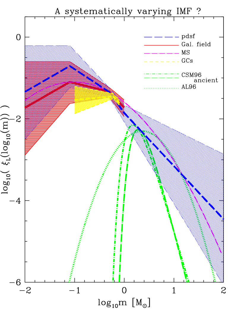
A short account is made of the most promising evidence for a systematically varying IMF. The discussion in Sections 6.3.1 to 6.3.2 is visualised in Fig. 14, in which the various IMFs are compared.

Fig. 14.—: Evidence for a systematically changing IMF. The present-day star-formation (pdsf) IMF (eq. 6) is shown as the thick dashed line. The Galactic-field IMF (eq. 2) is the thick solid line. It is truncated at $m=1\,M_{\odot}$ to express our ignorance about the IMF for $m>1\,M_{\odot}$ for this population that has an average age of about 5 Gyr (the “dichotomy problem”, Section 6.1). In both cases the shaded areas represent the approximate 95–99 per cent confidence region. For comparison, the Miller & Scalo (1979) log-normal IMF for a constant star-formation rate and a Galactic disk age of 12 Gyr is plotted as the thin long-dash-dotted curve (it’s derivative is shown in Fig. 1). Seven globular clusters give $\alpha_{1}=0.89$, with upper and lower values of 1.22 and 0.53, and $\alpha_{2}=2.3$ for $0.6<m<0.8\,M_{\odot}$ (Piotto & Zoccali 1999) as indicated by the short-dashed lines and the heavily shaded area. Three possible IMFs for Galactic-halo WD-progenitors are suggested by the thick long-dash-dotted and short-dash-dotted lines (Chabrier, Segretain & Méra 1996, CSM96), and the thick dotted line (Adams & Laughlin 1996, AL96). The MFs have been scaled such that they agree near $0.5\,M_{\odot}$, except for the ancient IMFs, which are scaled to fit the Galactic-field IMF near $2\,M_{\odot}$.

6.3.1 Globular clusters vs Galactic field

The suggestion in Section 6.2 that the alpha-plot (Fig. 1) may imply a present-day star-formation (pdsf) IMF (eq. 6) that is steeper than the Galactic-field IMF (eq. 2) is interesting when compared to the MFs estimated for globular clusters (Section 6.1). These are very ancient and metal poor systems, so that a systematically different IMF (Larson 1998) ought to be manifest in the data. The difference should be in the sense that globular clusters ought to contain a characteristic stellar mass that is larger than that in more metal-rich populations. The systematically flatter MF in globular clusters compared to the Galactic-field IMF (eq. 2), and especially to the pdsf IMF (eq. 6), may thus be due to a real difference in the star-formation conditions.

However, unfortunately the evidence is not conclusive because globular clusters have lost preferentially low-mass stars, leading to a systematic flattening of the MF with time, unless the clusters are at large Galactocentric distances (Vesperini & Heggie 1997). The binary proportion in globular clusters is typically smaller ($f\mbox{$\,\mathrel{\mathchoice{{\mbox{\lower 2.15277pt\vbox{\halign{$\mathsurround=0pt \displaystyle\hfil#\hfil$\cr<\crcr\sim\crcr}}}}}{{\mbox{\lower 2.15277pt\vbox{\halign{$\mathsurround=0pt \textstyle\hfil#\hfil$\cr<\crcr\sim\crcr}}}}}{{\mbox{\lower 2.15277pt\vbox{\halign{$\mathsurround=0pt \scriptstyle\hfil#\hfil$\cr<\crcr\sim\crcr}}}}}{{\mbox{\lower 2.15277pt\vbox{\halign{$\mathsurround=0pt \scriptscriptstyle\hfil#\hfil$\cr<\crcr\sim\crcr}}}}}}\,$}0.3$) than in the Galactic field ($f\approx 0.6$) but probably not negligible (Hut et al. 1992; Meylan & Heggie 1997), and correction for their effects may also steepen the measured MF. Approximate corrections that increase the measured $\alpha$ are $\Delta\alpha<1$ for dynamical evolution (fig. 6 in Vesperini & Heggie 1997) and $\Delta\alpha\approx 0.2$ for unresolved binary systems, but a case-by-case study is required for detailed estimates. In their sample, Piotto & Zoccali (1999) find evidence for flatter MFs at smaller Galactocentric distances suggesting loss of low-mass stars as being an important bias. But, there is also evidence for a correlation such that more metal-rich clusters have larger $\alpha$.

The Galactic-field IMF (eq. 2) is valid for stars that are, on average, about 5 Gyr old, and which were formed at a different epoch of Galactic evolution than the stars in the clusters featuring in Fig. 1. This, then, suggests a possible systematic shift of star formation towards producing relatively more low-mass stars as star-formation moves towards conditions that may favour lower fragmentation masses through higher metallicities and lower cloud temperatures. That the pre-stellar core MF in $\rho$ Oph is somewhat steeper than the Galactic-field IMF (eq. 2), while being consistent with a fragmentation origin (Motte et al. 1998), supports this notion.

6.3.2 Galactic-halo white dwarfs

Another possible empirical hint for a variable IMF may be provided if part of the dark halo of the Galaxy were in the form of ancient white dwarfs. This is becoming a distinct possibility, given that a handful of candidate ancient halo white dwarfs have been discovered (Elson, Santiago & Gilmore 1996; Ibata et al. 1999, 2000; Méndez & Minniti 2000).

From eq. 2 one obtains per WD progenitor ($1-8\,M_{\odot}$, e.g. Weidemann 1990) about 8 dwarfs with $m=0.1-0.7\,M_{\odot}$. No such halo dwarfs that might belong to the same population as the putative WDs have been found, requiring a radically different IMF for their progenitor stars than is seen today in the Galactic disk. Also, for consistency with chemical enrichment data, such an IMF cannot have many stars with $m\mbox{$\,\mathrel{\mathchoice{{\mbox{\lower 2.15277pt\vbox{\halign{$\mathsurround=0pt \displaystyle\hfil#\hfil$\cr>\crcr\sim\crcr}}}}}{{\mbox{\lower 2.15277pt\vbox{\halign{$\mathsurround=0pt \textstyle\hfil#\hfil$\cr>\crcr\sim\crcr}}}}}{{\mbox{\lower 2.15277pt\vbox{\halign{$\mathsurround=0pt \scriptstyle\hfil#\hfil$\cr>\crcr\sim\crcr}}}}}{{\mbox{\lower 2.15277pt\vbox{\halign{$\mathsurround=0pt \scriptscriptstyle\hfil#\hfil$\cr>\crcr\sim\crcr}}}}}}\,$}5\,M_{\odot}$ (Chabrier, Segretain & Méra 1996; Adams & Laughlin 1996; Larson 1998; Chabrier 1999).

6.3.3 Radial variation in a very young cluster

Hillenbrand (1997) demonstrates that the ONC has pronounced mass segregation, and this may be interpreted as an IMF which has a radial variation, if dynamical mass segregation is not fast enough to produce such mass segregation within the age of the cluster. The age of the ONC is estimated to be less than 1 Myr for most ONC stars (Hillenbrand 1997; Palla & Stahler 1999), and Bonnell & Davies (1998) suggest, by using a softened $N$-body code, that mass segregation takes too long to produce the observed effect. However, stellar-dynamical computations with a direct $N$-body code that correctly treats the many close encounters must be applied to this problem (Kroupa, in preparation). If the mass-segregation time-scale is too long to produce the observed effect, then we would have a well-documented case of a variable IMF most likely through interactions of pre-stellar cores, as suggested by Bonnell et al. (1998) and Klessen (2001).

7 CONCLUSIONS

The following three main points are covered in this paper:

I. The Galactic-field IMF. The form of the average IMF consistent with constraints from local star-count data and Scalo’s (1998) compilation of MF power-law indices for young clusters and OB associations is inferred. The IMF is given by eq. 2. This form may be taken as the universally valid IMF.

II. The alpha-plot: scatter and systematics. Assuming the universal IMF (eq. 2), how large are the apparent variations produced by Poisson noise, the dynamical evolution of star-clusters and unresolved binary systems?

This is studied by making use of the alpha-plot, in which IMF power-law indices inferred for $N$-body model populations are plotted as a function of stellar mass. The extreme assumption is made that the observer can measure each stellar or binary-system mass exactly. The resultant apparent variation of the IMF thus defines the fundamental limit for detecting true variations. Any true variation of the IMF that is smaller than this fundamental limit cannot be detected. This is the reason why no robust evidence for a variable IMF has surfaced to date. The available population samples are too small (e.g. one ONC vs one $\rho$ Oph).

The model clusters have an initial binary proportion of unity and contain $N=800,3000$ and $10^{4}$ stars with a central density as in the ONC. Clusters with a smaller initial density evolve on a longer time-scale. The binary-star problem is thus potentially worse in less-dens clusters, because binary systems survive for longer.

The observed spread of power-law indices is arrived at approximately. For the ensemble of model clusters studied here it is $\sigma_{\alpha}\approx 0.7$ for BDs, $\sigma_{\alpha}\approx 0.5$ for stars in the mass range $0.1-1\,M_{\odot}$, and $\sigma_{\alpha}\approx 1$ for stars with $m\mbox{$\,\mathrel{\mathchoice{{\mbox{\lower 2.15277pt\vbox{\halign{$\mathsurround=0pt \displaystyle\hfil#\hfil$\cr>\crcr\sim\crcr}}}}}{{\mbox{\lower 2.15277pt\vbox{\halign{$\mathsurround=0pt \textstyle\hfil#\hfil$\cr>\crcr\sim\crcr}}}}}{{\mbox{\lower 2.15277pt\vbox{\halign{$\mathsurround=0pt \scriptstyle\hfil#\hfil$\cr>\crcr\sim\crcr}}}}}{{\mbox{\lower 2.15277pt\vbox{\halign{$\mathsurround=0pt \scriptscriptstyle\hfil#\hfil$\cr>\crcr\sim\crcr}}}}}}\,$}1\,M_{\odot}$ (Fig. 13).

For stars with $m\mbox{$\,\mathrel{\mathchoice{{\mbox{\lower 2.15277pt\vbox{\halign{$\mathsurround=0pt \displaystyle\hfil#\hfil$\cr>\crcr\sim\crcr}}}}}{{\mbox{\lower 2.15277pt\vbox{\halign{$\mathsurround=0pt \textstyle\hfil#\hfil$\cr>\crcr\sim\crcr}}}}}{{\mbox{\lower 2.15277pt\vbox{\halign{$\mathsurround=0pt \scriptstyle\hfil#\hfil$\cr>\crcr\sim\crcr}}}}}{{\mbox{\lower 2.15277pt\vbox{\halign{$\mathsurround=0pt \scriptscriptstyle\hfil#\hfil$\cr>\crcr\sim\crcr}}}}}}\,$}1\,M_{\odot}$, the system MF has, on average, the same power-law index as the underlying single-star IMF. That is, the present models do not lead to any systematic bias in this mass range (but see caveat in Section 2.1.1). Similarly, for BDs the input $\alpha$ is arrived at in the mean, but only if the population is at least a few crossing times old, because by then most BD binaries and star–BD binaries have been disrupted. For a dynamically younger population, $\alpha$ (and the number of BDs) will be underestimated depending on the binary proportion.

To correct for unresolved binaries, the measured power-law index has to be increased by $0\mbox{$\,\mathrel{\mathchoice{{\mbox{\lower 2.15277pt\vbox{\halign{$\mathsurround=0pt \displaystyle\hfil#\hfil$\cr<\crcr\sim\crcr}}}}}{{\mbox{\lower 2.15277pt\vbox{\halign{$\mathsurround=0pt \textstyle\hfil#\hfil$\cr<\crcr\sim\crcr}}}}}{{\mbox{\lower 2.15277pt\vbox{\halign{$\mathsurround=0pt \scriptstyle\hfil#\hfil$\cr<\crcr\sim\crcr}}}}}{{\mbox{\lower 2.15277pt\vbox{\halign{$\mathsurround=0pt \scriptscriptstyle\hfil#\hfil$\cr<\crcr\sim\crcr}}}}}}\,$}\Delta\alpha_{0}\mbox{$\,\mathrel{\mathchoice{{\mbox{\lower 2.15277pt\vbox{\halign{$\mathsurround=0pt \displaystyle\hfil#\hfil$\cr<\crcr\sim\crcr}}}}}{{\mbox{\lower 2.15277pt\vbox{\halign{$\mathsurround=0pt \textstyle\hfil#\hfil$\cr<\crcr\sim\crcr}}}}}{{\mbox{\lower 2.15277pt\vbox{\halign{$\mathsurround=0pt \scriptstyle\hfil#\hfil$\cr<\crcr\sim\crcr}}}}}{{\mbox{\lower 2.15277pt\vbox{\halign{$\mathsurround=0pt \scriptscriptstyle\hfil#\hfil$\cr<\crcr\sim\crcr}}}}}}\,$}1.3$ for BDs and $0.5\mbox{$\,\mathrel{\mathchoice{{\mbox{\lower 2.15277pt\vbox{\halign{$\mathsurround=0pt \displaystyle\hfil#\hfil$\cr<\crcr\sim\crcr}}}}}{{\mbox{\lower 2.15277pt\vbox{\halign{$\mathsurround=0pt \textstyle\hfil#\hfil$\cr<\crcr\sim\crcr}}}}}{{\mbox{\lower 2.15277pt\vbox{\halign{$\mathsurround=0pt \scriptstyle\hfil#\hfil$\cr<\crcr\sim\crcr}}}}}{{\mbox{\lower 2.15277pt\vbox{\halign{$\mathsurround=0pt \scriptscriptstyle\hfil#\hfil$\cr<\crcr\sim\crcr}}}}}}\,$}\Delta\alpha_{1,2}\mbox{$\,\mathrel{\mathchoice{{\mbox{\lower 2.15277pt\vbox{\halign{$\mathsurround=0pt \displaystyle\hfil#\hfil$\cr<\crcr\sim\crcr}}}}}{{\mbox{\lower 2.15277pt\vbox{\halign{$\mathsurround=0pt \textstyle\hfil#\hfil$\cr<\crcr\sim\crcr}}}}}{{\mbox{\lower 2.15277pt\vbox{\halign{$\mathsurround=0pt \scriptstyle\hfil#\hfil$\cr<\crcr\sim\crcr}}}}}{{\mbox{\lower 2.15277pt\vbox{\halign{$\mathsurround=0pt \scriptscriptstyle\hfil#\hfil$\cr<\crcr\sim\crcr}}}}}}\,$}0.8$ for $0.08\leq m\leq 1\,M_{\odot}$, the upper and lower limits applying for clusters that are unevolved ($t=0$) and a few crossing times old, respectively, assuming $f=1$ when $t=0$. For a population in a cluster that is a few crossing times old, the corrections reduce to $\Delta\alpha_{0}\approx 0$ and $\Delta\alpha_{1,2}\approx 0.5$. These corrections have to be applied to any young population to infer the single-star IMF.

Finally, as a cautionary remark, the left and right parts of the alpha-plot are observationally disjoint. It is an act of faith to assume that $\alpha(m)$ has the smooth dependence given by eq. 2.

III. IMF variations. Applying the above corrections to the ensemble of observed young clusters, a revised (or present-day star-formation) IMF is arrived at (eq. 6). It is steeper for $m\mbox{$\,\mathrel{\mathchoice{{\mbox{\lower 2.15277pt\vbox{\halign{$\mathsurround=0pt \displaystyle\hfil#\hfil$\cr<\crcr\sim\crcr}}}}}{{\mbox{\lower 2.15277pt\vbox{\halign{$\mathsurround=0pt \textstyle\hfil#\hfil$\cr<\crcr\sim\crcr}}}}}{{\mbox{\lower 2.15277pt\vbox{\halign{$\mathsurround=0pt \scriptstyle\hfil#\hfil$\cr<\crcr\sim\crcr}}}}}{{\mbox{\lower 2.15277pt\vbox{\halign{$\mathsurround=0pt \scriptscriptstyle\hfil#\hfil$\cr<\crcr\sim\crcr}}}}}}\,$}1\,M_{\odot}$ than the Galactic-field IMF (eq. 2), which is a mixture of star-formation events with an average age of about 5 Gyr. The pre-stellar clump mass-spectrum in the present-day star-forming cloud $\rho$ Oph (Motte et al. 1998; Johnstone et al. 2000) also indicates a steeper single-star MF than the Galactic-field MF. Intriguingly, the ancient MFs in globular clusters have $\alpha\mbox{$\,\mathrel{\mathchoice{{\mbox{\lower 2.15277pt\vbox{\halign{$\mathsurround=0pt \displaystyle\hfil#\hfil$\cr>\crcr\sim\crcr}}}}}{{\mbox{\lower 2.15277pt\vbox{\halign{$\mathsurround=0pt \textstyle\hfil#\hfil$\cr>\crcr\sim\crcr}}}}}{{\mbox{\lower 2.15277pt\vbox{\halign{$\mathsurround=0pt \scriptstyle\hfil#\hfil$\cr>\crcr\sim\crcr}}}}}{{\mbox{\lower 2.15277pt\vbox{\halign{$\mathsurround=0pt \scriptscriptstyle\hfil#\hfil$\cr>\crcr\sim\crcr}}}}}}\,$}0$, but closer to 0 than the Galactic-field IMF. The recent detection of candidate white dwarfs in the Galactic halo suggests that the IMF of the progenitor population must have been radically different by producing few if any low-mass and massive stars ($\alpha<<0$ for $m\mbox{$\,\mathrel{\mathchoice{{\mbox{\lower 2.15277pt\vbox{\halign{$\mathsurround=0pt \displaystyle\hfil#\hfil$\cr<\crcr\sim\crcr}}}}}{{\mbox{\lower 2.15277pt\vbox{\halign{$\mathsurround=0pt \textstyle\hfil#\hfil$\cr<\crcr\sim\crcr}}}}}{{\mbox{\lower 2.15277pt\vbox{\halign{$\mathsurround=0pt \scriptstyle\hfil#\hfil$\cr<\crcr\sim\crcr}}}}}{{\mbox{\lower 2.15277pt\vbox{\halign{$\mathsurround=0pt \scriptscriptstyle\hfil#\hfil$\cr<\crcr\sim\crcr}}}}}}\,$}0.5\,M_{\odot}$ and $\alpha>>0$ for $m\mbox{$\,\mathrel{\mathchoice{{\mbox{\lower 2.15277pt\vbox{\halign{$\mathsurround=0pt \displaystyle\hfil#\hfil$\cr>\crcr\sim\crcr}}}}}{{\mbox{\lower 2.15277pt\vbox{\halign{$\mathsurround=0pt \textstyle\hfil#\hfil$\cr>\crcr\sim\crcr}}}}}{{\mbox{\lower 2.15277pt\vbox{\halign{$\mathsurround=0pt \scriptstyle\hfil#\hfil$\cr>\crcr\sim\crcr}}}}}{{\mbox{\lower 2.15277pt\vbox{\halign{$\mathsurround=0pt \scriptscriptstyle\hfil#\hfil$\cr>\crcr\sim\crcr}}}}}}\,$}2\,M_{\odot}$).

Furthermore, the well-developed mass segregation in the very young ($\mbox{$\,\mathrel{\mathchoice{{\mbox{\lower 2.15277pt\vbox{\halign{$\mathsurround=0pt \displaystyle\hfil#\hfil$\cr<\crcr\sim\crcr}}}}}{{\mbox{\lower 2.15277pt\vbox{\halign{$\mathsurround=0pt \textstyle\hfil#\hfil$\cr<\crcr\sim\crcr}}}}}{{\mbox{\lower 2.15277pt\vbox{\halign{$\mathsurround=0pt \scriptstyle\hfil#\hfil$\cr<\crcr\sim\crcr}}}}}{{\mbox{\lower 2.15277pt\vbox{\halign{$\mathsurround=0pt \scriptscriptstyle\hfil#\hfil$\cr<\crcr\sim\crcr}}}}}}\,$}2$ Myr) ONC may exemplify a locally radially-varying IMF, if dynamical mass segregation is too slow. If $N$-body calculations confirm this to be the case (work is in progress), then the ONC will be definite proof that the local conditions determine the average stellar mass, rather than it merely being the result of statistical fluctuations.

The tentative suggestion is thus that some systematic variation may have been detected, with star-formation possibly producing relatively more low-mass stars at later Galactic epochs. Such a variation would be expected in the mass range ($\mbox{$\,\mathrel{\mathchoice{{\mbox{\lower 2.15277pt\vbox{\halign{$\mathsurround=0pt \displaystyle\hfil#\hfil$\cr<\crcr\sim\crcr}}}}}{{\mbox{\lower 2.15277pt\vbox{\halign{$\mathsurround=0pt \textstyle\hfil#\hfil$\cr<\crcr\sim\crcr}}}}}{{\mbox{\lower 2.15277pt\vbox{\halign{$\mathsurround=0pt \scriptstyle\hfil#\hfil$\cr<\crcr\sim\crcr}}}}}{{\mbox{\lower 2.15277pt\vbox{\halign{$\mathsurround=0pt \scriptscriptstyle\hfil#\hfil$\cr<\crcr\sim\crcr}}}}}}\,$}1\,M_{\odot}$) in which turbulent fragmentation, which depends on the cooling rate and thus metal abundance, dominates. Future observations of LMC populations might verify if the IMF has systematically smaller $\alpha$ for $m\mbox{$\,\mathrel{\mathchoice{{\mbox{\lower 2.15277pt\vbox{\halign{$\mathsurround=0pt \displaystyle\hfil#\hfil$\cr<\crcr\sim\crcr}}}}}{{\mbox{\lower 2.15277pt\vbox{\halign{$\mathsurround=0pt \textstyle\hfil#\hfil$\cr<\crcr\sim\crcr}}}}}{{\mbox{\lower 2.15277pt\vbox{\halign{$\mathsurround=0pt \scriptstyle\hfil#\hfil$\cr<\crcr\sim\crcr}}}}}{{\mbox{\lower 2.15277pt\vbox{\halign{$\mathsurround=0pt \scriptscriptstyle\hfil#\hfil$\cr<\crcr\sim\crcr}}}}}}\,$}1\,M_{\odot}$ than the Galactic-field or present-day star-formation IMF. Unfortunately though, even if there is a trend with metallicity, it will be very arduous to uncover a systematic difference in $\alpha$ between the MW and LMC at low masses because the metallicity difference is not very large while the $\alpha$-scatter is. A lack of systematic differences in $\alpha$ for $m\mbox{$\,\mathrel{\mathchoice{{\mbox{\lower 2.15277pt\vbox{\halign{$\mathsurround=0pt \displaystyle\hfil#\hfil$\cr>\crcr\sim\crcr}}}}}{{\mbox{\lower 2.15277pt\vbox{\halign{$\mathsurround=0pt \textstyle\hfil#\hfil$\cr>\crcr\sim\crcr}}}}}{{\mbox{\lower 2.15277pt\vbox{\halign{$\mathsurround=0pt \scriptstyle\hfil#\hfil$\cr>\crcr\sim\crcr}}}}}{{\mbox{\lower 2.15277pt\vbox{\halign{$\mathsurround=0pt \scriptscriptstyle\hfil#\hfil$\cr>\crcr\sim\crcr}}}}}}\,$}10\,M_{\odot}$ between MW and LMC populations may be a result of one physical mechanism, such as coalescence, dominating in the assembly of massive stars (Larson 1999).

Acknowledgements I am grateful to John Scalo for letting me have his compilation of mass function power-law indices, and I thank Sverre Aarseth for making Nbody6 freely available. The calculations were performed at the Institute for Theoretical Astrophysics, Heidelberg University, where I spent a few very pleasant years. I acknowledge support through DFG grant KR1635.

REFERENCES

Aarseth S.J., 1999, PASP, 111, 1333

Aarseth S.J., 2000, Gravitational N-Body Simulations, in prep.

Aarseth S.J., Hénon M., Wielen R., 1974, A&A, 37, 183

Adams F.C., Laughlin G., 1996, ApJ, 468, 586 (AL96)

Allen E.J., Bastien P., 1995, ApJ, 452, 652

Baraffe I., Chabrier G., Allard F., Hauschildt P.H., 1997, A&A, 327, 1054

Bastien P., 1981, A&A, 93, 160

Bonnell I.A., Davies M.B., 1998, MNRAS, 295, 691

Bonnell I.A., Bate M.R., Zinnecker H., 1998, MNRAS, 298, 93

Brandl B., Brandner W., Eisenhauer F., Moffat A.F.J., Palla F., Zinnecker H., 1999, A&A, 352, L69

Briceno C., Hartmann L., Stauffer J., Martin E., 1998, AJ, 115, 2074

Chabrier G., 1999, ApJ, 513, L103

Chabrier G., Baraffe I., 2000, ARA&A, 38, 337 (astro-ph/0006383)

Chabrier G., Segretain L., Méra D., 1996, ApJ, 468, L21

Comeron F., Rieke G.H., Rieke M.J., 1996, ApJ, 473, 294

Dominguez I., Chieffi A., Limongi M., Straniero O., 1999, ApJ, 524, 226

Duchene G., 1999, A&A, 341, 547

Duchene G., Bouvier J., Simon T., 1999, A&A, 343, 831

Duquennoy A. & Mayor M., 1991, A&A, 248, 485

Eisenhauer F., Quirrenbach A., Zinnecker H., Genzel R., 1998, ApJ, 498, 278

Elmegreen B.G., 1999, ApJ, 515, 323

Elson R.A.W., Santiago B.X., Gilmore G.F., 1996, NewA, 1, 1

Evans N.R., 1995, ApJ, 445, 393

Figer D.F., Kim S.S., Morris M., Serabyn E., et al., 1999, ApJ, 525, 750

de La Fuente Marcos R., 1997, A&A, 322, 764

Ghez A.M., McCarthy D.W., Patience J.L., Beck T.L., 1997, ApJ, 481, 378

Gilmore G., Howell D. (eds), 1998, The Stellar Initial Mass Function, San Francisco: ASP

Gilmore G., Perryman M., Lindegren L., Favata F., et al., 1998, in Astronomical Interferometry, ed. R.D. Reasenberg, Proc. SPIE Vol. 3350, p. 541

Gould A., Bahcall J.N., Flynn C., 1997, ApJ, 482, 913

Haywood M., Robin A.C., Crézé M., 1997, A&A, 320, 428

Heger A., Langer N., 2000, ApJ, 544, 1016

Heggie D.C., 1975, MNRAS, 173, 729

Henry T.J., Ianna P.A., Kirkpatrick J.D., Jahreiss H., 1997, AJ, 114, 388

Herbst T.M., Thompson D., Fockenbrock R., Rix H.-W., et al., 1999, ApJ, 526, L17

Hillenbrand L.A., 1997, AJ, 113, 1733

Hillenbrand L.A., Carpenter J.M., 2000, ApJ, 540, 236

Holtzman J.A., Mould J.R., Gallagher III J.S., Watson A.M., et al., 1997, AJ, 113, 656

Holtzman J.A., Watson A.M., Baum W.A., Grillmair C.J., et al., 1998, AJ, 115, 1946

Hurley J.R., Pols O.R., Tout C.A., 2000, MNRAS, 315, 543

Hut P., McMillan S., Goodman J., Mateo M., Phinney E.S., Pryor C., et al., 1992, PASP, 104, 981

Ibata R.A., Richer H.B., Gilliland R.L., Scott D., 1999, ApJ, 524, L95

Ibata R.A., Irwin M., Bienaymé O., Scholz R., Guibert J., 2000, ApJ, 532, L41

Johnstone D., Wilson C.D., Moriarty-Schieven G., Joncas G., et al., 2000, ApJ, in press

Kähler H., 1999, A&A, 346, 67

Kenyon S.J., Hartmann L., 1995, ApJS, 101, 117

Klessen R.S., Burkert A., 2000, ApJS, 128, 287

Klessen R.S., 2001, ApJL, in press

Kroupa P., 1995a, ApJ, 453, 358

Kroupa P., 1995b, MNRAS, 277, 1491

Kroupa P., 1995c, MNRAS, 277, 1507

Kroupa P., 1995d, MNRAS, 277, 1522

Kroupa P., 2000a, NewA, 4, 615

Kroupa P., 2000b, in ASP Conf. Ser. Vol 211, Massive Stellar Clusters, ed. A. Lancon, C. Boily (San Francisco: ASP), p.233 (astro-ph/0001202)

Kroupa P., 2001a, in Deiters S., Spurzem R., eds., STAR2000: Dynamics of Star Clusters and the Milky Way, ASP Conf. Ser., in press (astro-ph/0011328)

Kroupa P., 2001b, in Grebel E., Brandner W., eds., Modes of Star Formation, ASP Conf. Ser., in press (astro-ph/0102155)

Kroupa P., Aarseth S.J., Hurley J.R., 2001, MNRAS, in press

Kroupa P., Tout C.A., 1992, MNRAS, 259, 223

Kroupa P., Tout C.A., Gilmore G., 1991, MNRAS, 251, 293 (KTG91)

Kroupa P., Tout C.A., Gilmore G., 1993, MNRAS, 262, 545 (KTG93)

Kurucz R.L., 2000, in Proceedings of the Workshop on Nearby Stars, in press (astro-ph/0003069)

Lada C.J., Lada E.A., 1991, in: The Formation and Evolution of Star Clusters, ed. James K., ASP Conf. Ser. Vol 13, p.3

Larson R.B., 1998, MNRAS, 301, 569

Larson R.B., 1999, in Star Formation 1999, ed. T. Nakamoto, p. 336 (astro-ph/9908189)

Luhman K.L., 2000, ApJ, 544, 1044

Luhman K.L., Rieke G.H., 1998, ApJ, 497, 354

Luhman K.L., Rieke G.H., 1999, ApJ, 525, 440

Maciel W.J., Rocha-Pinto H.J., 1998, MNRAS, 299, 889

Maeder A., Meynet G., 2000, ARA&A, 38, 143

Martin E.L., Brandner W., Bouvier J., et al., 2000, ApJ, 543, 299

Mason B.D., Gies D.R., Hartkopf W.I., Bagnuolo W.G., et al., 1998, AJ, 115, 821

Massey P., 1998, in ASP Conf. Ser. Vol. 142, The Stellar Initial Mass Function, eds. G. Gilmore & D. Howell (San Francisco: ASP), p.17

Massey P., Hunter D.A., 1998, ApJ, 493, 180

Massey P., Lang C.C., Degioia-Eastwood K., Garmany C.D., 1995a, ApJ, 438, 188

Massey P., Johnson K.E., Degioia-Eastwood K., 1995b, ApJ, 454, 151

McCaughrean M.J., Stauffer J.R., 1994, AJ, 108, 1382

Méndez R.A, Minniti D., 2000, ApJ, 529, 911

Meusinger H., Schilbach E., Souchay J., 1996, A&A, 312, 833

Meylan G., Heggie D.C., 1997, A&AR, 8, 1

Miller G.E., Scalo J.M., 1979, ApJS, 41, 513

Motte F., André P., Neri R., 1998, A&A, 336, 150

Muench A.A., Lada E.A., Lada C.J., 2000, ApJ, 533, 358

Murray S.D., Lin D.N.C., 1996, ApJ, 467, 728

Najita J.R., Tiede G.P., Carr J.S., 2000, ApJ, 541, 977

Palla F., Stahler S.W., 1999, ApJ, 525, 772

Paresce F., De Marchi G., 2000, ApJ, 534, 870

Piotto G., Zoccali M., 1999, A&A, 345, 485

Preibisch T., Balega Yu., Hofmann K.-H., Weigelt G., Zinnecker H., 1999, NewA, 4, 531

Press W.H., Teukolsky S.A., Vetterling W.T., Flannery B.P., 1994, Numerical Recipes (Cambridge University Press)

Price N.M., Podsiadlowski Ph., 1995, MNRAS, 273, 1041

Reid I.N., 1991, AJ, 102, 1428

Reid I.N., Gizis J.E., 1997, AJ, 113, 2246

Reid I.N., Kirkpatrick J.D., Liebert J., Burrows, et al., 1999, ApJ, 521, 613

Rocha-Pinto H.J., Scalo J., Maciel W.J., Flynn C., 2000, A&A, 358, 869

Röser S., 1999, Reviews in Modern Astronomy, 12, 79

Sagar R., Richtler T., 1991, A&A, 250, 324

Salpeter E.E., 1955, ApJ, 121, 161

Scalo J.M., 1986, Fund. Cosmic Ph., 11, 1

Scalo J.M., 1998, in ASP Conf. Ser. Vol. 142, The Stellar Initial Mass Function, eds. G. Gilmore & D. Howell (San Francisco: ASP), p.201

Sirianni, M., Nota, A., Leitherer, C., De Marchi, G., Clampin, M., 2000, ApJ, 533, 203

Terlevich E., 1987, MNRAS, 224, 193

Testi L., Palla F., Natta A., 1999, A&A, 342, 515

Vesperini E., Heggie D.C., 1997, MNRAS, 289, 898

Weidemann V., 1990, ARA&A, 28, 103

Williams D.M., Rieke G.H., Stauffer J.R., 1995a, ApJ, 445, 359

Williams D.M., Comeron F., Rieke G.H., Rieke M.J., 1995b, ApJ, 454, 144

Wuchterl G., Tscharnuter W.M., 2000, A&A, submitted

Zoccali M., Cassisi S., Frogel J.A., Gould A., et al., 2000, ApJ, 530, 418