Variable Iron K$\alpha$ Lines in Seyfert 1 Galaxies

Abstract

We find that variability of the iron K$\alpha$ line is common in Seyfert 1 galaxies. Using data from the ASCA archive for objects that have been observed more than once during the mission, we study the time-averaged spectra from individual observations, thereby probing variability on timescales that range from days to years. Since the statistics of the data do not warrant searches for line variability in terms of a complex physical model, we use a simple Gaussian to model the gross shape of the line, and then use the centroid energy, intensity and equivalent width as robust indicators of changes in the line profile. We find that $\sim$$70\%$ of Seyfert 1s (ten out of fifteen) show variability in at least one of these parameters: the centroid energy, intensity, and equivalent width vary in six, four, and eight sources respectively. Due to the low S/N, limited sampling and time averaging, we consider these results to represent lower limits to the rate of incidence of variability. In most cases changes in the line do not appear to track changes in the continuum. In particular, we find no evidence for variability of the line intensity in NGC 4151, suggesting an origin in a region larger than the putative accretion disk, where most of the iron line has been thought to originate. Mkn 279 is investigated on short timescales. The time-averaged effective line energy (as measured by the Gaussian center energy, which is weighted by emission in the entire line profile) is 6.5 keV in the galaxy rest frame. As the continuum flux increases by $20\%$ in a few hours, the Fe K line responds within $\sim$10,000 seconds, with the effective line energy increasing by 0.22 keV ($\sim$10,500 km s^-1). We also examine the Rosat PSPC spectrum of Mkn 279 but find inconsistencies with ASCA. Problems with the ASCA and Rosat calibration that affect simultaneous spectral fits at low energies are discussed in an appendix.

1 Introduction

Active galactic nuclei (AGN) are thought to be powered by the release of gravitational energy as matter falls onto a supermassive black hole. There is currently much evidence supporting this scenario (e.g., see Collin et al. 2000, Mushotzky, Done & Pounds 1993), but the source of the accreting material and how it makes its way into the center of the galaxy remains uncertain. One important piece of the puzzle is understanding how this material is distributed. The current AGN paradigm invokes an accretion disk that extends from approximately the innermost stable orbit of the black hole out to a few hundredths pc in radius ($10^{4}\;\mathrm{r_{g}}$ for a $10^{8}\;\mathrm{M_{\odot}}$ black hole, where $\mathrm{r_{g}}=GM/c^{2}$ is the gravitational radius.). The inner disk is believed to be surrounded by a much larger structure, a few parsecs across. This structure feeds the inner disk, and serves as the obscuring torus in unification schemes (Antonucci 1993), in which the main difference between Type 2 (narrow-line) and Type 1 (broad-line) objects is due to their orientation with respect to the observer (e.g., Antonucci & Miller 1985; Madejski 1999). The current most advanced telescopes cannot image gas disks smaller than a few hundred pc across and so studying AGN on sub-parsec scales requires spectral techniques. One such technique involves measuring the relationship between emission-line and continuum variability. This technique, referred to as reverberation mapping, allows us to infer the sizes and kinematics of regions that reprocess continuum radiation.

To derive the physical properties of the accretion disk and/or other matter that is in the vicinity of the black hole, X-ray observations are crucial. The proximity of the inner edge of the disk to the black hole exposes it to extreme conditions of temperature, ionization and gravity. This causes it to be X-ray bright, not only in emission but also via reprocessing continuum photons. The most robust feature of X-ray reprocessing is the Fe K$\alpha$ fluorescence line. The light crossing time at the innermost stable orbit around a Schwarzschild black hole is $\sim$3000 M₈ s (where M${}_{8}=\mathrm{M_{BH}}/10^{8}\;\mathrm{M_{\odot}}$). Hence, an Fe K$\alpha$ line produced by the inner disk should respond rapidly to changes in the continuum emission, on timescales as short as a few hours. Emission at 100 $\mathrm{r_{g}}$, on the other hand, can have response times as large as 50,000 s. By studying changes in the line intensity, width and skewness, as well as searching for time lags/leads in the Compton reflection component, we can infer important physical properties of the accreting matter, the central black hole and the size and geometry of the Comptonizing medium responsible for the hard X-ray power law (e.g., Reynolds 2000).

So far, time-resolved spectroscopy of the Fe K$\alpha$ line in AGN is scarce. Of past X-ray missions, only the ASCA satellite has had sufficient energy resolution and observing efficiency at $\sim$6 keV to begin to resolve the iron line profile. Many AGN have been observed with ASCA, but the large ratio of signal to noise that is needed for reliable time-resolved spectroscopy of the line is attained for only a few objects. There are only four Seyfert 1 galaxies for which the data have allowed investigation of short-term variability of the shape of the Fe K$\alpha$ line profile: MCG –6-30-15 (Iwasawa et al. 1996), NGC 7314 (Yaqoob et al. 1996), NGC 3516 (Nandra et al. 1999), and NGC 4051 (Wang et al. 1999b). All show variability on timescales less than 30 ks, but the behavior of the line is complex, with some portions responding to continuum variations and others not. This complex pattern is not easy to understand within the framework of pure reverberation (Reynolds 2000). Complicating things further, the line from the disk may be convolved with emission from further out, making deblending important (Weaver & Reynolds 1998).

The best AGNs in which to study line variability are those for which there is reason to believe that the Fe K$\alpha$ line is dominated by emission from the accretion disk. This is most likely the case for Seyfert 1 galaxies, where the mean line profile shows significant Doppler and gravitational broadening, suggesting a strong contribution from the accretion disk (Nandra et al. 1997; hereafter N97). In this paper, we use ASCA observations of Seyfert 1 galaxies to examine the variability properties of the iron line. Our goal is to determine whether variability is common and what it may tell us about the structure of the central engine.

We begin our discussion with a detailed look at Mrk 279 (§2). In this galaxy, we found that the continuum flux changed significantly halfway through the observation and we were prompted to investigate how the Fe-K line responded to this continuum change. Given the limited statistical quality of the data we were motivated to use the emission-weighted centroid (as modeled by a Gaussian) of the line as one of the primary indicators of variability of the line profile. Realizing that this is a powerful probe of line shape variability for limited signal-to-noise data, we launched a program to look for Fe-K line variability across a sample of Seyfert 1 galaxies, rather than focusing on just the few brightest sources. Our sample is defined as all Seyfert 1s with multiple ASCA observations that have been archived in the HEASARC database as of 1999 August. In §3, we apply this new model to the sample of fifteen Seyferts, which does not include Mrk 279 (because it has only been observed once). For this pilot study, we only consider the time-average spectrum of each observation. A discussion of results follows in §4, and our results are summarized in §5. In the process of investigating the broad-band X-ray spectrum of Mrk 279, we encountered significant discrepancies between the ASCA SIS (solid state spectrometer), GIS (gas imaging spectrometer) and the Rosat PSPC (position sensitive proportional counter). These are discussed in an appendix along with a prescription for correcting some time-dependent effects in the SIS data.

2 Mrk 279

2.1 Observations

Mkn 279 was observed with ASCA on 5 December 1994 with the SIS in 2-CCD mode. Using the most recent calibration, preliminary analysis confirmed the known problem of a discrepancy between the lowest-energy response of SIS1 compared with the other three instruments, so we excluded the SIS1 data below 1 keV from our analysis. The remaining SIS data are obtained in bright mode and times of high background are removed based on the criteria recommended in the ASCA data analysis guide. We include grade 6 photon events in the SIS to improve the ratio of signal to noise at high energies (see e.g., Weaver et al. 1996). Approximately 22 ks of good data are obtained from each SIS and 25 ks from each GIS, resulting in 2–10 keV count rates of 0.95, 0.81, 0.56, and 0.69 counts s^-1 in S0, S1, G2 and G3, respectively.

Mkn 279 was observed with the Rosat PSPC on 1993 October 7 for approximately 10 ks. The processed data are obtained from the HEASARC and the source spectrum is extracted with the ftools software package. Background is accumulated from source-free regions near the target and then subtracted. The Rosat and ASCA spectra are grouped to have $\geq 30$ photons in each energy bin and are modeled separately with the xspec spectral fitting package.

2.2 Temporal Variability

Mrk 279 exhibits X-ray variability on timescales ranging from hours to years. Rapid variability is evinced by the ASCA observation, during which the source varied in amplitude by $\sim$$20\%$ in $\sim$10 ks. Modeling the S0 lightcurve in Figure 1 with a constant yields $\chi^{2}/\nu=3.36$, which rules out a constant source at $\gg 99\%$ confidence.

Pointed X-ray observations of Mrk 279 from 1979 to 1994 indicate long-term source variability of up to a factor of 5 (Figure 2). Throughout this entire period the derived photon index remains fairly stable at a value of $\Gamma=1.9$. The exceptions are measurements from HEAO-1 A2 (parenthesis) and Rosat (brackets). The larger Rosat index may result from a soft “excess” emission component that becomes important below $\sim$0.6 keV (§2.3), while the smaller HEAO-1 A2 index may be caused by Compton reflection that flattens the spectrum above $\sim$7 keV. Upon re-examination, the HEAO-1 data published by Weaver, Arnaud and Mushotzky (1995) are consistent with having an underlying photon index of 2.0 when Compton reflection from a disk with a covering factor of $\Omega=2\pi$ is included in the “A2” spectral model.

2.3 The Time-Averaged ASCA and Rosat PSPC Spectra

We first examine the time-averaged spectrum and discuss in turn the following three energy bands: 0.6–1.0 keV, 1–4 keV, and 0.6–10 keV. At energies of 0.6–1.0 and 1–4 keV, Mkn 279 is bright and featureless, and so we can place stringent limits on the shape of the underlying continuum. The Rosat data show no evidence for absorption exceeding that from our Galaxy and so we fix the absorption at the Galactic value of $\mathrm{N_{H}}\ =1.6\pm 0.3\times 10^{20}$ cm^-2 for all spectral fits (Elvis, Lockman & Wilkes 1989). Fitting the data from 0.6 to 1 keV with a model that consists of an absorbed power law yields a photon index of $2.1\pm 0.1$ ($90\%$ confidence error). Going to higher energies and fitting the same model from 1 to 4 keV yields a similar index of $\Gamma=2.06\pm 0.02$. The equality of spectral slope across the entire 0.6 to 4 keV band indicates no evidence for a spectral upturn below 1 keV in the ASCA spectrum (what otherwise might be called a soft “excess”). Considering the entire energy band, a power law provides a statistically good fit (Table 1, model 1; $\chi^{2}/\nu=923/860$), but significant deviations from the power law shape are evident above $\sim$5 keV (Figure 3).

The iron K$\alpha$ line is clearly detected. Adding a narrow Gaussian to model the line (model 2) yields $\Delta\chi^{2}=57.5$ compared to model 1, which represents a highly significant improvement at $\gg$$99\%$ confidence for the addition of two free parameters. Adding another free parameter by allowing the width of the line to vary (model 3) increases the uncertainty in the line energy, but improves the fit further with $\Delta\chi^{2}=18.8$, again significant at $\gg$$99\%$ confidence. Replacing the Gaussian model with an emission line from a disk around a non-rotating black hole (Schwarzschild metric— Fabian et al. 1989) provides a slightly better overall fit (model 4), but in this case requires the disk to be nearly edge-on. However, we found that this broad, large disk line is actually modeling the high-energy excess in the continuum rather than the sharp, narrow line feature (see Figure 3); such an inclination is unlikely given the unabsorbed nature of the continuum source, unless there is a significant misalignment of the accreting (inner) disk and outer disk or torus. A more compelling reason against an edge-on disk is that it would have great difficulty producing the required, large equivalent width (George & Fabian 1991).

We next examine models that include Compton reflection (Magdziarz & Zdziarski 1995). This choice is physically motivated but has its limitations, because ASCA cannot constrain the reflection spectrum well due to its limited bandpass and high-energy effective area, so the amount of reflection is consequently model-dependent. A model with reflection from neutral material and no iron line (model 5) provides a fit that is comparable to models with a broad Gaussian or a disk line ($\chi^{2}/\nu=849/859$). However, the best fits include both Compton reflection and an iron line (models 6, 7, 8 and 9). Comparing $\chi^{2}$, we see that the data cannot distinguish unambiguously between a narrow and broad line because there is a severe degeneracy between the line width and the reflection normalization $R$ ($\chi^{2}/\nu=825.8/857$ for a narrow Gaussian and 824.3/856 with $\sigma=0.14\pm.14$ keV when the width is a free parameter). If a canonical amount of reflection is assumed ($R=1$ for a disk with $\Omega=2\pi$) then the line is barely resolved with $\sigma\simeq 0.35\pm 0.25$ keV (model 8). Including reflection and then fitting the Fe K$\alpha$ line with an emission feature from a disk around a non-rotating black hole yields a disk inclination of $\sim$$30^{\circ}$ (model 9; Figure 4), as opposed to the large inclination found previously when not including reflection (model 4). The smaller inclination is similar to the mean value for Seyfert 1s (N97), suggesting that the reflection model is a reasonable assumption. Note, however, that this model is statistically indistinguishable from Gaussian models 6 and 7.

The Rosat PSPC and ASCA spectra are not consistent. The agreement between column densities is excellent for the PSPC and SIS0, but the PSPC data require a power law having $\Gamma=2.38$. This index is larger by a factor of $\Delta\Gamma\sim 0.4$ compared to the ASCA index of $\Gamma=2.0$. The difference in the photon indices may result from an ASCA miscalibration, it may be caused by a remaining PSPC calibration error (Iwasawa, Fabian and Nandra 1999; Snowden, Turner & Freyberg 2000) or there may be a separate component that dominates the PSPC spectrum. Apparent steepening below $\sim$0.6 keV could also result from a variable soft X-ray component, since the ASCA and PSPC observations are not simultaneous. Because we cannot determine the true source of the discrepancy, we do not discuss joint PSPC and ASCA fits. The ASCA and Rosat cross-calibration is discussed further in the appendix.

2.4 The High- and Low-State ASCA Spectra

Dividing the ASCA data for Mkn 279 according to the high and low flux states indicated in Figure 1 allows a search for spectral changes on $\sim$10,000 s timescales. There is no evidence for a change in photon index or amount of reflection between the two time-resolved spectra, although we cannot rule out changes in the Compton hump as large as $20\%$. On the other hand, the Fe K line appears to vary, although modeling the entire, broadened profile is difficult and the line width and normalization depend on how the continuum is modeled.

In order to make quantitative statements about the variability of the iron line we have taken steps to determine which ASCA measurements are robust. Because of the limited energy resolution, bandpass and S/N of these data, which make it hard to know the shape of the underlying continuum, it is difficult to quantify the shape of broad spectral features. Such is not the case for narrow features, even between models that include or exclude Compton reflection. Therefore we have chosen a method of using a simple empirical model of a single, unresolved Gaussian ($\sigma=0.05$ keV) to model the Fe K line, with the assumption that the energy of this Gaussian reflects the weighted peak of the line profile. The strength of this method is that it provides us with a single, model-independent parameter that we can trust. Any change in the effective line energy indicates that the line profile is changing. Furthermore, this method enables us to significantly increase the number of sources for which we have some iron line variability information from a few to a sizable sample (§3).

The weakness of this method lies in the fact that we are recording a weighted average of the line profile, not necessarily a real change in the peak energy. Therefore we cannot know how the line changes, i.e., whether the energy changes or whether redshifted emission vanishes leaving a blueshifted peak or whether there are absorption or other effects. However, when an energy shift is measured, we can say with confidence that the line profile has changed.

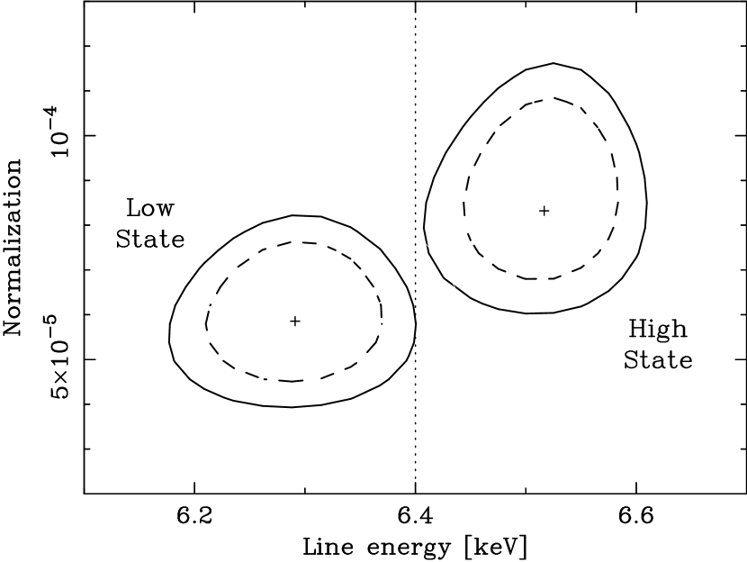
Figure 5: Gaussian line energy vs. normalization for the Fe K$\alpha$ line in the low (left) and high (right) flux states. The dashed and solid contours respectively represent the $68\%$ and $90\%$ confidence levels (for two interesting parameters). The vertical line represents emission from neutral material with no Doppler effects and is drawn as a reference.

For Mkn 279 using a single Gaussian, we find that the effective peak energy of the Fe K$\alpha$ line changes in $\sim$10,000 s by $\sim$$3\%$, increasing from 6.30${}^{+0.10}_{-0.12}$ keV in the low state to 6.52${}^{+0.09}_{-0.09}$ keV in the high state (Figure 5). If interpreted as a simple Doppler shift, this corresponds to a velocity shift of $\sim$10,500 km s^-1. We conclude that there is a significant change in the line profile in $\sim$10,000 s.

3 The ASCA Seyfert 1 Sample

Having established a simple, reliable way to characterize basic variability of the Fe K line profile, we turn to the ASCA sample. This sample is composed of all ASCA observations of all Seyfert 1s with multiple pointings available in the HEASARC public archives as of August 1999, and includes 72 pointings towards 15 galaxies. In an effort to survey this sample for line variability, we apply the approach described for Mkn 279. Unlike our study in §2.4, we limit this initial pilot program to comparisons of the time average spectra of the observations, looking only for variations from one pointing to another. This provides a reliable measure of variability on time scales ranging from days to years, but does not address more rapid changes, such as the $\sim$10 ks variability found in Mkn 279. We leave the study of line variability on intra-observation timescales to future work.

3.1 Spectral Fits

The data are fitted from 1 to 10 keV, using a spectral model consisting of two power laws and a narrow Gaussian. In the galaxy rest frame the spectrum is given by:

$$I=N_{1}E^{-\Gamma}+N_{2}e^{-\mathrm{N_{H}\sigma_{abs}}(E)}E^{-\Gamma}+N_{3}(2\pi\sigma^{2})^{-1/2}e^{-0.5[(E-E_{o})/\sigma]^{2}}\ \mathrm{photons\;s^{-1}\;cm^{-2}\;keV^{-1}}$$

where $\sigma_{\mathrm{abs}}(E)$ is the photoelectric cross-section and $N_{1}$, $N_{2}$, and $N_{3}$ are independent normalizations for each component. When this model is fit to the data, an extra absorbing column at $z=0$ is applied to the entire spectrum. This column density is a free parameter, but is not allowed to be less than the Galactic $\mathrm{N_{H}}$ value. We fix the Gaussian width at $\sigma=50$ eV, which is narrower than the best ASCA spectral resolution in the Fe K region. This representation of the core of the emission line is simply used to characterize the peak energy of the line emission and the flux in the unresolved core of the line. For most galaxies, broadening of the iron line is at best only marginally detectable because of the low signal-to-noise ratio of the data; a narrow Gaussian only grossly underrepresents the ASCA profile for a few cases, such as MCG –6-30-15 (see N97), NGC 4151 (see Yaqoob et al. 1995, Wang, Zhou & Wang 1999a) and NGC 3516 (see Nandra et al. 1999). The continuum model represents an intrinsic underlying power law which intercepts an absorber with a covering fraction equivalent to the ratio of the normalization of the obscured power law to the total continuum normalization. Physically this may either correspond to the source being observed in transmission through a partially covering absorber or the source being observed in transmission through a fully covering absorber but with some fraction of the direct continuum being observed by optically thin reflection out of the line of sight. The signature of such a physical scenario upon a spectrum is illustrated in Figure 6 (left panel). However, a high-energy excess could also be produced by Compton-thick reflection, whereby continuum emission is back-scattered off a Compton thick surface. The signature of Compton-thick reflection is strongest at higher energies (20–50 keV); in the ASCA bandpass it is often difficult to constrain, but it can be parameterized by our second, heavily absorbed power law component. Our model is meant to be a “universal” model that allows us to treat all of the galaxies in our sample identically; it does not require assumptions about the physical nature of the broad, high-energy continuum features. Complex photoelectric absorption is the likely origin of the hard X-ray bump in some targets, such as NGC 4151 (Weaver et al. 1994), while Compton-thick reflection creates the excess in several others, including Mkn 279 (§2). The application of our model to these two extreme cases is illustrated in Figure 6.

Note that the EW values reported here are not necessarily comparable to those reported elsewhere in the literature. They are based upon the observed flux of the line core and the total X-ray continuum, which includes the absorption corrected second power law. The absorption column on the second power law is generally not very well constrained, and can occasionally be quite large. In such cases, the absorption correction can be substantial and hence the EW values can be small. Thus, we consider our relative EW values to be more meaningful than absolute values and therefore focus our discussion upon relative comparisons for the same source. The spectral fits are presented in Table 2.

Spectral results for Seyfert 1 galaxies have been published by Nandra et al. (N97), who presented time-averaged iron line profiles from observations obtained during the first two years of the ASCA mission. To make sure our modeling technique has not introduced spurious effects we compare our results with those of N97, who model the 3–10 keV spectrum with a power law plus a narrow Gaussian and no hard X-ray absorption or reflection. In Figure 8, we compare the distributions of line center energies from N97 with our measurements. Our results are presented in the histogram, with shaded bins denoting observations used by N97. The curves are the best fit Gaussian distributions for the N97 results (dotted curve; $6.34\pm 0.12$ keV), compared with our results for the N97 sample (dashed curve; $6.37\pm 0.09$ keV), and for pointings in either sample (solid curve; $6.38\pm 0.11$ keV; only 64 observations are represented because there was no significant iron line in the other 12). Our measurements compare favorably with the N97 results, both in the mean and individually.

3.2 The Fe K$\alpha$ Line

The emission line and continuum parameters are plotted in Figure 8a–o for all galaxies in our sample. For Fairall 9, NGC 4151, MCG –6-30-15 and NGC 5548, we also show correlation plots of interest in Figure 9a–d.

Of the fifteen galaxies with more than one ASCA pointing, fourteen show significant 2–10 keV variability between observations. Including Mrk 279 (the only Seyfert in which we have looked for intra-observation variability), seven of sixteen galaxies ($\sim$$45\%$) show significant variability of the Fe K$\alpha$ line profile. In $>$$50\%$ we also find variability of the line flux and/or EW. For most cases where we don’t see variability, we are hindered by poor photon counting statistics and sparse sampling. For instance, the four galaxies with only two pointings are also the only four galaxies for which the EW doesn’t vary with at least $68\%$ confidence. If we only consider targets with at least four pointings, we find that six out of nine exhibit variable line energies.

3.3 Results for Individual Galaxies

3.3.1 Fairall 9

This is one of the better-sampled galaxies, with a single 1993 observation followed a year later by a series of seven observations spaced four days apart. The source is variable, with the largest change in 2–10 keV flux ($\sim$$30\%$) occurring in a four day span between the second and third observations (Figure 8a). The error bars are too large to detect a corresponding change in the line flux or EW between these two observations, but there are some general trends when considering the entire data set.

The iron line energy changes significantly (at $99\%$ confidence), with the largest change occurring between observations 7 and 8 (from 6.2 to 6.7 keV), again in a span of four days. For these two pointings, the line energy is lower when the source is fainter, but there is no trend for such behavior when we compare all observations (Figure 9a).

For the line flux and EW we plot both the $68\%$ and $90\%$ confidence error bars in Figure 8a. Neither the line flux nor the EW changes at the $90\%$ confidence level, but they both do with $>68\%$ confidence. There is a hint that the EW is smaller in the higher flux states which would be consistent with a time delay due to a separation between the continuum source and the reprocessing region. If true, this implies a distance of at least 4 light days for the reprocessor.

3.3.2 MCG 8-11-11

Between the two observations of MCG 8-11-11 (taken $<3$ days apart), no change is observed in the 2–10 keV flux, line energy, or line flux (Figure 8b). The low EW reported for the 3 September 1995 observation is a result of a large absorption correction. When we measure the EW without correcting for this absorption, we find a value of $306\pm 84$ eV, which is consistent with that obtained for the other observation.

3.3.3 NGC 3227

The source flux changes by $\sim$$10\%$ between the two ASCA pointings, approximately 2 years apart (Figure 8c). No line variability is observed, but there are only two time-averaged data sets to be compared. We note that during a single observation the continuum changes by as much as a factor of two within a few hours, so there may be interesting variability on time scales that are comparable to Mkn 279. (We have not yet studied in detail the short-timescale behavior of this spectrum).

3.3.4 NGC 3516

NGC 3516 has been observed by ASCA on four occasions. The source flux varies by $\sim$$50\%$, decreasing most between the first and second observations, separated by less than a year (Figure 8d). The line energy changes somewhat on long timescales. Nandra et al. (1999) also find short timescale variability in the line profile.

Changes in line flux and EW are significant. The line flux follows the continuum dropoff between observations 1 and 2 ($\Delta t\simeq 1$ yr), but then increases again as the source becomes fainter ($\Delta t\simeq 3$ yr). This latter change is accompanied by an increase in EW. The fact that the line first follows the continuum change and then becomes stronger as the continuum weakens is difficult to understand in terms of simple disk models of the iron line.

3.3.5 NGC 3783

Among the six observations of this source, the flux is seen to vary by as much as $\sim$$70\%$ (Figure 8e). The line energy changes by $\sim$$3\%$, but there is no clear relationship between line energy and flux, with the line having its highest energies during both low and medium flux states. The statistics are too poor to search for variability in the line flux, but the line EW reaches its largest value during the first observation, when the continuum is weakest.

3.3.6 NGC 4051

The 2–10 keV flux decreases by $\sim$$10\%$ between the two ASCA pointings approximately one year apart (Figure 8f). We do not detect any changes in the iron line between the two observations, but the continuum varies by as much as a factor of $\sim$6 on timescales of a few hours and the short-term variability of the line has been investigated in detail by Wang et al. (1999b). Using a model that consists of a single power law and narrow Gaussian, these authors find that the line profile changes in ways that are independent of the continuum. A very interesting result is that the EW of the Fe K line in NGC 4051 increases as the source brightens (Wang et al. 1999b), as opposed to MCG –6-30-15, where the EW decreases as the source brightens (this paper and Wang et al. 1999b).

3.3.7 NGC 4151

Between the seven ASCA pointings, the 2–10 keV flux varies by as much as $60\%$ (Figure 8g). The line core energy remains constant during this time. The line flux also remains constant, although the error bars are large. Note that for this galaxy we discarded data below 2 keV to mitigate the complexities of the ionized absorber.

Most interesting is the trend for the EW to inversely correlate with the continuum (Figure 9b). The combination of constant line energy, constant flux and decreasing EW with increasing source flux suggests that the line core is dominated by emission far from the black hole. From the time between observations 6 and 7, where the line has not recovered its mean EW, we can place a lower limit of $\sim$1.4 years on the lag in response of the line flux to the continuum, which corresponds to an emission region larger than 0.43 pc ($8.8\times 10^{4}$ M${}_{8}^{-1}\;\mathrm{r_{g}}$). If we use the time scale of the full range of observations, 2.0 years, to define the minimum lag, the emission region is larger than 0.61 pc ($1.3\times 10^{5}$ M${}_{8}^{-1}\;\mathrm{r_{g}}$).

3.3.8 NGC 4593 (Mrk 1330)

The 2–10 keV flux increases by $25\%$ between the two ASCA pointings, approximately 3.5 years apart (Figure 8h). No changes are seen in the iron line between these two observations.

3.3.9 MCG –6-30-15

The 2–10 keV flux varies by $40\%$ between the five ASCA pointings (Figure 8i). Changes in the broad line profile are well documented for this galaxy (e.g., Iwasawa et al. 1996 and Iwasawa et al. 1999). Here, this change is reflected as a change in the effective line energy. We are insensitive to changes in the line on short timescales, but on the longest timescales, we find behavior similar to NGC 4151 in that the line core flux remains fairly constant while the EW decreases with increasing source flux (Figure 9c, lower panel). However, unlike NGC 4151, which has a constant line energy, MCG –6-30-15 has a variable line energy, which suggests that processes are occurring on small spatial scales. The lack of reverberation signatures on long timescales is consistent with the results of Reynolds (2000) and Lee et al. (1998), based primarily on RXTE data.

3.3.10 IC 4329a

This target has been observed on five occasions. The 2–10 keV flux changes by $\sim$$25\%$ (Figure 8j). The line energy changes by less than $4\%$ but the data are not sensitive enough to comment on changes in the EW or line flux.

3.3.11 NGC 5548

The 2–10 keV flux varies by $\sim$$50\%$ (Figure 8k). When the iron line is detected, its energy and flux remain constant. However, the Fe K line is detected in only four of the eight observations. To derive upper limits, we fix the line energy at its mean observed value. In these cases, we find that the line flux and EW has decreased significantly (with $99\%$ confidence), in particular for observation 7 when the source is returning to its bright state. (See line EW vs. continuum correlation in figure 9d).

We have examined whether the disappearance of the line can result from our technique of fitting a narrow Gaussian profile to a line that has become extremely broadened. From a series of fits using a broad Gaussian, both with and without the high-energy power-law component, we find no evidence for a broad line for cases where the narrow line has vanished.

3.3.12 Mrk 841

The 2–10 keV flux increases by $70\%$ between 1994 and 1997 (Figure 8l). The iron line is not detected in the highest flux state (the third of three observations) and the upper limit on the EW is formally inconsistent with the EW in the first observation (with $95\%$ confidence). This is similar to the behavior seen in NGC 5548.

3.3.13 Mrk 509

The 2–10 keV flux changes by as much as a factor of two (Figure 8m). The iron line is detected in only five of eleven observations. When detected, its energy peaks near 6.4 keV, except for observation 10 where the line is detected at 7 keV (6.4 keV is ruled out with $>95\%$ confidence). The statistics are too poor to say much about the line flux and EW, although both are significantly low during the first observation of this galaxy in 1994, as well as in the non-detections of the 2nd and 8th observations.

3.3.14 NGC 7469 (Mrk 1514)

Between the four ASCA pointings, the 2–10 keV flux varies by as much as $50\%$ (Figure 8n). The line energy changes but the errors on line flux and EW are too large to comment more on the variability of these parameters. In a month-long RXTE monitoring campaign, the line flux was found to be well correlated with the 2–10 keV continuum flux, with evidence that the line emitting region lies within a few light days of the continuum source (Nandra et al. 2000).

3.3.15 MCG –2-58-22 (Mrk 926)

MCG –2-58-22 has been observed by ASCA three times. The 2–10 keV flux increases by $100\%$ in 4 years (Figure 8o). The iron line is not detected in the second observation, and the upper limits on the line flux and EW of this observation differ from the other two measurements with $>95\%$ confidence.

4 Discussion

Our Fe K results are summarized in Figure 16. By examining all of the ASCA data for Seyfert 1 galaxies that have multiple pointings available in the archive as of 1999 August, we have shown that variability of the Fe K$\alpha$ line profile on timescales of days to years is common, occurring in at least $40\%$ of the galaxies. We also observe changes in the line flux and/or EW in $\gtrsim 50\%$ of the galaxies. In the one case where we have looked for variability during a single observation (Mkn 279, which has only been observed once by ASCA), we find variability of the line profile on a $\sim$10,000 s timescale.

It is difficult to quantify for an individual galaxy how the changes in the Fe K$\alpha$ line are related to changes in the continuum. This is primarily due to inadequate statistics and poor sampling. However, interesting limits on the reprocessing material and black hole mass can be derived for some cases. Here we examine those limits and discuss various physical mechanisms that may be responsible for producing the observed variability.

4.1 Line Variability in Mrk 279

Mkn 279 possesses an essentially featureless power law continuum, an Fe K$\alpha$ emission line with an equivalent width of $\sim$200 eV that is possibly resolved, and evidence for Compton reflection. Missing are low-energy absorption features such as O VII and O VIII edges that are the signature of a warm absorber (Reynolds 1997), and that are commonly seen in other Seyfert 1s. At low energies the Rosat PSPC spectrum is steeper than the ASCA spectrum by a factor of $\Delta\Gamma\sim 0.4$. This upturn suggests a distinct and possibly variable soft X-ray emission component (see Appendix).

Using a narrow Gaussian to model the core of the Fe K$\alpha$ line, we find evidence for variability in the line profile. As the continuum source increases by an amplitude of $\sim$$20\%$ in 10 ks, the peak energy of the iron line changes by $\sim$$3\%$ ($\sim$10,500 km s^-1; Figure 5). The rapid response of the Fe K$\alpha$ line to the continuum suggests an emission region that is less than a few light-hours across. The light crossing time on a region of the disk with a radius of $x$ in $\mathrm{r_{g}}$ units is $x\;\mathrm{r_{g}}/c\sim 500x\;{\mathrm{M}}_{8}$ s. If we assume the Fe K line is emitted by material in the disk which is orbiting at a distance of at least the marginally stable orbit (in the Schwarzschild metric; $\mathrm{r_{ms}}=6\mathrm{r_{g}}$), this implies a central black hole mass $\lesssim 3\times 10^{8}\;\mathrm{M_{\odot}}$.

4.2 Line Variability in the Seyfert 1 sample

In $40\%$ of Seyfert 1s with multiple ASCA observations, we detect variability of the iron line profile on timescales of days to years, as measured by a change in the effective line peak energy (Figure 16). The detection rate jumps to $67\%$ (6 out of 9) if we only consider the galaxies with better sampling. By examining only the line cores, our measurement represents a lower limit to the variability and will undersample changes in the entire line profile. Variability in the core of the line is interesting however, because the core is expected to be the least variable part of the line if it originates far from the black hole, as is the case in Seyfert 2 galaxies like NGC 2992 (Weaver et al. 1995).

The temporal behavior of the Fe K$\alpha$ line is complex, and sparse sampling hinders our ability to detect any clear variability patterns. The two cases which provide enough information to establish a trend are NGC 4151 and MCG –6-30-15. For NGC 4151, the line flux remains relatively constant on timescales of months to years and does not respond to changes in the continuum. This behavior falls in line with all other historical measurements, which are consistent with a constant line intensity despite large continuum changes. The lag in response of the Fe K line to the continuum suggests that the line originates far from the source of illumination, a conclusion also supported by the fact that the peak energy of the line core stays constant throughout the ASCA observations. Other, more indirect evidence for a partly large emission region is the complex line profile, with a narrow, centrally-peaked component at 6.4 keV superimposed on a broad component (Wang et al. 1999a, Yaqoob et al. 1995). The line properties are thus consistent with simple reverberation models including a non-disk contribution to the emission, possibly from the obscuring torus. BBXRT observed a lack of flux variability in the Fe K line for a 17 hour span, leading to an estimate of $5.8\times 10^{-5}$ pc ($=37\;{\mathrm{M}}_{8}^{-1}\mathrm{r_{g}}$) as the shortest distance from the central source to the region where the line originates (Weaver et al. 1992). ASCA observations have now increased this limit to 2.0 years or 0.61 pc, which corresponds to $1.3\times 10^{5}\;{\mathrm{M}}_{8}^{-1}\mathrm{r_{g}}$.

For MCG –6-30-15, our results show that the line flux remains approximately constant between observations and the EW is inversely proportional to the brightness of the source. However, unlike NGC 4151, the peak energy of the line changes on long timescales (this paper) and short timescales (Iwasawa et al. 1996). The short-term changes in the line profile imply a small emission region. The temporal/spectral behavior of the line is difficult to reconcile with simple models of an accretion disk that produces the Fe K emission from regions close to the black hole. The light crossing time of the inner disk is short compared to the timescales of variability we have examined for sources in the sample, yet we do not generally observe the line flux to respond to the continuum variability as expected. Whether the X-ray source is situated at a central location above the accretion disk (the so-called “lamppost model”, e.g. Nayakshin & Kallman 2000) or in the form of a hot corona on the disk surface (the so-called “sandwich model”, e.g. Collin et al. 2000), one would expect the line flux to track the continuum, yielding a constant equivalent width over the time scales studied, as well as possible changes in the line profile. On the other hand, for a region as large as the outer disk or torus, the light crossing time would be greater than the temporal resolution of the data, in which case we expect the line flux to lag the continuum and we don’t expect changes in the line profile. Obviously, the Fe K line, with it’s variable profile and constant flux, does not easily fit either scenario.

Other objects in our sample possess unusual behavior. In NGC 3516, the line seems to vary independently of the continuum, with the flux dropping with the continuum over the span of a year but then appearing to strengthen again as the continuum drops further in a three-year span. Similar behavior occurs for this galaxy on short timescales (Nandra et al. 1999). In NGC 5548, the line is undetected in half of the observations with fairly strict upper limits, but whether or not the line is present does not seem to relate to the continuum flux state. For Mkn 509, the Fe K line energy increases to $\sim$7 keV during one observation, but this increase does not appear to be related to a change in the continuum.

For the lamppost model, changes in line energy can be explained by changes in the ionization of the disk for different flux states. However, the behavior of the line profile appears to bear little relation to the continuum in general, and so there must be something else responsible for controlling the line shape and/or intensity. One possibility is a physical change in the reprocessor. If the geometry of the accretion disk changes, with the disk extending farther toward the black hole in certain flux states, for example, then this could result in enhanced Doppler shifts resulting in a more significant Doppler-boosted peak and redshifted wing. Another possibility is some kind of time-variable, non-axisymmetric obscuration (Weaver & Yaqoob 1998), which can remove photons in the line core, shifting the mean energy. On the other hand, short-term changes could result from localized flaring phenomena, such that the X-ray illumination is spread over the disk surface unevenly (Nayakshin & Kallman 2000) and most of the X-ray reprocessing happens near the flare locations (e.g., the rotating hot-spot model; Ruszkowski 2000).

Observations with XMM and Constellation-X will be crucial to understand the variability patterns of the iron K lines. However, even with very high-quality data, interpreting time-resolved spectra will require assumptions regarding the accretion disk structure, disk instabilities, diffusion rates, and disk winds and shocks. A roadmap for understanding these types of observations already exists in other disciplines such as studying disk emission in galactic microquasars (Markwardt, Swank & Taam 1999; Eikenberry et al. 1998), but such techniques have yet to be applied to the large accreting systems in active galaxies. It will be important to see if it is possible to relate changes in the lines to specific changes in ionization state, changes in illumination, or changes in disk structure. It may be difficult to distinguish between basic Doppler, gravitational, and ionization effects, and the movement of localized X-ray/UV hot spots until we can image the accretion disk in X-rays.

5 Summary and Conclusions

We have studied variability of the Fe K$\alpha$ line on short time scales in one source, and on longer time scales in a sample of Seyfert 1 galaxies. In the ASCA observation of Mkn 279 we saw a $20\%$ increase in 2–10 keV flux over $\sim$10 ks. In this time, the energy of the Fe K$\alpha$ line core increases from 6.30${}^{+0.10}_{-0.12}$ keV in the low state to 6.52${}^{+0.09}_{-0.09}$ keV in the high state.

The procedure developed for Mkn 279 has allowed us to study the line variability across an entire sample of Seyfert galaxies. By examining the time-averaged data for the 15 Seyfert 1 galaxies with multiple ASCA pointings, we find that variability of the Fe K$\alpha$ line profile is common, appearing in $40\%$ of the objects, and in two thirds of those galaxies which have been observed at least four times. Variability in the line flux and/or EW occur in $\sim$$50\%$ of the galaxies. Because we have examined only the time averages of the line cores, and also due to the limited sampling, our measurements represent a lower limit to the true variability of the line.

The general behavior of the line across the sample bears little relation to the continuum. The data clearly show that in no galaxy does the Fe K$\alpha$ line simply track the continuum. Beyond this, limited sampling makes it difficult to quantify how changes in the Fe K$\alpha$ line are related to changes in the continuum for most galaxies. In NGC 4151 the line core appears to be constant, independent of continuum changes on time scales up to two years; for other Seyfert 1s the Fe line behavior is more complex, and is generally difficult to explain in the context of our current theoretical models. Taken as a whole, we have confirmed with the largest line variability study to date that the simple disk model is inadequate to explain the data. We need to reexamine the assumptions of our models from a theoretical perspective in order to refine them and make them consistent with observations.

Appendix A Appendix: Concerns Regarding ASCA Calibration

There have been ongoing discussions about calibration issues involving the SIS detector response at low energies ($<1$ keV). These calibration problems are especially noticeable when attempting joint spectral analysis with the Rosat PSPC. Part of the problem with joint fits appears to lie with the PSPC, which is known to have temporally-dependent energy nonlinearity and residual, temporally-dependent spatial gain variations (Snowden, Turner & Freyberg 2000). However, part of the problem also stems from the fact that the SIS calibration has not kept pace with the in-flight instrument degradation. There is evidence that the SIS detector response has been degrading steadily since launch, not only in energy resolution but also in loss of effective area at low energies due to the time-dependent effects of radiation damage.

Current software does not account for all of these changes. One example of discrepant results in the literature is a study of X-ray bright galaxy groups by Hwang et al. (1999). Comparing ASCA and the PSPC, these authors find differences between the thermal temperatures and column densities in the sense that the SIS temperatures are systematically lower than the PSPC temperatures and the SIS column densities are systematically higher than the PSPC column densities (the latter tend to agree with Galactic values, as expected). Another example is the Seyfert galaxy NGC 5548, for which simultaneous Rosat and ASCA observations are available. For this galaxy, Iwasawa, Fabian and Nandra (1999) find a clear and unexplained mismatch of photon indices ($\Delta\Gamma\simeq 0.4$) between the SIS and the PSPC. We cite Mkn 279 as another example. The ASCA photon index is significantly less than the PSPC index ($\Delta\Gamma\simeq 0.4$) and the SIS1 column density is significantly larger than the PSPC column density.

In this appendix we examine the nature of the SIS calibration problem, estimate its magnitude and suggest ways to cope with it at the analysis stage. We attempt to explain the ASCA SIS quantum efficiency (“QE”) problem in a self-consistent manner without relying on cross-measurements with Rosat. As we have already stated, the miscalibration between ASCA and Rosat is not totally due to ASCA, but the ASCA problem needs to be quantified.

There are a number of ways to examine the calibration; some being more model-dependent than others. A rigorous and model-independent approach based on examining the ratio of data from the various detectors is followed by Yaqoob in a recent calibration memo (Yaqoob et al. 2000). Our method is based on model fitting, but its strength lies in using the GIS as a cross-calibrator for the SIS. We find that the GIS is sensitive enough to test for small differences in $\mathrm{N_{H}}$ on the order of a few $\times 10^{20}\;\mathrm{cm}^{-2}$, although the absolute calibration is not as accurate as this.

A.1 Cross-calibration of the SIS0 and SIS1

Very briefly, the ASCA detectors were calibrated along the following lines. The GIS was calibrated using the Crab, which is too bright for the SIS. Therefore, the SIS had to calibrated against the GIS. SIS data for the quasar 3C 273 between 2–6 keV were then used to adjust the depletion depth of the SIS model to obtain agreement with GIS data for the same target. The final adjustment of the QE curve for the SIS was released in 1994 November (version 0.8 of sisrmg and the response matrices), and was based on an observation of 3C 273 taken on 16 December 1993. At this point the QE was adjusted again relative to the ground calibration to force consistency between the four ASCA instruments. At the time, it was not realized that the discrepancy that was being corrected was changing with time and so the baseline QE has become out of date. Since then, the response matrix generator has changed in substance only to model certain energy-resolution changes in the detectors.

The degradation of the SIS detectors due to the on-orbit effects of radiation damage on the CCDs shows up as an increasing loss of photons below 1 keV with time. This is manifestly different from the so-called “RDD” (Residual Dark current Distribution) problem (even then, RDD correction software only mitigates some of the RDD problems). The reasons for the additional losses are not understood by the calibration teams. It is suspected that it is due to increasing dark current and loss of Charge Transfer Efficiency (CTE). The problem is still under investigation by the instrument teams. The current trend is more pronounced in S1 than S0 and shows up in 1, 2, and 4 CCD mode data. The absolute magnitude of the effect is larger for modes using a larger number of CCDs but curiously, the ratio of the loss of efficiency seems to be independent of CCD mode (Yaqoob et al. 2000).

The loss in SIS detector efficiency can be parameterized crudely as excess absorption. So, when using the current calibration, observations made before 16 December 1993 have SIS data which appear to turn up at low energies (a negative “absorption”) while observations made after 16 December 1993 have SIS data which appear to turn down at low energies (a positive “absorption,” which has increased with time). December 16 1993 can therefore be viewed as an anchor point at which the time-dependent correction investigated by us and by Yaqoob et al. (2000) is zero.

Adopting the “excess-$\mathrm{N_{H}}$” approach, we illustrate the effect by first showing the magnitude of the effect for the ASCA observation of Mrk 279 taken in December 1994. Mrk 279 is an excellent target to search for charge loss due to its naturally small absorbing column. Then we compare the SIS and GIS data for a sample of AGN that were observed multiple times throughout the mission to attempt a crude cross-calibration.

Mrk 279

This galaxy has no intrinsic absorption according to the PSPC and a fairly low Galactic column density, which makes it an excellent target for soft X-ray calibration. From joint fits with the ASCA PSPC data, we have already noted that the photon indices do not match, but here we compare the column densities. For a power-law model including a low-temperature thermal component to model the steeper Rosat spectrum, we find that the PSPC and S0 measure the same Galactic column density to within statistical uncertainties (Figure 17). However, for the same model for S1, $\mathrm{N_{H}}$(S1) is larger by about $3\times 10^{20}$ cm^-2 (for the same photon index). The consistency of column densities between S0 and the PSPC agrees with the overall trend with time. Mrk 279 was observed early in the mission at a point when S0 had not degraded appreciably while S1 had begun to degrade.

The SIS and GIS

Taking advantage of Seyfert 1 galaxies as cross-calibration sources and comparing the SIS against the GIS, we examine trends for changes in the apparent column density for observations taken in 1-CCD and 2-CCD mode. We fit the data from 0.6 to 4 keV, forcing all of the model parameters to be the same except for the column density. $\mathrm{N_{H}}$ is set to be equal for the two GIS spectra but allowed to be a free parameter for S0 and S1 independently. Our results are summarized in Figure 18. For S0, we see a systematic trend for $\mathrm{N_{H}}$(S0) to increase approximately linearly with time since launch, from $\sim$$2\times 10^{20}$ cm^-2 in 1995 to $\sim$$6\times 10^{20}$ in 1998. The S0 data fit very well with a straight line described by

$$\mathrm{N_{H}}\mathrm{(SIS0)}=3.635857\times 10^{-8}(T-3.017482\times 10^{7})\times 10^{20}\;\mathrm{cm}^{-2}$$

where $T$ is ASCATIME (average of the start and stop times of the observation) in seconds since 1 January 1993.

S1 behaves differently from S0. The trend is not linear, but peaks at around 1500 days since launch. The S1/S0 discrepancy therefore shows no clear trend with time. To “correct” for the change in S1, one could measure the ratio of S1/S0 for a given observation, determine the excess NH(S1/S0),and then add this to NH(S0). If the signal-to-noise is not good enough to measure the S1/S0 ratio then one should not be concerned about correcting the data since statistical errors will dominate over systematic errors.

We note that the GIS has an effect below 1 keV that mimics a negative absorption of $\sim$$2\times 10^{20}$ cm^-2 (the opposite of the SIS). The root cause for this discrepancy seems to be that the soft X-ray GIS and SIS responses were originally calibrated independently. The GIS/XRT response was tuned to the Crab to give a column density of $3\times 10^{21}$ cm^-2 while the SIS low-energy efficiency was only calibrated on the ground. The column density assumed for the Crab carries a larger uncertainty than $2\times 10^{20}$ cm^-2 so the GIS calibration was not intended to be good enough to measure absolute absorption to this level. However, we believe that the GIS detectors are sensitive to differences of this order of column density, so although they can’t be used to make absolute measurements of small column densities, they can measure a small relative difference in $\mathrm{N_{H}}$ compared to the SIS.

The problem with the low-energy inflight calibration of the SIS is that there is no suitable astrophysical source. The ideal requirement is that such a source should be bright, have constant intensity, low intrinsic absorption, a simple continuum, and it should be a point source. No such source exists. 3C 273 is a bright point source but it is variable in both intensity and spectral shape. There are also remaining known problems with the GIS, most importantly uncertainty in the energy to pulse-height relation and this problem is currently being addressed by the instrument teams. This will affect the energy scale and have minor effects on the spectral response. There will also be refinements in the Beryllium window transmission which may affect absolute column density measurements.

The excess-$\mathrm{N_{H}}$ problem affects joint model fits of the PSPC and ASCA if left uncorrected. A global correction of S0 based on Figure 18 may be adequate for sources with simple spectra and moderate count rates, depending on science goals. For high resolution, high-quality spectra of complex line-emitting plasmas this “correction” must be applied with caution because we do not understand the detailed changes of the effective area with energy and it does not model any changes in energy resolution.

Additional effects?

For Mkn 279, the ASCA photon index is smaller than the PSPC index even when we restrict the ASCA fits to energies above 1 keV, where ASCA is well calibrated. So, is there a slope problem different from the low-energy ‘cutoff’ problem? To determine the magnitude of any additional error, we have examined PSPC and ASCA data for MCG –2-58-22, another bright Seyfert 1 galaxy with no intrinsic absorption that was observed early in the mission (Weaver et al. 1995). Including the ‘$\mathrm{N_{H}}$ correction’ for MCG –2-58-22, we find that the PSPC and ASCA indices differ by less than $\Delta\Gamma\sim 0.1$. This remaining slope offset is small enough to suggest that the large slope offset for Mkn 279 is real, at least in this case.

Table 1: ASCA Time-Averaged Spectral Results for Mkn 279

Model	$\Gamma$	E${}_{\rm Fe~{}K\alpha}$	$\sigma_{\rm Fe~{}K\alpha}$	EW${}_{\rm Fe~{}K\alpha}$	$\theta$	$R$	$\chi^{2}/dof$
		[keV]	[keV]	[eV]	[∘]
1) PL	$2.01^{+0.01}_{-0.01}$	$\cdot\cdot\cdot$	$\cdot\cdot\cdot$	$\cdot\cdot\cdot$	$\cdot\cdot\cdot$	$\cdot\cdot\cdot$	922.9/860
2) PL+Gn	$2.02^{+0.01}_{-0.01}$	$6.47^{+0.05}_{-0.06}$	0.01(f)	$196^{+42}_{-42}$	$\cdot\cdot\cdot$	$\cdot\cdot\cdot$	865.4/858
3) PL+Gb	$2.04^{+0.03}_{-0.03}$	$6.50^{+0.12}_{-0.17}$	$0.51^{+1.39}_{-0.27}$	$440^{+90}_{-80}$	$\cdot\cdot\cdot$	$\cdot\cdot\cdot$	846.6/857
4) PL+Dl	$2.03^{+0.02}_{-0.02}$	$6.50^{+0.08}_{-0.08}$	$\cdot\cdot\cdot$	$560^{+80}_{-80}$	$89_{-55}^{*}$	$\cdot\cdot\cdot$	841.1/857
5) PL+R	$2.11^{+0.03}_{-0.03}$	$\cdot\cdot\cdot$	$\cdot\cdot\cdot$	$\cdot\cdot\cdot$	30(f)	$2.54^{+0.63}_{-0.57}$	848.5/859
6) PL+Gn+R	$2.10^{+0.02}_{-0.02}$	$6.47^{+0.07}_{-0.07}$	.01(f)	$120^{+45}_{-45}$	30(f)	$1.91^{+0.62}_{-0.58}$	825.8/857
7) PL+Gb+R	$2.10^{+0.02}_{-0.02}$	$6.46^{+0.09}_{-0.09}$	$0.14^{+0.14}_{-0.14}$	$148^{+68}_{-68}$	30(f)	$1.60^{+0.50}_{-0.62}$	824.3/856
8) PL+Gb+R	$2.06^{+0.02}_{-0.02}$	$6.46^{+0.09}_{-0.09}$	$0.21^{+0.19}_{-0.11}$	$213^{+65}_{-65}$	30(f)	1.0(f)	829.8/857
9) PL+Dl+R	$2.09^{+0.02}_{-0.02}$	$6.46^{+0.10}_{-0.10}$	$\cdot\cdot\cdot$	$210^{+70}_{-70}$	$15_{-15}^{+35}$	$1.50^{+0.44}_{-0.53}$	825.9/856

Note. — Includes grade 6 photon events from the SIS. Fixed parameters are labeled by (f). All models include absorption by the Galaxy ($\mathrm{N_{H}}\ =1.64\times 10^{20}$ cm^-2). Data are fitted from 1 to 10 keV. Errors represent $90\%$ significance. The columns are: (1) model label and description, (2) photon index, (3) rest frame line energy, (4) line width, (5) line equivalent width, (6) inclination of the accretion disk, (7) reflection normalization, and (8) fit quality.

Table 2: Line Properties for a Narrow Gaussian

Galaxy	sequence	Date	CCD	Time	$\mathrm{E_{K\alpha}}$	$\mathrm{N_{K\alpha}}$	$\mathrm{EW_{K\alpha}}$	$\Delta\chi^{2}$	$\mathrm{F_{2-10}}$
			mode	[ks]	[keV]	[$10^{-5}$]	[eV]		[$\times 10^{-12}$]
Fairall 9	71027000	21 Nov 93	1	22.0	$6.32^{+0.07}_{-0.07}$	$\phantom{1}3.1^{+0.9}_{-0.9}$	$120^{+36}_{-35}$	126	$22.0^{+0.8}_{-0.9}$
Fairall 9	73011000	12 Dec 94	1	16.9	$6.33^{+0.08}_{-0.09}$	$\phantom{1}3.1^{+1.3}_{-1.3}$	$\phantom{1}92^{+40}_{-40}$	112	$27.8^{+1.1}_{-1.3}$
Fairall 9	73011010	16 Dec 94	1	15.2	$6.52^{+0.12}_{-0.13}$	$\phantom{1}3.1^{+1.3}_{-1.3}$	$128^{+55}_{-55}$	119	$21.5^{+1.3}_{-1.1}$
Fairall 9	73011020	10 Dec 94	1	18.3	$6.47^{+0.11}_{-0.09}$	$\phantom{1}4.4^{+1.3}_{-1.3}$	$171^{+51}_{-50}$	125	$24.7^{+1.1}_{-1.1}$
Fairall 9	73011030	14 Dec 94	1	18.1	$6.35^{+0.09}_{-0.10}$	$\phantom{1}2.9^{+1.3}_{-1.3}$	$\phantom{1}85^{+38}_{-38}$	111	$24.6^{+1.2}_{-1.0}$
Fairall 9	73011040	18 Dec 94	1	21.4	$6.35^{+0.08}_{-0.08}$	$\phantom{1}3.8^{+1.2}_{-1.2}$	$122^{+39}_{-39}$	121	$27.6^{+1.0}_{-1.2}$
Fairall 9	73011060	22 Dec 94	1	16.4	$6.65^{+0.12}_{-0.15}$	$\phantom{1}2.6^{+1.4}_{-1.4}$	$\phantom{1}84^{+47}_{-47}$	116	$26.1^{+1.1}_{-1.3}$
Fairall 9	73011050	26 Dec 94	1	7.38	$6.20^{+0.09}_{-0.10}$	$\phantom{1}4.1^{+1.7}_{-1.7}$	$158^{+67}_{-66}$	112	$22.3^{+1.4}_{-1.5}$
MCG 8-11-11	73052000	13 Sep 95	1	11.5	$6.45^{+0.05}_{-0.06}$	$\phantom{1}7.2^{+2.0}_{-2.0}$	$7.4^{+2.1}_{-2.1}$	123	$26.9^{+1.7}_{-1.5}$
MCG 8-11-11	73052010	16 Sep 95	1	11.0	$6.45^{+0.09}_{-0.07}$	$\phantom{1}6.0^{+2.1}_{-2.1}$	$179^{+63}_{-63}$	117	$25.3^{+1.8}_{-1.5}$
NGC 3227	70013000	18 May 93	4	36.4	$6.42^{+0.04}_{-0.04}$	$\phantom{1}4.7^{+1.0}_{-1.0}$	$127^{+27}_{-27}$	148	$35.8^{+1.0}_{-1.0}$
NGC 3227	73068000	15 May 95	1	35.8	$6.36^{+0.07}_{-0.07}$	$\phantom{1}5.7^{+1.2}_{-1.2}$	$146^{+30}_{-29}$	162	$31.5^{+1.1}_{-1.1}$
NGC 3516	71007000	12 Apr 94	1	30.1	$6.40^{+0.04}_{-0.04}$	$11.0^{+1.8}_{-1.8}$	$122^{+20}_{-20}$	195	$86.5^{+1.6}_{-1.6}$
NGC 3516	73066000	11 Mar 95	1	19.9	$6.38^{+0.06}_{-0.07}$	$\phantom{1}5.6^{+1.8}_{-1.8}$	$\phantom{1}94^{+29}_{-29}$	123	$54.5^{+1.6}_{-1.6}$
NGC 3516	73066010	12 Mar 95	1	19.0	$6.33^{+0.06}_{-0.06}$	$\phantom{1}7.4^{+1.8}_{-1.8}$	$124^{+30}_{-29}$	140	$54.0^{+1.6}_{-1.5}$
NGC 3516	76028000	12 Apr 98	1	153.	$6.33^{+0.02}_{-0.02}$	$\phantom{1}8.5^{+0.7}_{-0.7}$	$149^{+11}_{-12}$	396	$47.6^{+0.6}_{-0.6}$
NGC 3783	71041000	19 Dec 93	2	17.5	$6.39^{+0.04}_{-0.04}$	$10.4^{+2.0}_{-2.0}$	$164^{+32}_{-32}$	167	$50.0^{+1.7}_{-1.7}$
NGC 3783	71041010	23 Dec 93	2	16.2	$6.24^{+0.07}_{-0.06}$	$\phantom{1}7.6^{+2.3}_{-2.3}$	$\phantom{1}95^{+29}_{-28}$	129	$66.3^{+2.1}_{-2.0}$
NGC 3783	74054000	19 Jul 96	1	17.6	$6.26^{+0.07}_{-0.08}$	$\phantom{1}8.5^{+2.5}_{-2.5}$	$\phantom{1}88^{+26}_{-26}$	130	$85.8^{+2.3}_{-2.2}$
NGC 3783	74054010	11 Jul 96	1	20.4	$6.34^{+0.07}_{-0.07}$	$\phantom{1}8.1^{+2.3}_{-2.3}$	$\phantom{1}93^{+27}_{-27}$	130	$78.0^{+2.0}_{-2.0}$
NGC 3783	74054020	14 Jul 96	1	18.0	$6.35^{+0.06}_{-0.06}$	$10.3^{+2.5}_{-2.5}$	$117^{+29}_{-28}$	142	$82.8^{+2.2}_{-2.2}$
NGC 3783	74054030	16 Jul 96	1	17.7	$6.38^{+0.04}_{-0.04}$	$10.8^{+2.5}_{-2.5}$	$124^{+30}_{-29}$	145	$77.9^{+2.2}_{-2.1}$
NGC 4051	70001000	25 Apr 93	4	27.2	$6.43^{+0.06}_{-0.06}$	$\phantom{1}3.5^{+1.0}_{-1.0}$	$134^{+39}_{-39}$	127	$27.7^{+0.9}_{-0.9}$
NGC 4051	72001000	17 Jun 94	1	72.0	$6.38^{+0.05}_{-0.05}$	$\phantom{1}2.7^{+0.6}_{-0.6}$	$100^{+24}_{-24}$	141	$25.6^{+0.5}_{-0.6}$
NGC 4151	70000000	24 May 93	4	13.6	$6.38^{+0.03}_{-0.03}$	$37.2^{+5.0}_{-5.0}$	$108^{+15}_{-14}$	122	$167.^{+6.}_{-6.}$
NGC 4151	70000010	15 Nov 93	1	7.26	$6.35^{+0.04}_{-0.04}$	$31.4^{+7.1}_{-7.1}$	$\phantom{1}73^{+16}_{-16}$	139	$222.^{+6.}_{-5.}$
NGC 4151	71019030	14 Dec 93	2	11.6	$6.35^{+0.04}_{-0.04}$	$33.7^{+6.5}_{-6.5}$	$\phantom{1}72^{+14}_{-14}$	161	$263.^{+7.}_{-6.}$
NGC 4151	71019020	15 Dec 93	2	10.9	$6.36^{+0.04}_{-0.04}$	$32.3^{+6.4}_{-6.4}$	$\phantom{1}76^{+15}_{-15}$	156	$232.^{+6.}_{-6.}$
NGC 4151	71019010	17 Dec 93	2	12.4	$6.38^{+0.03}_{-0.02}$	$35.3^{+6.3}_{-6.3}$	$\phantom{1}77^{+14}_{-14}$	171	$268.^{+6.}_{-6.}$
NGC 4151	71019000	19 Dec 93	2	12.2	$6.36^{+0.03}_{-0.03}$	$39.0^{+6.1}_{-6.1}$	$\phantom{1}90^{+14}_{-14}$	188	$255.^{+6.}_{-6.}$
NGC 4151	73019000	10 May 95	1	96.8	$6.37^{+0.01}_{-0.01}$	$35.7^{+1.9}_{-1.9}$	$101^{+5}_{-5}$	777	$180.^{+2.}_{-2.}$
NGC 4593	71024000	19 Jan 94	1	22.1	$6.33^{+0.08}_{-0.07}$	$\phantom{1}3.7^{+1.3}_{-1.3}$	$\phantom{1}70^{+25}_{-25}$	117	$40.4^{+1.0}_{-1.3}$
NGC 4593	75023010	20 Jul 97	1	14.0	$6.39^{+0.08}_{-0.08}$	$\phantom{1}5.2^{+2.1}_{-2.1}$	$\phantom{1}83^{+34}_{-34}$	105	$50.8^{+1.8}_{-1.7}$
MCG –6-30-15	70016000	19 Jul 93	2	30.7	$6.27^{+0.07}_{-0.07}$	$\phantom{1}3.3^{+1.3}_{-1.3}$	$\phantom{1}58^{+23}_{-23}$	114	$52.0^{+1.3}_{-1.2}$
MCG –6-30-15	70016010	31 Jul 93	1	29.3	$6.40^{+0.05}_{-0.05}$	$\phantom{1}4.4^{+1.3}_{-1.3}$	$102^{+31}_{-31}$	127	$42.6^{+1.2}_{-1.2}$
MCG –6-30-15	72013000	23 Jul 94	1	161.	$6.42^{+0.05}_{-0.05}$	$\phantom{1}3.9^{+0.6}_{-0.6}$	$\phantom{1}78^{+11}_{-11}$	110	$50.3^{+0.6}_{-0.5}$
MCG –6-30-15	75006000	13 Aug 97	1	85.1	$6.42^{+0.07}_{-0.07}$	$\phantom{1}3.2^{+0.7}_{-0.7}$	$\phantom{1}83^{+20}_{-19}$	145	$39.9^{+0.7}_{-0.6}$
MCG –6-30-15	75006010	17 Aug 97	1	85.8	$6.34^{+0.05}_{-0.05}$	$\phantom{1}4.6^{+0.7}_{-0.7}$	$121^{+19}_{-19}$	194	$37.3^{+0.6}_{-0.6}$
IC 4329a	70005000	15 Aug 93	4	32.1	$6.37^{+0.05}_{-0.05}$	$\phantom{1}9.3^{+2.1}_{-2.1}$	$\phantom{1}64^{+14}_{-14}$	144	$117.^{+2.}_{-2.}$
IC 4329a	75047000	17 Aug 97	1	20.1	$6.40^{+0.08}_{-0.08}$	$\phantom{1}8.2^{+2.6}_{-2.6}$	$\phantom{1}62^{+20}_{-20}$	121	$112.^{+2.}_{-2.}$
IC 4329a	75047010	10 Aug 97	1	19.8	$6.36^{+0.08}_{-0.08}$	$\phantom{1}8.8^{+2.4}_{-2.4}$	$\phantom{1}85^{+23}_{-23}$	130	$84.9^{+2.0}_{-2.0}$
IC 4329a	75047020	12 Aug 97	1	17.9	$6.40^{+0.12}_{-0.13}$	$\phantom{1}8.0^{+2.6}_{-2.6}$	$\phantom{1}65^{+21}_{-21}$	120	$99.7^{+2.3}_{-2.3}$
IC 4329a	75047030	15 Aug 97	1	18.6	$6.44^{+0.10}_{-0.11}$	$\phantom{1}7.8^{+2.8}_{-2.8}$	$\phantom{1}58^{+21}_{-20}$	117	$115.^{+2.4}_{-2.3}$
NGC 5548	70018000	27 Jul 93	4	28.5	$6.39^{+0.06}_{-0.07}$	$\phantom{1}5.4^{+1.4}_{-1.4}$	$\phantom{1}77^{+20}_{-19}$	134	$59.8^{+1.1}_{-1.4}$
NGC 5548	74038000	27 Jun 96	1	18.6	$6.42^{+0.12}_{-0.13}$	$\phantom{1}5.9^{+2.2}_{-2.2}$	$\phantom{1}71^{+26}_{-26}$	116	$75.5^{+2.0}_{-1.9}$
NGC 5548	74038010	29 Jun 96	1	15.4	$6.39$-0.00	$\phantom{1}1.6^{+2.1}_{-1.6}$	$\phantom{1}20^{+27}_{-20}$	112	$66.4^{+2.2}_{-1.8}$
NGC 5548	74038020	11 Jul 96	1	17.7	$6.40^{+0.09}_{-0.09}$	$\phantom{1}5.6^{+2.0}_{-2.0}$	$\phantom{1}81^{+29}_{-29}$	118	$57.3^{+1.8}_{-1.7}$
NGC 5548	74038030	13 Jul 96	1	17.6	$6.39$-0.00	$\phantom{1}1.7^{+1.8}_{-1.7}$	$\phantom{1}23^{+24}_{-23}$	114	$52.1^{+1.6}_{-1.9}$
NGC 5548	74038040	14 Jul 96	1	20.5	$6.39$-0.00	$\phantom{1}1.7^{+1.8}_{-1.7}$	$\phantom{1}23^{+25}_{-23}$	114	$60.5^{+1.6}_{-1.9}$
NGC 5548	76029000	15 Jun 98	1	21.7	$6.39$-0.00	$\phantom{1}0.6^{+1.8}_{-0.6}$	$7.4^{+20.}_{-9.0}$	111	$70.1^{+1.6}_{-1.6}$
NGC 5548	76029010	20 Jun 98	1	99.0	$6.34^{+0.06}_{-0.05}$	$\phantom{1}3.9^{+0.9}_{-0.9}$	$\phantom{1}45^{+10}_{-10}$	140	$82.0^{+0.8}_{-0.8}$
Mrk 841	70009000	22 Aug 93	2	31.0	$6.43^{+0.07}_{-0.06}$	$\phantom{1}2.7^{+0.8}_{-0.8}$	$170^{+52}_{-52}$	126	$14.0^{+0.8}_{-0.7}$
Mrk 841	71040000	21 Feb 94	2	20.8	$6.41^{+0.15}_{-0.12}$	$\phantom{1}1.8^{+0.9}_{-0.9}$	$125^{+63}_{-62}$	110	$12.4^{+0.9}_{-0.8}$
Mrk 841	75010000	31 Jul 97	1	39.4	$6.42$-0.00	$\phantom{1}1.1^{+0.8}_{-0.8}$	$\phantom{1}46^{+32}_{-33}$	115	$19.7^{+0.6}_{-0.7}$
Mrk 509	71013000	29 Apr 94	1	41.4	$6.42^{+0.12}_{-0.14}$	$\phantom{1}2.7^{+1.2}_{-1.2}$	$\phantom{1}43^{+18}_{-18}$	112	$51.0^{+1.4}_{-0.9}$
Mrk 509	74024000	20 Oct 96	1	7.12	$6.48$-0.00	$\phantom{1}0.0^{+2.0}_{-0}$	$0.0^{+22}_{-0.}$	113	$63.7^{+2.8}_{-3.1}$
Mrk 509	74024010	22 Oct 96	1	2.47	$6.48$-0.00	$\phantom{1}3.4^{+6.2}_{-3.4}$	$\phantom{1}40^{+72}_{-40}$	111	$55.6^{+5.3}_{-4.6}$
Mrk 509	74024020	25 Oct 96	1	8.42	$6.28^{+0.11}_{-0.10}$	$\phantom{1}6.7^{+2.9}_{-2.9}$	$\phantom{1}57^{+25}_{-25}$	111	$66.4^{+2.7}_{-2.6}$
Mrk 509	74024030	28 Oct 96	1	11.7	$6.48$-0.00	$\phantom{1}4.0^{+2.8}_{-2.8}$	$\phantom{1}38^{+27}_{-27}$	114	$78.1^{+2.3}_{-2.8}$
Mrk 509	74024040	31 Oct 96	1	11.0	$6.48$-0.00	$\phantom{1}3.4^{+2.4}_{-2.4}$	$\phantom{1}51^{+37}_{-37}$	115	$57.8^{+2.0}_{-2.4}$
Mrk 509	74024050	14 Nov 96	1	12.3	$6.47^{+0.08}_{-0.09}$	$\phantom{1}6.3^{+2.3}_{-2.3}$	$113^{+41}_{-41}$	115	$49.3^{+2.0}_{-1.9}$
Mrk 509	74024060	16 Nov 96	1	10.6	$6.48$-0.00	$\phantom{1}0.3^{+2.1}_{-0.3}$	$5.9^{+39.}_{-5.9}$	114	$43.4^{+1.9}_{-2.1}$
Mrk 509	74024070	19 Nov 96	1	9.74	$6.26^{+0.32}_{-0.09}$	$\phantom{1}5.4^{+2.5}_{-2.5}$	$\phantom{1}93^{+43}_{-43}$	111	$49.9^{+2.2}_{-2.1}$
Mrk 509	74024080	12 Nov 96	1	10.1	$6.96^{+0.21}_{-0.15}$	$\phantom{1}5.1^{+2.8}_{-2.8}$	$\phantom{1}88^{+49}_{-49}$	118	$57.4^{+2.3}_{-2.2}$
Mrk 509	74024090	16 Nov 96	1	9.19	$6.48$-0.00	$\phantom{1}3.5^{+2.5}_{-2.5}$	$\phantom{1}52^{+37}_{-36}$	114	$46.7^{+2.2}_{-2.0}$
NGC 7469	71028000	24 Nov 93	2	9.15	$6.61^{+0.13}_{-0.16}$	$\phantom{1}3.8^{+2.0}_{-1.9}$	$\phantom{1}91^{+47}_{-46}$	118	$35.8^{+1.8}_{-1.7}$
NGC 7469	71028030	26 Nov 93	2	10.5	$6.44^{+0.06}_{-0.07}$	$\phantom{1}4.0^{+1.8}_{-1.8}$	$113^{+49}_{-49}$	111	$27.9^{+1.6}_{-1.4}$
NGC 7469	71028010	12 Dec 93	2	19.0	$6.38^{+0.07}_{-0.08}$	$\phantom{1}2.1^{+1.3}_{-1.2}$	$\phantom{1}47^{+28}_{-28}$	116	$35.7^{+1.0}_{-1.3}$
NGC 7469	15030000	26 Jun 94	1	11.7	$6.27^{+0.09}_{-0.09}$	$\phantom{1}4.6^{+1.8}_{-1.8}$	$\phantom{1}80^{+32}_{-32}$	114	$38.0^{+1.6}_{-1.5}$
MCG –2-58-22	70004000	25 May 93	4	18.3	$6.40^{+0.22}_{-0.11}$	$\phantom{1}2.6^{+1.2}_{-1.2}$	$\phantom{1}88^{+40}_{-40}$	110	$18.4^{+0.9}_{-1.0}$
MCG –2-58-22	75049000	11 Jun 97	1	37.9	$6.33$-0.00	$\phantom{1}.05^{+1.1}_{-.05}$	$0.9^{+20.}_{-0.9}$	112	$36.7^{+1.1}_{-0.9}$
MCG –2-58-22	75049010	15 Dec 97	1	38.3	$6.27^{+0.09}_{-0.09}$	$\phantom{1}2.8^{+1.0}_{-1.0}$	$\phantom{1}66^{+24}_{-24}$	117	$34.5^{+0.9}_{-0.9}$

Note. — Fe K line parameters from narrow Gaussian fits. Our fits were performed on ASCA data in the 1–10 keV range, using an absorbed double power law model with a narrow Gaussian component. The errors represent $90\%$ confidence limits ($\Delta\chi^{2}=2.706$ for one interesting parameter). The columns are (1) galaxy name, (2) ASCA sequence number, (3) date of the start of each observation, (4) CCD mode of SIS detectors in the utilized data, (5) SIS-0 integration time, (6) (rest frame) energy of the Gaussian fit to the Fe K$\alpha$ feature, (7) Gaussian normalization, (8) Fe equivalent width, (9) the change in $\chi^{2}$ when the Gaussian component is excluded from the model, and (10) 2–10 keV continuum flux ($\times 10^{-12}$ $\mathrm{ergs\ cm^{-2}\ s^{-1}}$).

Table 3: Summary of Iron Line Variability

	number		Parameter significance
Galaxy name	obs	non	E	$\mathrm{F_{Fe}}$	EW	$\mathrm{F_{2-10}}$	Log($\mathrm{L_{X}}$)	Log($\mathrm{F_{2-10}}$)	$\mathrm{\Delta t_{min}}$
Mkn 509	11	6	95%	95%	99%	99%	44.11	–10.25	2.5 d
MCG –2-58-22	3	1	—	95%	95%	99%	44.10	–10.52	0.5 yr
Fairall 9	8	0	99%	68%	68%	99%	44.02	–10.61	4 d
IC 4329a	5	0	—	—	68%	99%	43.72	–9.98	2 d
Mkn 279	1	0	95%	68%	90%	99%	43.72	–10.53	10 ks
Mkn 841	3	1	—	68%	95%	99%	43.59	–10.81	0.5 yr
NGC 5548	8	4	—	95%	99%	99%	43.55	–10.18	1.5 d
MCG 8-11-11	2	0	—	—	—	—	43.30	–10.58	2.5 d
NGC 7469	4	0	95%	68%	68%	99%	43.24	–10.46	2 d
NGC 3783	6	0	95%	68%	95%	99%	43.01	–10.13	1.5 d
NGC 3516	4	0	90%	95%	95%	99%	42.94	–10.22	2 d
NGC 4593	2	0	—	—	—	99%	42.85	–10.34	3.5 yr
MCG –6-30-15	5	0	90%	68%	95%	99%	42.70	–10.35	4 d
NGC 4151	7	0	—	—	95%	99%	42.68	–9.64	2 d
NGC 3227	2	0	—	—	—	99%	41.97	–10.47	2 yr
NGC 4051	2	0	—	—	—	99%	41.47	–10.57	1 yr

Note. — Galaxies are listed by decreasing 2–10 keV luminosity. Note that Mkn 279 has been observed only once, and is therefore not included in our sample. The columns are: (1) galaxy name, (2) number of observations, (3) number of non-detections of the Fe K line, (4) significance of line energy variability, (5) significance of line flux variability, (6) significance of equivalent width variability, (7) significance of variability of 2–10 keV flux, (8) 2–10 keV luminosity, in ergs s^-1, (9) 2–10 keV flux, in $\mathrm{ergs\ cm^{-2}\ s^{-1}}$, averaged over all observations, and (10) shortest variability timescale probed for each galaxy.

Figure 1: ASCA SIS0 light curve of Mkn 279. The data are binned into 600 s intervals. The times marked “Low” and “High” correspond to the intervals selected for time-resolved spectra.

Figure 2: The 2–10 keV flux and photon index derived from all pointed X-ray observations of Mkn 279 from 1979 through 1994. The photon index is determined from $\sim$2–10 keV, except for the Rosat value (in brackets), which is measured from 0.2–2.4 keV. The Rosat flux is estimated by extrapolating the power law to 10 keV. The HEAO-1 measurement (in parenthesis) is weighted toward slightly higher energies and does not account for any reflection component.

Figure 3: Ratio of the ASCA data to a model that consists of a power law spectrum absorbed by the Galaxy. The Fe K$\alpha$ emission line is clearly present as well as the suggestion of an upturn (flattening) in the continuum above $\sim$6 keV. The upturn is consistent with the expected amount of Compton reflection from an accretion disk producing the line.

Figure 4: Top panel: The ASCA data and spectral model folded through the instrumental responses. Only data from S0 and G3 are shown for clarity. The model contains an Fe K line and Compton reflection (Table 1, model 9). Bottom panel: $\chi^{2}$.

Figure 6: Our general empirical model, as applied to the spectra of two extreme galaxies. To the left are the best-fit model components for NGC 4151, and to the right are the best-fit components for Mkn 279. The strong, broad continuum feature above $\sim$4 keV in NGC 4151 appears to be the intrinsic source which is partially absorbed by material with a column density of $\sim 5\times 10^{22}$ cm^-2, while the weaker broad feature above $\sim$4 keV in Mkn 279 is most likely produced by Compton reflection.

Figure 8: Results of Gaussian fits to Fe K$\alpha$ line for the galaxies in our sample and the Nandra et al. (1997) sample. Shaded bins correspond to our fits of the observations included in the N97 sample and the non-shaded bins correspond to galaxies and/or observations not included in their sample. Also drawn are the best-fitting Gaussian distributions for our measurements of the combined sample (solid curve; N=64, E=6.38 keV, $\sigma$=0.11 keV), our fits to the N97 sample (dashed curve; N=23, E=6.37 keV, $\sigma$=0.09 keV) and the N97 results (dotted curve; N=23, E=6.34 keV, $\sigma$=0.12 keV). Our result is similar to N97, indicating that there is no model-dependent bias in our fitting technique.

Figure 8 a–d: Plotted from top to bottom in each panel are: Fe K$\alpha$ line core energy (keV), 2–10 keV flux ($\times 10^{-12}$ $\mathrm{ergs\ cm^{-2}\ s^{-1}}$), line core flux (represented by the Gaussian model normalization, $\times 10^{-5}$) and line core EW (eV), all plotted against the observation date. Error bars represent $90\%$ confidence. Horizontal lines represent the observation duration. (a) Fairall 9: $68\%$ errors are also shown for line flux and EW. Note that the time axis is broken, and small ticks = 1 day. (b) MCG 8-11-11: Note that the small EW of the first observation is likely to be an artifact of our model; a more accurate estimate is $306\pm 84$ eV. See §3.3.2 of text. Small ticks = 1 day. (c) NGC 3227. (d) NGC 3516: Note that the time axis is broken; small ticks = 1 day.

Figure 8 e–h: (e) NGC 3783. (f) NGC 4051. (g) NGC 4151. (h) NGC 4593. Note that for panels $e$ and $g$, the time axis is broken, and is scaled so that the small ticks = 1 day.

Figure 8 i–l: (i) MCG –6-30-15. (j) IC 4329a. (k) NGC 5548. (l) Mrk 841. Note that for panels $i-k$, the time axis is broken, and is scaled so that the small ticks = 1 day.

Figure 8 m–o: (m) Mrk 509. (n) NGC 7469. (o) MCG –2-58-22. Note that for panels $m$ and $n$, the time axis is broken, and is scaled so that the small ticks = 1 day.

Figure 9 a–d: Line core energy (upper panel) and EW (lower panel) vs. 2–10 keV flux for (a) Fairall 9, (b) NGC 4151, and (c) MCG –6-30-15. (d) NGC 5548: Line core EW vs. 2–10 keV flux. Numeric labels indicate the sequence of observations.

Figure 16: The frequency of Fe K$\alpha$ variability. The histogram bars represent the percent of our sample with evidence for variability in the line core center (energy), flux, and equivalent width, respectively from left to right. The filled levels represent results with $>$$90\%$ confidence, while the diagonally shaded levels show the $>$$68\%$ results.

Figure 17: $\Gamma$ vs. $\mathrm{N_{H}}$ for fits to the Mkn 279 data for (a) the Rosat PSPC, (b) ASCA S0, (c) ASCA S1 and (d) ASCA GIS (both detectors). Fits include data from 0.6 to 5 keV. Contours represent the 68, 90, and $99\%$ confidence limits (for two interesting parameters).

Figure 18: Parameterization of ASCA SIS low-energy problem with excess $N_{\rm H}$ (1-CCD mode data) as a function of time. Solid circles are SIS0 compared with the GIS via model fitting, solid triangles are SIS0 compared with the GIS using data ratios, unfilled circles are SIS1 compared with the GIS via model fitting, stars are SIS1 compared with the GIS using data ratios. The large square and triangle are comparisons of SIS0 with SAX and SIS1 with SAX, respectively. The small square is the 1993 Dec 16 calibration point for 3C 273. The solid line is the best-fitting linear relation for excess $N_{\rm H}$ as a function of time for SIS0. The dot-dashed curve is not a fit, but is drawn to guide the eye for the approximate trend for SIS1 with time.

References

- (1) Antonucci, R.R.J. 1993, ARA&A, 31, 473
- (2) Antonucci, R.R.J. & Miller, J.S. 1995, ApJ, 297, 621
- (3) Collin, S., Abrassart, A., Czerny, B., Dumont, A.-M. & Mouchet, M. 2000, in proc. AGN in their Cosmic Environment, EDPS Conference Series in Astronomy & Astrophysics, eds. B. Rocca-Volmerange and H. Sol (astro-ph/0003108)
- (4) Eikenberry et al. 1998, ApJ, 494, L61
- (5) Elvis, M., Lockman, F.J., & Wilkes, B.J. 1989, AJ, 97, 777
- (6) Evans, I.N., Tsvetanov, Z., Kriss, G.A., Ford, H.C., Caganoff, S., & Koratkar, A.P. 1993, ApJ, 417, 82
- (7) Fabian, A.C., Rees, M.J., Stella, L., & White, N.E. 1989, MNRAS, 238, 729
- (8) George, I.M. & Fabian, A.C. 1991, MNRAS, 249, 352
- (9) Hwang, U., Mushotzky, R.F., Burns, J.O., Fukazawa, Y., and White, R.A. 1999, ApJ, 516, 604
- (10) Iwasawa, K., Fabian, A.C., and Nandra, K. 1999, MNRAS, 307, 611
- (11) Iwasawa et al. 1996, MNRAS, 282, 1038
- (12) Lee, J.C., Fabian, A.C., Reynolds, C.S., Iwasawa, K. & Brandt, W.N. 1998, MNRAS, 300, 583
- (13) Madejski, G. 1999, in Theory of Black-Hole Accretion Disks, eds. Abramowicz, A., Bjornsson, G. & Pringle, J. astro-ph/9903141
- (14) Magdziarz, P. & Zdziarski, A.A. 1995, MNRAS, 273, 837
- (15) Markwardt, C.B., Swank, J.H. & Taam, R.E. 1999, ApJ, 513, L37
- (16) Mushotzky, R.F., Done, C. & Pounds, K.A. 1993, ARA&A, 31, 717
- (17) Nandra, K., George, I.M., Mushotzky, R.F., Turner, T.J., and Yaqoob, T. 1997, ApJ, 477, 602 (N97)
- (18) Nandra, K., George, I.M., Mushotzky, R.F., Turner, T.J., and Yaqoob, T. 1999, ApJ523, L17
- (19) Nandra, K., Le, T., Edelson, R., George, I.M., Mushotzky, R.F., Peterson, B.M., & Turner, T.J. 2000, ApJ, in press (astro-ph/0006339)
- (20) Reynolds, C.S. 1997, MNRAS, 286, 513
- (21) Reynolds, C.S. 2000, ApJ, 533, 821
- (22) Ruszkowski, M. 2000, MNRAS, in press, astro-ph/9906397
- (23) Snowden, S., Turner, T.J., & Freyberg 2000, submitted
- (24) Wang, J.-X, Zhou, Y.-Y. & Wang, T.-G. 1999a, ApJ, 523, L129
- (25) Wang, J.X, Zhou, Y.Y., Xu, H.G. & Wang, T.G. 1999b, ApJ, 516, L65
- (26) Weaver, K.A., Arnaud, K., and Mushotzky, R. 1995, ApJ, 447, 121
- (27) Weaver, K.A., Nousek, J., Yaqoob, T., Hayashida, K., & Murakami, S. 1995, ApJ, 451, 147
- (28) Weaver, K.A., Nousek, J., Yaqoob, T., Mushotzky, R.F., Makino, F., & Otani, C. 1996, ApJ, 458, 160
- (29) Weaver, K.A., and Reynolds, C. 1998, ApJ, 503, L39
- (30) Weaver, K.A., et al. 1992, ApJ, 401, L11
- (31) Weaver, K.A., Yaqoob, T. 1998, ApJ, 502, L139
- (32) Weaver, K.A., Yaqoob, T., Holt, S.S., Mushotzky, R.F., Matsuoka, M., Yamauchi, M. 1994, ApJ, 436, L27
- (33) Yaqoob, T., and the ASCA GOF 2000, ASCA GOF Calibration Memo [ASCA-CAL-00-06-01, v1.0] (available from the ASCA GOF home page under “Calibration Uncertainties”, section 4.4).
- (34) Yaqoob, T., Edelson, R., Weaver, K.A., Warwick, R.S., Mushotzky, R.F., Serlemitsos, P.J., and Holt, S.S. 1995, ApJ, 453, L81
- (35) Yaqoob, T., Serlemitsos, P.J., Turner, T.J., George, I.M., and Nandra, K. 1996, ApJ, 470, L27
- (36)