The Theory of Steady State Super-Eddington Winds and its Application to Novae

Abstract

We present a model for steady state winds of systems with super-Eddington luminosities. These radiatively driven winds are expected to be optically thick and clumpy as they arise from an instability driven porous atmosphere. The model is then applied to derive the mass loss observed in bright classical novae. The main results are:

1. A general relation between the mass loss rate and the total luminosity in super-Eddington systems.

2. A natural explanation to the long duration super-Eddington outflows that are clearly observed in at least two cases (Novae LMC 1988 #1 & FH Serpentis).

3. A quantitative agreement between the observed luminosity evolution which is used to predict both the mass loss and temperature evolution, and their observations.

4. An agreement between the predicted average integrated mass loss of novae as a function of WD mass and its observations.

5. A natural explanation for the ‘transition phase’ of novae.

6. Agreement with $\eta$ Carinae which was used to double check the theory. The prediction for the mass shed in the star’s great eruption agrees with observations to within the measurement error.

1 Introduction

The Eddington luminosity is the maximum luminosity allowed for a stationary spherical, homogeneous, non-relativistic and fully ionised system. If one allows motion, then a steady state super-Eddington configuration generally does not exist unless the system is just marginally super-Eddington or it has a very high mass loss rate. Nevertheless, nature does find a way to construct steady state configurations in which super-Eddington luminosities exist with only a relatively small mass loss rate. This was perhaps best demonstrated with $\eta$ Carinae’s giant eruption.

$\eta$ Carinae was clearly super-Eddington during its 20 year long eruption (see for instance the review by [Davidson & Humphreys, 1997]). Yet, it was shown that the observed mass loss and velocity are inconsistent with a homogeneous solution for the wind ([Shaviv, 2000]). Basically, the sonic point obtained from the observed conditions necessarily has to reside too high in the atmosphere, at an optical depth of only $\sim 1$ to $\sim 300$, while the critical point in a homogeneous atmosphere necessarily has to reside at significantly deeper optical depths. The inconsistency arises because the sonic point and the critical point have to coincide in a steady state solution, while nowhere within the plausible space of parameters such a solution exists.

A solution was proposed in which the atmosphere of $\eta$ Carinae is inhomogeneous, or porous ([Shaviv, 2000]). The inhomogeneity is a natural result of the instabilities of atmospheres that are close to the Eddington luminosity ([Shaviv, 2001]). The inhomogeneities, or ‘porosity’, reduce the effective opacity and increase the effective Eddington luminosity ([Shaviv, 1998]).

In this paper, we are interested in understanding the wind generated in cases in which the luminosity is super-Eddington. To do so, it is advantageous to find a class of objects for which better data than for $\eta$ Car exists. One such class of objects is novae.

Novae are a very good population to analyze in order to understand the behaviour of steady state super-Eddington winds. The main reasons are:

1. The mass and luminosity are better known than for many other objects. For example, although $\eta$ Carinae was clearly super Eddington, it is not clear by how much it was so: Its mass can be anywhere between $60M_{\sun}$ and $100M_{\sun}$ and its luminosity during the eruption is even less accurately known. The ejected mass could have been between $1M_{\sun}$ and $3M_{\sun}$. This is not accurate enough for our purposes here.

2. The opacity where the sonic point is expected to be located is governed by Thomson scattering. In AGB and post-AGB stars that generate strong radiatively driven winds, the opacity is a very sensitive function of the local parameters of the gas at the sonic point. Thus, even though their observed mass and luminosity can be fairly accurately deduced from the observations, the modified Eddington parameter which should take into account the opacity of the dust, for example, is not known reasonably well.

3. Since the luminosity during the super-Eddington episode of novae eruptions can be significantly above the Eddington limit, the inaccuracy of $\Gamma=L/{\cal L}_{\mathrm{Edd}}$ is less critical to the exact value of the mass loss. In objects that shine very close to the Eddington limit for a long duration, with a relatively small mass loss rate, the theory cannot give precise predictions. Thus, if for example the winds of the most luminous WR stars arises because the objects are marginally super-Eddington, it would be hard to compare their observations to the theory presented here because the accuracy in the determination of $\Gamma-1$ will be rather poor.

4. Novae generally exhibit a ‘bolometric plateau’ in which the bolometric luminosity decreases slowly over a relatively long duration, significantly longer than the dynamical time scale. Therefore, if this luminosity is super-Eddington, then clearly a steady state model for the super-Eddington flow should be constructed. This is clearly the case with two specific novae: Nova LMC 1988 #1 and Nova FH Serpentis. We exclude from the discussion here the very fast novae for which this property is least pronounced.

The fact that the ‘bolometric plateau’ is sometimes observed to be super-Eddington does not presently have any good theoretical explanation. The steady state burning of the post maximum of novae is often predicted to be given or at least approximated by the core-mass luminosity relation ([Paczynski, 1970]). The classical core-mass luminosity relation increases monotonically with the mass of the WD and saturates at the Eddington limit. It does not yield super-Eddington luminosities. The observations of super-Eddington luminosities over durations much longer than the dynamic time scale, lead us to the hypothesis that bright novae must have a porous atmosphere. A porous atmosphere with a reduced effective opacity will naturally give a core-mass luminosity relation that increases monotonically with mass beyond the classical Eddington limit, providing the arena for steady state super-Eddington winds.

It is these winds which are the subject of this paper. In section 2 we present the ‘wind theory’ for super-Eddington atmospheres. In section 3, we apply the wind theory to two specific novae that were clearly super-Eddington over a long duration, to the nova population in general and to $\eta$ Carinae and compare the results with observations.

2 The Fundamental Structure of Super-Eddington Winds (SEWs)

2.1 Some general considerations

What have we learned from $\eta$ Carinae? $\eta$ Car has shown us that an object can be super-Eddington for a duration much longer than the dynamical time scale while driving a wind which is significantly thinner than one should expect in a homogeneous wind solution. When one tries to construct a steady state wind solution, one has to place the sonic point at the critical point—where the net forces on a mass element vanish. If a system is in steady state and super-Eddington, then the critical point has to reside where alternative means of transporting the energy flux, namely by convection or advection with the flow, become inefficient. This point however, happens relatively deep in the atmosphere ($\tau\gg 1$), implying that the mass loss $\dot{M}=4\pi R^{2}\rho v_{s}$ (where $v_{s}$ is the sound velocity), is very large. In fact, the mass loss rate becomes of order $(L-{\cal L}_{\mathrm{Edd}})/v_{s}^{2}$ (e.g., [Owocki & Gayley, 1997], [Shaviv, 2000]). However, if the radius of the system is fixed, then because a minimum energy flux of $\dot{M}GM_{\star}/R=\dot{M}v_{\mathrm{esc}}^{2}/2$ (with $v_{\mathrm{esc}}$ being the escape velocity) has to be supplied in order to pump the material out of the gravitational well, one obtains that unless $v_{s}\ga v_{\mathrm{esc}}$, the radiation will not be able to provide the work needed ([Owocki & Gayley, 1997]). This implies that below a certain luminosity and radius of the system, there is no steady state solution. Clearly, the system would try to expand its outer layers (that are driven outward but cannot reach infinity), thereby reducing the escape velocity, until a steady state can be reached.

One would expect that as time progresses, the sonic point of the wind would move monotonically downwards, pushing more and more material upwards thereby expanding the atmosphere and accelerating more mass until all the available luminosity would be used-up to pump material out of the well. If this expectation is realized, $\eta$ Car would have appeared as a faint object with high mass loss at low velocities. In other words, observations of $\eta$ Car suggest that down to the optical depth of at most $\la 300$, which is the deepest that the sonic point could be located ([Shaviv, 2000]), the total mass is $\la 0.02M_{\sun}$, implying that this part of the envelope should have been in steady state for time scales longer than $\sim 3$ months. This hypothetical steady state is inconsistent with $\eta$ Car trying to reach an equilibrium in which most of the radiation is used up to accelerate a very large amount of mass to low velocities, the star has been notably super-Eddington for a long duration without accelerating more and more mass at lower velocities.

We will soon show that novae, at least during their ‘bolometric plateau’ defy the Eddington limit. In some cases at least, a steady state super-Eddington configuration is reached in which the kinetic energy in the flow plus the rate in which gravitational energy is pumped is only a small or moderate fraction of the total radiative energy flux at the base of the wind. This too is inconsistent with a sonic point located deep inside the atmosphere.

So, how did $\eta$ Car circumvent its bloating up? It was proposed by Shaviv ([Shaviv, 2000]) that the solution to the problem is in having a porous atmosphere. In such an atmosphere, density perturbations naturally reduce the effective opacity $\kappa_{\mathrm{eff}}$ ([Shaviv, 1998]). Consequently, the radiative force is decreased and the effective Eddington limit is increased to:

$${\cal L}_{\mathrm{eff}}={\kappa_{0}\over\kappa_{\mathrm{eff}}}{\cal L}_{\mathrm{Edd}}>{\cal L}_{\mathrm{Edd}},$$ (1)

where $\kappa_{0}$ is the microscopic opacity. When $\kappa_{0}=\kappa_{\mathrm{Thomson}}$, the Eddington limit ${\cal L}_{\mathrm{Edd}}$ corresponds to the classical Eddington limit. In most other cases, where the microscopic opacity $\kappa_{0}$ is larger than the Thomson opacity, ${\cal L}_{\mathrm{Edd}}$ corresponds to a lower modified Eddington luminosity. In the rest of this work, we shall not explicitly state whether the Eddington limit is ‘classical’ or ‘modified’. The distinction should be made according to the underlying microscopic opacity, which is close to that of Thomson scattering in the specific cases studied here. We shall however make the important distinction between the ‘modified’ and the ‘effective’ Eddington luminosity, the latter being the effective Eddington luminosity in a non-homogeneous system.

A mechanism which converts the homogeneous layers into inhomogeneous was suggested by Shaviv ([Shaviv, 2001]). It is demonstrated that as the radiative flux through the atmospheres surpasses a critical Eddington parameter of $\Gamma_{\mathrm{crit}}\sim 0.5-0.85$ (the exact numerical value depends on the boundary conditions), the atmosphere becomes unstable to at least two different instabilities, both of which operate on the dynamical time scale (namely, the sound crossing time of a scale height). Consequently, as the radiative flux approaches the Eddington limit and surpasses it, the radiation triggers the transition of the atmosphere from a homogeneous one to an inhomogeneous one. The inhomogeneities increase the effective Eddington limit thereby functionally keeping the radiation flux at a sub-Eddington level; namely, even if $\Gamma>1$, the optically thick regions experience a $\Gamma_{\mathrm{eff}}<1$. Other instabilities that operate in more complex environments could too be important and contribute to this transition. For example, $s$-mode instabilities ([Glatzel & Kiriakidis, 1993]) or the instability of dynamically detached outer layers ([Stothers & Chin, 1993]) operate under more complex opacity laws. The instability of ‘photon bubbles’ appears when strong magnetic fields are present ([Arons, 1992]). In principle, since the adiabatic index approaches the critical value of 4/3 for instability as the Eddington limit is approached, many mechanisms which are otherwise unimportant do become important.

The ‘porosity’ reduces the effective opacity only as long as the perturbations are optically thick. Therefore, a wind will necessarily be generated from the regions in which the perturbations become optically thin, since from these regions upwards the effective opacity will be the normal ‘microscopic’ one and the effective Eddington limit will return to be the classical one.

The $\Gamma_{\mathrm{crit}}<\Gamma<1$ case:—The details of the geometry (or inhomogeneities) of the regions depend on the instability at play, and for example can be in the form of ‘chimneys’ or ‘photon bubbles’. The lowered opacity is achieved by funneling the radiation through regions with a much lower than average density. These regions can be super-Eddington even when the mean $\Gamma$ parameter is smaller than unity. In such cases, mass loss should be driven in the super-Eddington ‘chimneys’ of lower density. These atmospheres are then expected to be very dynamic. Once any accelerated mass element reaches the optically thin part of the atmosphere, it will start to experience an average force that is at a sub-Eddington value and the mass flow will stagnate, probably forming something which looks like ‘geysers’. (It is very unlikely that the escape velocity will be attainable in the ‘chimneys’ since shocks would probably limit the flow to velocities not much larger than the speed of sound). A wind could then be generated in the optically thin part of the atmosphere through the standard line driving mechanism ([Castor et al., 1975], or for example [Pauldrach et al., 1986] and references therein), with the notable consideration that the base of the wind is clumpy.

The $\Gamma>1$ case:—When $\Gamma>1$ on the other hand, a continuum driven wind has to be generated. The reason is clear. Since the perturbations have to be optically thick to affect (and reduce) the opacity, at a low enough optical depth one would expect to return back to a super-Eddington flow. What is this optical depth? If we climb up the thick yet porous atmosphere, since it is effectively sub-Eddington, the average density will decay exponentially with height. At some point, the density will be low enough that a typical perturbation ‘element’ becomes optically thin. Since the perturbations are expected to be of order a scale height in size ([Shaviv, 2001]), this depth would be where a scale height has an optical width of order unity. Beyond this point, the typical perturbation on scales of order the a scale height cannot reduce the opacity. This is the place where the sonic point should be located for a steady wind to exist.

More specifically, if the flux corresponds to an Eddington parameter $\Gamma$, then the optical depth at which perturbations cannot reduce the effective Eddington parameter to unity should scale with $\Gamma-1$. The reason is that the decrease of the luminosity by the effective opacity should be proportional to the deviation of the actual luminosity from the Eddington one. Namely, when close to the Eddington limit, a blob with the same geometry needs a smaller density fluctuation and with it a smaller change in the opacity, to reduce the effective opacity by the amount needed to become Eddington. Thus, when closer to the Eddington limit, the sonic point can sit higher in the atmosphere. We shall elaborate this point to show that this is indeed the case in §2.3

2.2 The Structure of a Steady SEW

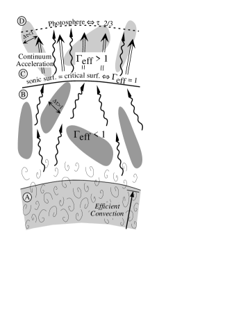
Figure 1: The proposed structure of a super-Eddington atmosphere (one with $L_{\mathrm{tot}}>{\cal L}_{\mathrm{Edd}}$) and the wind that it generates. The four regions, which are described in detail in the text, are: Region (A) A Convective envelope in which the radiation is sub-Eddington – $L_{\mathrm{rad}}<{\cal L}_{\mathrm{Edd}}<L_{\mathrm{tot}}$. Region (B) A porous atmosphere in which the effective Eddington luminosity is larger than the classical Eddington luminosity: ${\cal L}_{\mathrm{Edd}}<L_{\mathrm{rad}}=L_{\mathrm{tot}}<{\cal L}_{\mathrm{eff}}$. Region (C) of an optically thick, continuum driven wind, where perturbations are optically thin and the effective Eddington limit tends to the classical value. Region (D) of a photosphere and above.

The above considerations lead us to propose the following structure of a super-Eddington wind (hereafter SEW). Consider Fig. 1 for the proposed structure of a super-Eddington atmosphere (one with $L_{\mathrm{tot}}>{\cal L}_{\mathrm{Edd}}$) and the SEW that it generates. Four main regions can be identified in the atmosphere and they are:

• Region A: A Convective envelope – where the density is sufficiently high such that the excess flux above the Eddington luminosity is advected using convection. The radiative luminosity left is below the classical Eddington limit: $L_{\mathrm{rad}}<{\cal L}_{\mathrm{Edd}}<L_{\mathrm{tot}}$. It was shown by Joss, Salpeter & Ostriker ([Joss et al., 1973]) that convection is always excited before the Eddington limit is reached. Thus, if the density is high enough and the total flux is super-Eddington, this region has to exist.

• Region B: A zone with lower densities, in which convection becomes inefficient. Instabilities render the atmosphere inhomogeneous, thus facilitating the transfer of flux without exerting as much force. The effective Eddington luminosity is larger than the classical Eddington luminosity. ${\cal L}_{\mathrm{Edd}}<L_{\mathrm{rad}}=L_{\mathrm{tot}}<{\cal L}_{\mathrm{eff}}$. $\eta$ Car has shown us that the existence of this region allows for the steady state outflow during its 20 year long eruption ([Shaviv, 2000]).

• Region C: A region in which the effect of the inhomogeneities disappears and the luminosity is again super-Eddington. When perturbations arising from the instabilities, which are expected to be of order the scale height in size, become transparent, the effective opacity tends to the microscopic value and the effective Eddington limit tends to the classical value. At the transition between (B) and (C), the effective Eddington is equal to the total luminosity. This critical point is also the sonic point in a steady state wind. Above the transition surface, $L_{\mathrm{tot}}>{\cal L}_{\mathrm{eff}}\rightarrow{\cal L}_{\mathrm{Edd}}$ and we have a super sonic wind. This wind is expected to be optically thick.

• Region D: The photosphere and above. Since the wind is generally thick, the transition between regions (C) and (D) is far above the sonic surface.

2.3 The location of the critical point

Paramount to the calculation of the mass loss rate in super Eddington systems is the location of the critical point (separating regions (b) and (c) in Fig. 1), which corresponds to the sonic point of the wind generated at steady state. Therefore, we should try and estimate its location and density. Its definition is the location where the net average force on a gas element vanishes, or in other words, it is where the effective Eddington parameter $\Gamma_{\mathrm{eff}}$ is unity. To calculate it, we need to know the functional behavior of the effective opacity as a function of height.

The general behavior clearly depends on the characteristics of the nonlinear state of the porous atmosphere. However, this state is still part of an open problem under investigation and is therefore unknown. It will be shown, nevertheless, that the unknown geometrical factors that determine the mass loss can be pin-pointed while some other unknowns, such as $\Gamma_{\mathrm{eff}}$, actually cancel out to first approximation.

The effective opacity deep inside the atmosphere reduces $\Gamma$ to sub-Eddington values. However, higher up in the atmosphere where the perturbations become optically thin, the reduction in effective opacity diminishes to zero. In the thin limit, the effective opacity returns back to its microscopic value. We therefore write the opacity (per unit mass) of the medium as:

$${\kappa_{\mathrm{eff}}(\Delta\tau)\over\kappa_{0}}={\Gamma_{\mathrm{eff}}(\Delta\tau)\over\Gamma}={\Gamma_{\mathrm{eff},\infty}\over\Gamma}+(1-{\Gamma_{\mathrm{eff},\infty}\over\Gamma})\psi(\Delta\tau),$$ (2)

where $\Delta\tau$ is the equivalent optical width of a pressure scale height if the medium had been homogeneous. $\Gamma_{\mathrm{eff},\infty}$ is the effective $\Gamma$ in the limit of large optical depths. It is a function of $\Gamma$ which is unknown at this stage since we don’t have a model for the nonlinear behavior of the inhomogeneities. The function $\Gamma_{\mathrm{eff}}(\Delta\tau)$ should be obtained from a non linear model (which is part of work in progress). The function $\psi(\Delta\tau)$ gives the functional reduction of the opacity as a function of $\Delta\tau$. It should depend on the geometrical characteristics of the inhomogeneities. For $\Delta\tau\rightarrow 0$, $\psi\rightarrow 1$ and $\kappa_{\mathrm{eff}}$ will approach the microscopic value of the opacity $\kappa_{0}$. For large optical depths, we have $\Delta\tau\rightarrow\infty$, and obtain $\psi\rightarrow 0$ and $\kappa_{\mathrm{eff}}\rightarrow(\Gamma_{\mathrm{eff},\infty}/\Gamma)\kappa_{0}$.

Next, the sonic point for a steady-state transonic flow must be located at the critical point, where the local $\Gamma_{\mathrm{eff}}(\Delta\tau)$ is unity, i.e., where $(\kappa_{\mathrm{eff}}(\Delta\tau)/\kappa_{0})\Gamma=1$. We therefore have:

$$\psi(\Delta\tau_{\mathrm{sonic}})={1-\Gamma_{\mathrm{eff},\infty}\over\Gamma-\Gamma_{\mathrm{eff},\infty}}.$$ (3)

Let us assume that for small optical depths, $\psi(\Delta\tau\ll 1)\approx 1-{\cal A}\Delta\tau^{p_{l}}$ and that for large optical depths, $\psi(\Delta\tau\gg 1)\approx{\cal B}\Delta\tau^{-p_{h}}$. If we know the constants ${\cal A}$ and ${\cal B}$ and the powers $p_{l}$ and $p_{h}$, we can estimate the average density at the sonic point. To do that, we need a relation between the average density $\rho_{0}$ and $\Delta\tau$. To this goal we write the pressure scale height $l_{p}$ as

$$l_{p}={\nu v_{s}^{2}\over g(1-\Gamma_{\mathrm{eff},\infty})}.$$ (4)

The constant $\nu$ relates the effective speed of sound to the adiabatic one ($v_{s}$). If for example the atmosphere is isothermal, we have $\nu=1/\gamma$. If its temperature gradient is derived from radiation transfer and it has a constant opacity, we find $\nu=3/(4\gamma)$. The factor $1-\Gamma_{\mathrm{eff},\infty}$ originates from the ‘puffing-up’ of the atmosphere due to the radiative force (which reduces the effective gravity). Let the average density be $\rho_{0}$, then the optical width of a pressure scale height if the layer is homogeneous is given by:

$$\Delta\tau=\rho\kappa_{0}l_{p}={\rho\nu\kappa_{0}v_{s}^{2}\over g(1-\Gamma_{\mathrm{eff},\infty})},$$ (5)

therefore:

$$\rho=\rho_{{\mathrm{unit}}}\Delta\tau(1-\Gamma_{\mathrm{eff},\infty})\quad{\mathrm{with}}\quad\rho_{{\mathrm{unit}}}\equiv g/(\kappa_{0}\nu v_{s}^{2}).$$ (6)

For the small optical width limit, where $1-\psi\ll 1$, one has:

$$\rho_{\mathrm{sonic}}(\Delta\tau\ll 1) \approx \rho_{\mathrm{unit}}\Delta\tau_{\mathrm{sonic}}(1-\Gamma_{\mathrm{eff},\infty})$$

$$\approx \rho_{\mathrm{unit}}(1-\Gamma_{\mathrm{eff},\infty})\left({1\over{\cal A}}{\Gamma-1\over\Gamma-\Gamma_{\mathrm{eff},\infty}}\right)^{1\over p_{l}}.$$

However, small $\Delta\tau$’s are obtained when $1-\psi\ll 1$ or $\Gamma-1\ll\Gamma-\Gamma_{\mathrm{eff},\infty}$, namely, only when $\Gamma$ is very close to the Eddington limit. Under such conditions:

$$\rho_{\mathrm{sonic}}(\Delta\tau\ll 1)\approx\rho_{\mathrm{unit}}{1\over{\cal A}^{1\over p_{l}}}\left(\Gamma-1\right)^{1/p_{l}}(1-\Gamma_{\mathrm{eff},\infty})^{1-1/p_{l}}.$$ (8)

The opposite limit of large optical depths corresponds to $\psi\ll 1$, and consequently to $\Gamma\gg 1$ as well. In this limit we have:

$${1\over\Delta\tau_{\mathrm{sonic}(\Delta\tau\gg 1)}}\approx\left({1-\Gamma_{\mathrm{eff},\infty}\over\Gamma-\Gamma_{\mathrm{eff},\infty}}{1\over{\cal B}}\right)^{1/p_{h}}$$ (9)

or

$$\rho_{\mathrm{sonic}} \approx \rho_{\mathrm{unit}}(1-\Gamma_{\mathrm{eff},\infty})\Delta\tau_{\mathrm{sonic}}$$ (10)

$$\approx \rho_{\mathrm{unit}}{\cal B}^{1/p_{h}}\left(\Gamma-\Gamma_{\mathrm{eff},\infty}\right)^{1/p_{h}}\left(1-\Gamma_{\mathrm{eff},\infty}\right)^{1-1/p_{h}}$$

$$\approx \rho_{\mathrm{unit}}{\cal B}^{1/p_{h}}\left({\Gamma-1}\right)^{1/p_{h}}\left(1-\Gamma_{\mathrm{eff},\infty}\right)^{1-1/p_{h}}$$

where for the last approximation we used $\Gamma\gg 1\ga\Gamma_{\mathrm{eff},\infty}$.

Clearly, for the particular case of $p_{h}=p_{l}=1$ we obtain that both in the large and small optical depth regimes:

$$\rho_{\mathrm{sonic}}\approx\rho_{\mathrm{unit}}({\cal A}^{-1}~{}{\rm or}~{}{\cal B})(\Gamma-1).$$ (11)

It is interesting to note that for this particular set of power laws, both regimes do not depend on the value of $\Gamma_{\mathrm{eff},\infty}$ as it cancels out: The factor $1-\Gamma_{\mathrm{eff},\infty}$ introduced by the puffing up of the atmosphere cancels the factor $(1-\Gamma_{\mathrm{eff},\infty})^{-1}$ which appears because when the atmosphere is closer to the effective Eddington limit, smaller changes in the effective opacity are needed to reach the critical point.

We now proceed to show that the above simple power law scalings are indeed obtained under both limits. Since the arguments given are somewhat heuristic, the function $\psi(\Delta\tau)$ is also calculated analytically in the appendix for two simple cases under both limits, giving the same power laws. To strengthen the argumentation even more, we also use published results for an inhomogeneous system with a particular type of random statistical distribution (that of a Markovian statistics) for which the opacity (and $\psi$) can be calculated rigorously.

To find the power laws, we assume for simplicity that the medium is divided into regions of higher density $\rho_{h}\equiv{\bar{\rho}}(1+\delta)$ and volume $V_{h}\equiv\alpha V_{\mathrm{tot}}$ and regions of lower density $\rho_{l}\equiv{\bar{\rho}}(1-\delta)$ and volume $V_{l}\equiv(1-\alpha)V_{\mathrm{tot}}$. From conservation of mass it follows that $\rho_{h}V_{h}+\rho_{l}V_{l}=\rho_{0}V_{\mathrm{tot}}$ or ${\bar{\rho}}=\rho_{0}/(1+(2\alpha-1)\delta)$.

The optically thick limit: The optically thick limit can be generally described by Fig. 2. The reduced effective opacity is obtained by concentrating mass in dense ‘blobs’ and forming rarefied medium in between through which most of the radiation flux is funneled through. Simplistically, we have high density regions with a volume $V_{h}$, a density $\rho_{h}$ and a reduced flux $F_{h}$ and low density regions with $V_{l}$, $\rho_{l}$ and higher typical fluxes $F_{l}$.

In the absence of inhomogeneities, we would have had an average density $\rho_{0}$ and a flux $F_{0}$. For a given temperature gradient, we typically have $F_{h,l}\approx F_{0}\rho_{0}/\rho_{h,l}$. The result is accurate if the perturbations in the medium have a large vertical to horizontal aspect ratio, such that the temperature perturbations are negligible. Under more general perturbation geometries, this approximation is only a rough estimate but it should give the typical change expected in the fluxes.

The total average force $f$ acting on a volume which contains many inhomogeneous elements, is $f=\kappa_{0}(V_{h}\rho_{h}F_{h}+V_{l}\rho_{l}F_{l})\approx(V_{l}+V_{h})\kappa_{0}\rho_{0}F_{0}=f_{0}$, where $f_{0}$ is the force corresponding to the homogeneous case. That is, the average force does not change for a given fixed average temperature gradient. But the flux through the system is

$${F\over F_{0}} = {V_{h}F_{h}+V_{l}F_{l}\over F_{0}V_{\mathrm{tot}}}\approx\left({{V_{h}\over\rho_{h}}+{V_{l}\over\rho_{l}}}\right){\rho_{0}\over V_{\mathrm{tot}}}$$ (12)

$$= {1-\left[(2\alpha-1)\delta\right]^{2}\over 1-\delta^{2}}\equiv(\kappa_{0}/\kappa_{\mathrm{eff}})\geq 1.$$

We find an increased flux without changing the driving temperature gradient. Said in other words, the same temperature gradient drives now a higher flux—the radiative conductivity increases or the effective opacity decreases.

What happens though when the optical depth of the perturbations is finite? If we look at Fig. 2, we see that there exists a finite volume at the interface between the high density regions and the low density ones with a total cross section of about one optical depth. The material in this volume sees radiation from both the high density regions and the low density regions, so its flux will be averaged $F_{\mathrm{avr}}\approx(F_{h}+F_{l})/2$. The amount of mass that witnesses this averaged flux is of order the surface area $S$ of the interface between high and low density regions times ${\bar{\rho}}\kappa_{0}$. Half of the mass will be on the dense side (labeled ‘1’ in the figure) and occupy a volume of order $V_{1}\approx S/2\rho_{h}\kappa_{0}$ and the other half on the rarefied side (‘2’) and will occupy a larger volume $V_{2}\approx S/2\rho_{l}\kappa_{0}$. When calculated, the total force $f_{\mathrm{tot}}$ for a given temperature gradient remains unchanged, but the flux will not be as high:

$${F\over F_{0}}\hskip-3.0pt \approx \hskip-3.0pt{\rho_{0}\over V_{\mathrm{tot}}}\hskip-1.0pt\left[{V_{h}-V_{1}\over\rho_{h}}+{V_{l}-V_{2}\over\rho_{l}}+{V_{1}+V_{2}\over 2}\left({1\over\rho_{h}}+{1\over\rho_{l}}\right)\right]$$ (13)

$$\approx \hskip-3.0pt{F_{tot,\Delta\tau\rightarrow\infty}\over F_{0}}-{(V_{2}-V_{1})(\rho_{h}-\rho_{l})\rho_{0}\over 2V_{\mathrm{tot}}\rho_{h}\rho_{l}}$$

$$\approx \hskip-3.0pt{\kappa_{0}\over\kappa_{\mathrm{eff},\infty}}-{S\delta^{2}(1+(2\alpha-1)\delta)^{2}\over(1-\delta^{2})^{2}\kappa_{0}\rho_{0}V_{\mathrm{tot}}}$$

If we further assume that $\Gamma\gg 1$, then the significantly under-dense regions carry the lion share of the flux while the denser regions transport only a minor fraction. Under such conditions one can neglect $1/\rho_{h}$ when compared with $1/\rho_{l}$ or assume that $\delta$ is close to unity. We then obtain:

$${F\over F_{0}}\approx{\kappa_{0}\over\kappa_{\mathrm{eff},\infty}}-\left({\kappa_{0}\over\kappa_{\mathrm{eff},\infty}}\right)^{2}{S\over\kappa_{0}\rho_{0}4(1-\alpha)^{2}V_{\mathrm{tot}}}.$$ (14)

The effective opacity is then:

$${\kappa_{\mathrm{eff}}\over\kappa_{0}}={f\over f_{0}}{F_{avr}\over F_{\mathrm{tot}}}\approx{\kappa_{\mathrm{eff},\infty}\over\kappa_{0}}+{S\over 4(1-\alpha)^{2}\kappa_{0}\rho_{0}V_{\mathrm{tot}}}.$$ (15)

The more elaborate treatment in the appendix gives that the prefactor (again, for vertically elongated perturbations) is not $1/(4(\alpha-1)^{2})$ but $3/(32\alpha(\alpha-1)^{2})$ instead (i.e., 3/4 times smaller for $\alpha=1/2$).

The term $(S/2\kappa_{0}\rho_{0}V_{\mathrm{tot}})$ can be related to the optical depth of the perturbations. If the physical size of the perturbations is $d$, then we can write $S=\Xi V_{\mathrm{tot}}/d$, where $\Xi$ is an unknown geometrical factor. The geometrical factor is equal for example to 1 if the geometry is that of sheets of width $d$. It is higher for higher dimensionally of the structure (e.g., $\Xi\approx 2~{}{\rm or}~{}3$ for cylinders or spheres of diameter $d$, if $\alpha=1/2$).

If we now compare this result with the definition of the function $\psi$, we have:

$$1-\psi\approx{3S\over 32\alpha(1-\alpha)^{2}\kappa_{0}\rho_{0}V_{\mathrm{tot}}}\approx\left(3\Xi\over 32\alpha(1-\alpha)^{2}\right){1\over\beta}{1\over\Delta\tau},$$ (16)

where $\beta\equiv d/l_{p}$. It is the ratio between the typical size of the perturbations and the pressure scale height of the atmosphere. Since the typical wavelengths which are the quickest to grow are those with a size comparable to that of the scale height ([Shaviv, 2001]), this factor should too be of order unity but could be somewhat larger or smaller, depending on the details. The expression in parenthesis describes a geometrical factor which is of order unity or somewhat larger (e.g., if $\alpha=1/2$ then it is about 1-3 for typical $\Xi$’s, and it would typically be larger for other $\alpha$’s).

Through the definition of $\psi$ in the thick limit, we have

$${\cal B}={3\Xi\over 32\alpha\beta(1-\alpha)^{2}}\quad{\mathrm{and}}\quad p_{h}=1.$$ (17)

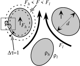
Figure 2: The effects of a finite optical depth on the flux and opacity of a system close to the thick limit. When the perturbations are optically thick, the fluxes inside and outside of the dense regions do not ‘mix’. However, because of the nonlocal nature of radiation transfer, a ‘blob’ with a finite optical width will have a region around its interface with the low density gas in which the radiative flux is averaged. Part of this interface region (denoted by ‘1’) has the high density, and part of it (denoted by ‘2’), has the lower density. The optical width of this region is of order unity. The result is that a finite fraction of the system’s volume is not effective in reducing the opacity.

The optically thin limit: We assume for simplicity that the medium is made up of spherical regions of higher density and those with lower density, each occupying a similar volume. Under this approximation, we can estimate both ${\cal A}$ and $p_{l}$ without cumbersome algebra.

The equation of radiative transfer for a gray atmosphere is:

$${dI({\bf x})\over ds}=\chi({\bf x})(B({\bf x})-I({\bf x})),$$ (18)

where $\chi=\kappa\rho$ and $B$ are the opacity per unit volume (i.e., the extinction) and radiation source function respectively.

The formal solution to the radiative equation for a point ${\bf x}$ located many optical distances from the boundary is (e.g., [Mihalas & Weibel Mihalas, 1984]):

$$I({\bf x},{\hat{\bf n}})=\int_{0}^{\infty}\chi({\bf x}-{\hat{\bf n}}s)B({\bf x}-{\hat{\bf n}}s)e^{-\int_{0}^{s}\chi({\bf x}-{\hat{\bf n}}s^{\prime})ds^{\prime}}ds.$$ (19)

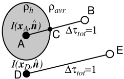
Figure 3: The effects of a finite optical depth on the flux and opacity of a system close to the thin limit. Point A located in a higher density region will witness a slightly reduced flux from the average one. The main reason is that when calculating the intensities $I({\bf x}_{A},\mu)$ at point A, the physical distance to a point B located an optical distance of unity from point A will be smaller than the distance D-E between two points with an average density between them, because the path A-C has a higher density. This short path will affect all photons coming from outside the dense region, giving a linear correction in $\rho_{0}\kappa_{0}d$. Because $I({\bf x}_{A},\mu)$ are sampled from a smaller volume, the first moment of $I$ which corresponds to the flux, will be smaller.

Next, we calculate the intensities $I({\bf x}_{A},{{\hat{\bf n}}})$ at point ‘A’ located inside a spherical region of radius $r_{0}$ with a density $\rho_{0}(1+\delta)$ (cf fig. 3). We assume that outside the given high density region the photons seen many high and low density regions and hence an average density. In other words, there is a high density correlation inside a given blob but it is assumed to be negligible for distances larger than the blob.

We also assume that the radiation source function is $B=B_{0}+bz$ and that there is no contribution from the perturbations. In the appendix, it will be shown to be a valid assumption because the correction to the source function is of second order, i.e., it falls as $(r_{0}\chi_{0})^{2}$. We also neglect higher order terms in $z$. We define now $\mu$ as the angle between the integration path and ${\hat{\bf z}}$. For simplicity, we also assume that $\alpha=1/2$.

Using the formal solution, the radiation intensity is then given by:

$$I({\bf x}_{A},{{\hat{\bf n}}})\hskip-3.0pt =\hskip-3.0pt B_{0}+\chi_{0}\cos(\mu)$$

$$\times\left[\int_{0}^{r_{0}}\chi_{0}s(1+\delta)\exp(-\chi_{0}s(1+\delta))ds\right.$$

$$\left.+\int_{r_{0}}^{\infty}s\exp(-\chi_{0}\rho_{0}((1+\delta)r_{0}+(s-r_{0}))\right]$$

$$\approx\hskip-3.0pt B_{0}+{b\over\chi_{0}}(1-\delta r_{0}\chi_{0})\cos\mu+{\cal O}(r_{0}\chi_{0})^{2}.$$ (21)

The flux is then given by:

$$F_{h}=F_{A}={1\over c}\oint I({\bf x}_{A},{{\hat{\bf n}}}){{\hat{\bf n}}}d\Omega=F_{0}(1-\delta)$$ (22)

where $F_{0}=4\pi b/(3c\chi_{0})$.

The flux in the under-dense regions is obtained by the transformation $\delta\rightarrow-\delta$. In the simplest case discussed here of both regions having the same volume fraction, we see that the total flux through the system remains unchanged. However, the mean force is now reduced:

$$f=V_{h}\rho_{h}\kappa_{0}F_{h}+V_{l}\rho_{l}\kappa_{0}F_{l}=f_{0}(1-r_{0}\kappa_{0}\rho_{0}\delta^{2}).$$ (23)

The effective opacity is therefore reduced as well. Using the result of eq. (12) for the thick limit and $\alpha=1/2$, and comparing to eq. (2) with $\psi(\Delta\tau\ll 1)\approx 1-{\cal A}\Delta\tau^{p_{l}}$, we finally get

$${\cal A}={\kappa_{0}\rho_{0}d\over 2\Delta\tau}={d\over 2l_{p}}=\beta/2\quad{\mathrm{a}nd}\quad p_{l}=1,$$ (24)

with $d=2r_{0}$. In other words, also in the thin limit, the function $\psi$ depends only on geometrical factors (and not for example on $\Gamma_{\mathrm{eff},\infty}$).

A Markovian mixture: A special case which can be solved more rigorously for any optical thickness is that of a Markovian mixture of dense and rarefied phases. A Markovian mixture is defined through the spatial statistics of the distribution: On any ray passing through the medium, the interface between material (or phase) A and material B form a Poisson process. In other words, if at point ${\bf s}$ the fluid is of type A, then at an infinitesimally close point ${\bf s}+d{\bf s}$, the probability of finding fluid B is $ds/\lambda_{0}$. If point ${\bf s}$ is in fluid B, then the equivalent probability of finding fluid A at point ${\bf s}+d{\bf s}$ is $ds/\lambda_{1}$. The effective transport properties in such a mixture were extensively analyzed by [Levermore et al. (1986)] and [Levermore et al. (1988)], and it is described in detail in §3.4 of [Pomraning (1992)]. It was found that the effective absorption cross-section in the absence of scattering is:

$$\sigma_{\mathrm{eff}}={(p_{0}\sigma_{0}+p_{1}\sigma_{1}+\sigma_{0}\sigma_{1}\lambda_{c})\over(1+(p_{0}\sigma_{1}+p_{1}\sigma_{0})\lambda_{c})},$$ (25)

with $\lambda_{c}\equiv{\lambda_{0}\lambda_{1}/(\lambda_{0}+\lambda_{1})}$, $p_{i}\equiv\lambda_{i}/(\lambda_{0}+\lambda_{1})$ and $\sigma_{0,1}$ being the two absoption cross-sections of materials $A$ and $B$ respectively. To translate this result to our problem notation, we identify $p_{0}$ with our $\alpha$, $p_{1}$ with $1-\alpha$ and $\lambda_{0}$ with $d$, such that $\lambda_{1}$ is $d(1-\alpha)/\alpha$ and $\lambda_{c}=(1-\alpha)d$. Moreover, we can identify $\sigma_{0}$ with $\rho_{h}\kappa_{0}$ and $\sigma_{1}$ with $\rho_{l}\kappa_{0}$. We then find that the effective opacity at the large optical depth limit is:

$${\kappa_{\mathrm{eff},\infty}\over\kappa_{0}}={1-\delta^{2}\over(1+(2\alpha-1)\delta)^{2}}.$$ (26)

Next, we write $d=\beta l_{p}$ and $\Delta\tau=l_{p}\rho_{0}\kappa_{0}$. Then, if we further assume that this reduction is large, as we did before, we can assume that $\rho_{h}\gg\rho_{l}$ or $\delta\approx 1$. Using this result, in the two optical depth limits ($\Delta\tau\ll 1$ for $\cal A$ and $\Delta\tau\gg 1$ for $\cal B$), it is straightforward to show that:

$${\cal A}=(1-\alpha)\beta\quad{\rm and}\quad{\cal B}={1\over(1-\alpha)\beta},$$ (27)

as well as $p_{h}=p_{l}=1$. Namely, in the special case of a Markovian mixture, we find that the function $\psi(\Delta\tau)$ behaves in the same way as in the simple models presented before, with only the normalization constants $\cal A$ and $\cal B$ being somewhat different but of the same order as before.

Although the analysis carried out here for the location of the critical point in both limits is far from accurate, it shows us that a simple formula (given by eq. 11) should describe the average density at the sonic point. Moreover, in both limits, the unknown constants depend only on geometrical factors such as the size of the perturbations in units of the pressure scale height ($\beta$) or the ratio $\Xi$ between the interface surface between high and low density regions and their volume in units of $d$, as well as on the particular shape the inhomogeneities adopt.

In both limits, the unknown constants ${\cal A}^{-1}$ and ${\cal B}$ were shown to be proportional to $\Delta\tau/\kappa_{0}\rho_{0}d=\beta^{-1}$. Since the perturbations are expected to be of the order of the scale height, this factor is of order unity as well. If the perturbations are smaller, the term will be larger and with it the density.

We define now a wind function ${\cal W}(\Gamma)$ such that:

$$\rho_{\mathrm{sonic}}\equiv\sqrt{\nu}{\cal W}(\Gamma)\rho_{\mathrm{unit}}(\Gamma-1)$$ (28)

(the factor $\sqrt{\nu}$ is introduced so that the ensuing wind mass-loss relation will not include it). From our analysis thus far, we found that if the geometrical properties of the developed inhomogeneities are not a function of $\Gamma$, then the prefactor to $(\Gamma-1)$ should be constant (but might be different for the two regimes: $\Gamma\gg 1$ and $\Gamma-1\ll 1$).

Since we have no information yet as to if and how the geometrical properties change with $\Gamma$, we assume in the remainder of the paper that they are constant and that the wind function is a constant as well. Thus,

$${\cal W}(\Gamma)={1\over\sqrt{\nu}}({\cal A}^{-1}~{}{\mathrm{or}}~{}{\cal B})\approx const.$$ (29)

We should emphasize that a simplifying assumption that we implicitly made is that the same proportionality relation exists for the large and the small optical depths. This is found to be the case in the Markovian mixture of low and high density regions. However, this need not be the general case.

We should also bare in mind that the transition between the two normalizations (i.e., a different ${\cal W}$ for the optically thick and thin cases) should take place at $\Gamma-1\sim 1-\Gamma_{\mathrm{eff},\infty}\la 1-\Gamma_{\mathrm{crit}}\approx 0.15-0.5$ (depending on the type of instability that governs). This will actually be below the typical $\Gamma$’s we will obtain in the analysis. That is, we are mainly concerned with the optically thick limit. We should also be cautious because the function $\psi(\Delta\tau)$ could in principle also be a function of $\Gamma$ (and therefore the constants ${\cal A}$ and ${\cal B}$ as well), especially if the geometrical behavior of the inhomogeneities changes with $\Gamma$. For example, if the typical optical depth of the ‘blobs’ is $\Gamma$ dependent. Only a detailed numerical analysis could shed more light on this problem.

The next step in the analysis presented here is to follow the nonlinear characteristics of the inhomogeneities. This is an intrinsically difficult problem since it requires the radiation-hydrodynamical understanding of the saturation properties of the instabilities in the medium. This analysis has commenced in the form of a detailed hydrodynamic simulation. A different approach which will soon be completed, is to find empirically ${\cal W}$ and any possible $\Gamma$ dependence. This can be performed by solving for the super-Eddington counterpart to the core-mass luminosity relation ([Paczynski, 1970]) which should describe the steady state of novae in their post-maximum decline. Then, by comparing to novae, both $\Gamma_{\mathrm{eff},\infty}$ and ${\cal W}$ can be extracted for novae with different luminosities.

2.4 The mass loss rate

Once we have estimated the density at the sonic point, we can proceed to calculate the mass loss rate. It is given by: $\dot{M}=4\pi R_{0}^{2}\rho_{\mathrm{sonic}}v_{\mathrm{sonic}}$, where the relevant speed of sound is $v_{\mathrm{sonic}}=\sqrt{\nu}v_{s}$. This speed is generally not the adiabatic speed of sound since the flow isn’t adiabatic.

Using eq. (28), we find:

$$\dot{M} = 4\pi R_{0}^{2}\rho_{{\mathrm{sonic}}}v_{{\mathrm{sonic}}}={4\pi GM_{\star}{\cal W}(\Gamma)(\Gamma-1)\over\kappa_{0}v_{s}}$$ (30)

$$= {{\cal W}(\Gamma)(L-{\cal L}_{\mathrm{Edd}})\over cv_{s}}.$$

Note that ${\cal L}_{\mathrm{Edd}}$ becomes the modified Eddington luminosity if the underlying opacity is not that of Thomson scattering. Eq. (30) is the basic result of the present theory.

From the analysis of the location of the critical point in §2.3, we have seen that ${\cal W}$ should be of order unity or somewhat larger if the size of the perturbations $d$ is similar to the pressure scale height of the atmosphere (since $\cal W$ scales with $l_{p}/d$). Moreover, since $\cal W$ depends only on the geometrical properties of the perturbations, it could be close to a constant if these properties are not a function of $\Gamma$. Hence, we assume for simplicity that ${\cal W}(\Gamma)$ is a constant of order unity. We iterate once more that it is only with a more elaborate simulation or with more accurate and careful observations, that a more accurate functional form can be deduced. For the meantime, we will have to settle with this simplifying yet reasonable assumption.

We will show in the rest of the paper that eq. (30) provides an explanation to the mass loss from bright classical novae as well as from $\eta$ Carinae and allows us to connect between the observed luminosity and mass loss rate, a relation which hitherto did not exist for super-Eddington systems.

2.5 High Load winds

Unlike normal stellar winds, the thick winds formed in the super-Eddington flows not only have a high mass momentum relative to the total radiative momentum, which is expected in any thick wind, but more importantly, the kinetic energy flux can be comparable to the radiative luminosity. It also inadvertently implies that the rate of gravitational energy ‘pumped’ into the outflowing matter is also comparable. Consequently, the luminosity $L$ in eq. (30) is not the observed luminosity at infinity. Instead, we have to substitute $L_{0}$ for $L$ where

$$L_{0}\approx L_{\mathrm{tot}} = L_{\infty}+\dot{M}\left({v_{\infty}^{2}\over 2}+{GM_{\star}\over r_{0}}\right)$$ (31)

$$= L_{\infty}+{\dot{M}\over 2}(v_{\infty}^{2}+v_{\mathrm{esc}}^{2}).$$

(The approximation neglects the kinetic energy at the sonic points, i.e., assuming that $v_{s}^{2}\ll v_{\mathrm{esc}}^{2}$ which gives $L_{\mathrm{tot}}\approx L_{0}$). The effect of a lowered observed luminosity was coined ‘photon tiring’ by Owocki & Gayley ([Owocki & Gayley, 1997]), who solved for the behaviour and evolution of the wind. Their solution related the variables $L_{\infty},L_{0},\dot{M},v_{\infty}^{2}$ and $v_{\mathrm{esc}}^{2}$. The basic equations are the equations of continuity, momentum conservation and energy conservations:

$$\dot{M} = const=4\pi r^{2}v\rho$$ (32)

$${1\over 2}{dv^{2}\over dr} = -{GM_{\star}(1-\Gamma(r))\over r^{2}}$$ (33)

$$L(r) = L_{0}-\dot{M}\left[{v^{2}\over 2}+{GM_{\star}\over R_{0}}-{GM_{\star}\over r}\right],$$ (34)

where $\Gamma(r)$ is the ratio between the luminosity $L(r)$ and the local modified Eddington luminosity ${\cal L}_{\mathrm{Edd}}$ which we assumed to be constant, since the opacity is assumed to be given by the Thomson scattering. The solution to this set of equations, after neglecting the speed of sound at the base of the wind, is ([Owocki & Gayley, 1997]):

$$w\equiv{v^{2}\over v_{\mathrm{esc}}^{2}}=-x+{\Gamma_{0}\over{\tilde{m}}}\left(1-\exp(-{\tilde{m}}x)\right),$$ (35)

where $x$ is defined as $1-{R_{0}/r}$. $R_{0}$ is the radius of the sonic point of the wind and can be described as the ‘hydrostatic’ radius of the star. Below it, the envelope is expanding with a subsonic speed. ${\tilde{m}}$ is defined as $\dot{M}GM_{\star}/{\cal L}_{\mathrm{Edd}}R_{0}$. It is a slightly different definition for the ‘photon tiring number’ than the original definition of $m$ by Owocki & Gayley ([Owocki & Gayley, 1997]). The two are related through ${\tilde{m}}=\Gamma_{0}m$.

At very large radii ($r\rightarrow\infty$), we have

$$w_{\infty}={v_{\infty}^{2}\over v_{\mathrm{esc}}^{2}}=-1+{\Gamma_{0}\over{\tilde{m}}}\left(1-\exp(-{\tilde{m}})\right).$$ (36)

Using the wind model developed here (eq. 30), we can close the relation between $\dot{M}$ (or ${\tilde{m}}$) and the luminosity ($\Gamma_{0}{\cal L}_{\mathrm{Edd}}$) of the star:

$${\tilde{m}}={1\over 2}{v_{\mathrm{esc}}^{2}\dot{M}\over{\cal L}_{\mathrm{Edd}}}={1\over 2}{v_{\mathrm{esc}}^{2}{\cal W}\over v_{s}c}(\Gamma_{0}-1)\equiv(\Gamma_{0}-1){\tilde{W}},$$ (37)

where ${\tilde{W}}$ is the ‘scaled’ wind parameter. This is a dimensionless version of eq. (30) – the basic mass-loss luminosity relation of SEWs.

For given $\Gamma_{0}$, ${\cal L}_{\mathrm{Edd}}$ and $R_{0}$ (or $v_{\mathrm{esc}}^{2}$), we can now calculate ${\tilde{m}}$ (or $\dot{M}$), and from it calculate $w_{\infty}$ (or $v_{\infty}^{2}$) and $\Gamma_{\infty}$. To get the latter, we substitute the energy conservation equation into the equation for $w$ to get:

$$\Gamma_{\infty}=\Gamma_{0}\exp(-{\tilde{m}}).$$ (38)

In order to compare with observations, we need to translate $L_{\infty}$, $\dot{M}$ and $v_{\infty}$, into an observed temperature. This is done using a steady state optically thick wind model. When integrated upwards, a photosphere should be obtained where the optical depth is of the order of 2/3. The general case is far from trivial because the opacity is $\sim\sqrt{\kappa_{\mathrm{sc}}\kappa_{\mathrm{ab}}}$ where $\kappa_{\mathrm{ab}}$ is the absorptive opacity which is generally much smaller than the scattering opacity. The simplest approximation is first to assume that the opacity is that of Thomson scattering. This was done when the original steady state optically thick wind explanation to novae was proposed ([Bath & Shaviv, 1976]). It yields an effective temperature that satisfies the following equation:

$$\log\left(\dot{M}\over\mathrm{gr~{}s^{-1}}\right) = 22.0-2.0\log\left(T_{\mathrm{eff}}\over 10^{4}~{}\mathrm{{}^{\circ}K}\right)$$

$$\hskip-34.14322pt+\log\left(v\over 10^{8}\mathrm{~{}cm~{}s^{-1}}\right)+0.5\log\left(L_{\infty}\over 10^{38}\mathrm{~{}erg~{}s^{-1}}\right).$$

In reality though, the absorption opacity is lower and the photosphere is deeper in the wind, where the temperature is higher. Thus, a temperature estimate based on eq. (2.5) will be adequate only when we use an effective temperature that is defined through $\sigma T_{\mathrm{eff}}^{4}\equiv L/4\pi r_{\mathrm{ph}}^{2}$, where $r_{\mathrm{ph}}$ is the radius where the optical depth for the continuum becomes $2/3$. This temperature is used, for example, in the analysis by Schwarz et al. ([Schwarz et al., 1998]). If a real colour temperature is needed (such as by comparison to a Planckian spectrum), then a more extended analysis, as was carried out by Bath ([Bath, 1978]) is needed. Since we do not require a very accurate mass loss temperature relation (as the measurement error in the observations is much larger anyway), a simple fit to Bath’s results is sufficient. One obtains that for $T_{\mathrm{colour}}\ga 6000^{\circ}{\mathrm{K}}$, the relation is:

$$\log\left(\dot{M}\over\mathrm{gr~{}s^{-1}}\right) = 22.3-1.48\log\left(T_{\mathrm{colour}}\over 10^{4}\mathrm{{}^{\circ}K}\right)$$

$$\hskip-39.83368pt+\log\left(v\over 10^{8}\mathrm{~{}cm~{}s^{-1}}\right)+0.65\log\left(L_{\infty}\over 10^{38}\mathrm{~{}erg~{}s^{-1}}\right).$$

It provides an estimate to $\log\dot{M}$ that is better than $0.1$, which is more than sufficient for our purpose here.

Both eqs. (2.5) & (2.5) can be written more generally as

$${\dot{M}\over\dot{\bar{M}}}={(v_{\infty}/\bar{v}_{\infty})(L_{\infty}/\bar{L})^{p_{L}}\over(T_{i}/\bar{T})^{p_{T}}},$$ (41)

where $T_{i}$ is either $T_{\mathrm{eff}}$ or $T_{\mathrm{colour}}$ and $\dot{\bar{M}},\bar{v}_{\infty},\bar{L},\bar{T},p_{L}$ and $p_{T}$ are constants read off eqs. (2.5) & (2.5). This expression allows us to treat both cases simultaneously.

The last relation that we need in order to close the set of equations is the exact value of $v_{s}$ at the base of the wind. To this goal we need the temperature at the base of the wind. For simplicity, we assume that the velocity is constant and equal to the terminal value; in other words, most of the acceleration takes place deep in the optically thick part. This assumption is valid as long as $r_{\mathrm{ph}}\gg R_{0}$. Under these conditions, the temperature at the bottom can be estimated to be:

$$T_{0}\approx T_{\mathrm{i}}\left(r_{\mathrm{ph}}\over R_{0}\right)^{3/4}\left(\Gamma_{0}\over\Gamma_{\infty}\right)^{1/4}.$$ (42)

When we work with the colour temperature, $r_{\mathrm{ph}}$ is the depth of the last mean emission (i.e., $\tau=2/3$ for an opacity of $\sqrt{\kappa_{\mathrm{sc}}\kappa_{\mathrm{ab}}}$).

On one hand, the mass loss depends on the parameters of the sonic point (e.g., $R_{0}$ or $v_{\mathrm{esc}}$, and $T_{0}$). On the other hand however, these parameters depend on the photospheric conditions (e.g., through eq. 42). Therefore, the parameters of the wind, the conditions at the sonic point and the conditions at the photosphere should all be solved self consistently. It is carried out as follows:

Assume that the mass of an object $M_{\star}$, its Eddington parameter at the base $\Gamma_{0}$, and a scaled wind parameter ${\tilde{W}}$ are given. To obtain the complete wind, sonic point and photospheric parameters we begin by calculating ${\tilde{m}}$ using eq. (37). Next, $\Gamma_{\infty}$ (and $L_{\infty}$) are found using eq. (38). $w_{\infty}$ is then obtained using eq. (36). To obtain the remaining parameters, we have to combine together the rest of the equations. These are eqs. (37), (42), and (41). The latter corresponds to either eq. (2.5) or eq. (2.5), depending on whether we work with the effective temperature $T_{\mathrm{eff}}$ or the colour temperature $T_{\mathrm{colour}}$. To close the relations we need three more equations, which are $v_{\mathrm{esc}}^{2}=2GM_{\star}/R_{0}$, $v_{s}=\sqrt{\gamma kT_{0}/\mu m_{H}}\equiv\bar{v}_{s}\sqrt{T_{0}/\bar{T}}$ and $\sigma T_{i}^{4}=L_{\infty}/4\pi r_{ph}^{2}$ . When combined, we find the following expressions for $T_{i}$, $v_{\infty}$ and the mass loss $\dot{M}$:

$$T_{i} \hskip-7.0pt=\hskip-7.0pt \hskip-3.0pt\left[c^{12}{\cal L}_{\mathrm{Edd}}^{5p_{L}-{11\over 4}}\dot{\bar{M}}^{5}\bar{T}^{5p_{T}-6}\bar{v}_{s}^{12}w^{5\over 2}{\tilde{W}}^{12}\Gamma_{0}^{3\over 2}\Gamma_{\infty}^{{3\over 4}+5p_{L}}\over 4\pi^{9\over 4}\sigma^{9\over 4}G^{9\over 2}\bar{L}^{5p_{L}}{\tilde{m}}^{5}M_{\star}^{9/2}\bar{v}_{\infty}^{5}{\cal W}^{12}\right]^{1\over 3+5p_{T}}$$

$$v_{\infty} \hskip-7.0pt=\hskip-7.0pt \hskip-3.0pt\left[{2\bar{L}^{p_{L}}{\tilde{m}}\bar{v}_{\infty}w\over\Gamma_{\infty}^{p_{L}}{\cal L}_{\mathrm{Edd}}^{p_{L}-1}\dot{\bar{M}}}\left(2c^{4}\bar{v}_{s}^{4}{\tilde{W}}^{4}\Gamma_{0}^{1\over 2}\Gamma_{\infty}^{1\over 4}{\cal L}_{\mathrm{Edd}}^{3\over 4}w^{5\over 2}\over\pi^{3\over 4}\sigma^{3\over 4}G^{3\over 2}M_{\star}^{3\over 2}\bar{T}^{3}{\cal W}^{4}\right)^{p_{T}}\right]^{1\over 3+5p_{T}}$$

$$\dot{M} \hskip-7.0pt=\hskip-7.0pt \hskip-3.0pt\left[{2{\cal L}_{\mathrm{Edd}}^{1+2p_{L}}{\tilde{m}}\dot{\bar{M}}^{2}w\Gamma_{\infty}^{2p_{L}}\over\bar{L}^{2p_{L}}}\right.$$ (43)

$$\left.\times\left(8\pi^{3\over 8}G^{3}{\cal L}_{\mathrm{Edd}}^{7\over 2}{\tilde{m}}^{5}M_{\star}^{3}\bar{T}^{6}{\cal W}^{8}\sigma^{3\over 2}\over c^{8}\bar{v}_{s}^{8}{\tilde{W}}^{8}\Gamma_{0}\Gamma_{\infty}^{1\over 2}\right)^{p_{T}}\right]^{1\over 3+5p_{T}}.$$

The expressions for the additional parameters can be found in a straightforward manner.

The contour plots of $\Gamma_{\infty}(\Gamma_{0},{\tilde{W}})$, $v_{\infty}(\Gamma_{0},{\tilde{W}})$ and $T_{\mathrm{colour}}(\Gamma_{0},{\tilde{W}})$ are depicted in Fig. 4 for a $1M_{\sun}$ system.

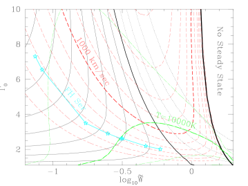
Figure 4: The state solution in the $\Gamma_{0}$ - ${\tilde{W}}$ plane. Here, $\Gamma_{0}$ is the Eddington parameter at the base of the wind, while ${\tilde{W}}$ is the scaled wind parameter describing the relative ‘load’ of the wind ${\tilde{W}}\equiv Wv_{\mathrm{esc}}^{2}/2v_{s}c$. Larger ${\tilde{W}}$’s imply a smaller base radius. The thin continuous set of lines is lines of constant $\Gamma_{\infty}>1$. The separation between two consecutive lines is 0.2 dex. The set of dotted lines is lines of constant $\Gamma_{\infty}<1$ separated by 0.2. The $\Gamma_{\infty}=1$ line separating between the two sets of lines, is marked heavier. The dashed set of lines is lines of constant $v_{\infty}$ separated by $100$ km s^-1. The asymptotic line of $v_{\infty}=0$, beyond which there is no steady state wind solution, is marked as a thick line. The dot-dash set of lines describe constant colour temperatures separated by 2500K. Note that the lower lines are the hotter ones. The evolution of FH Ser is marked by stars connected with a continuous line. The evolution of FH Ser from top left to bottom right was calculated by combining the following equations as explained in the text: (a) The wind model to relate $\dot{M}$ to $\Gamma_{0}$ (given in this work), (b) The temperature mass loss relation (given by Bath 1978), and (c) Relations between the observed parameters and the parameters at the base of the wind (given by Owocki & Gayley 1997). The stars are the values obtained at different days from the data of Friedjung (1987). The fact that the light curve conspicuously follows an iso-$v_{\infty}$ contour arises because the observed $v_{\infty}$ for FH Serpentis happens to vary only little, from 670 to 770 km s^-1.

3 Application of the SEW theory

We now proceed to apply the SEW theory to systems that clearly exhibited super-Eddington outflows over long durations relative to the dynamical time scales.

3.1 Two super-Eddington nova

Although many novae display super-Eddington luminosities for at least short periods, it is often difficult to unequivocally show that a particular nova was indeed super-Eddington for a long duration, even if it was. The reason is that during the ‘bolometric plateau’ that a nova exhibits, the luminosity can be close to the Eddington limit (from either above or below it) such that even small uncertainties in distance and luminosity can hide the true nature of the flow. Moreover, since the wavelength of maximum emission shifts to the UV during the ‘bolometric plateau’, as the temperature increases, it is difficult to acquire accurate bolometric luminosities from Earth based observations. Our insistence of using good data results with having only two clear cases in which long duration super-Eddington flows were observed and have good enough data. The two cases are Nova LMC 1988 #1 and Nova FH Serpentis. Other cases such as V1500 Cygni are not as clear cut, even though one would suspect that long duration SEWs could have been present. In V1500 Cygni, the nova was observed to shine at significantly super-Eddington luminosities for a few days after the eruption, and when observed again on day 100, it was 2/3 of Eddington. Thus, there is no clear indication for the duration of the super-Eddington episode, only a lower limit. Another recent example is Nova LMC 1991, which was observed to be super-Eddington for two weeks ([Schwarz et al., 2000]), reaching a truly impressive luminosity as high as $2.6\pm 0.3\times 10^{39}$ erg s^-1! As we shall soon see, both V1500 Cygni and LMC 1991 were classified as very fast novae and hence are marginally useful candidates for a steady state analysis. Another nova, V1974 Cygni 1992, had very beautiful bolometric observations ([Shore et al., 1994]) which could have been potentially very useful for the analysis done here. Unfortunately, the distance uncertainty of 1.8 to 3.2 kpc ([Paresce et al., 1995]) corresponds to more than a factor of 3 uncertainly in the bolometric luminosity, which is too large.

3.1.1 Nova LMC 1988 #1

Nova LMC 1988 #1 occurred, as the name suggests, in the LMC. Thus, its distance is known more accurately than the distance of galactic novae. This distance, coupled to an extensive multi-wavelength campaign by Schwarz et al. ([Schwarz et al., 1998]), resulted with their rather accurate finding that Nova LMC 1988 #1 had an average bolometric luminosity of $(3.0\pm 0.3)\times 10^{38}\mathrm{~{}erg~{}s^{-1}}$ during the first 45 days after visual maximum. By considering that the maximum mass a WD can have is $1.4~{}M_{{\sun}}$, Schwarz et al. ([Schwarz et al., 1998]) concluded that the nova had to be super-Eddington for the long duration. We use their data and results for the analysis. This includes the evolution of the bolometric luminosity and the effective temperature (as opposed to a colour temperature).

3.1.2 Nova FH Serpentis

Nova FH Serpentis is less clear than Nova LMC 1988 #1. Specifically, an accurate distance determination was obtained only after using the HST measurement of the expanding ejecta ([Gill & O’Brien, 2000]). The reddening which is inaccurately known (and is probably in the range $E(B-V)=0.64\pm 0.16$, [della Valle et al., 1997]) then remains as the main source of error in the bolometric luminosity determination. If we take the determination of the possible range for the bolometric luminosity by Duerbeck ([Duerbeck, 1992]) and della Valle et al. ([della Valle et al., 1997]) and correct for the somewhat larger distance determined by Gill & O’Brien ([Gill & O’Brien, 2000]), we find that the bolometric luminosity on day 6.4, when the first UV measurement was taken, is $M_{\mathrm{bol}}=-7\aas@@fstack{m}5\pm 0\aas@@fstack{m}2$, namely, $L$ must have been more than $2.5\times 10^{38}\mathrm{~{}erg~{}s^{-1}}$.

Furthermore, since the total mass ejected has a lower bound of $5\times 10^{-5}~{}M_{{\sun}}$, and is probably more of the order of $2\times 10^{-4}~{}M_{{\sun}}$, we should take the kinetic energy of the outflow into account. Since the ejecta is moving at about $500~{}\mathrm{km~{}s^{-1}}$ ([Gill & O’Brien, 2000]), the ejecta has a minimum kinetic energy of $2.5\times 10^{44}~{}\mathrm{erg}$. A lower estimate to the contribution of the kinetic energy to the total flux at the base of the wind would be to divide the kinetic energy uniformly over the duration of the bolometric plateau that lasted about 45 days. This gives a minimum contribution of $L_{\mathrm{kin,min}}=6.5\times 10^{37}~{}\mathrm{erg~{}s^{-1}}$. Since the total mass loss is probably higher than $5\times 10^{-5}~{}M_{{\sun}}$ and since the mass loss rate was likely to be higher than average when the luminosity was higher than the average luminosity, it is likely that $L_{\mathrm{kin}}>L_{\mathrm{kin,min}}$ on day 6.4. When we add the kinetic energy to the observed bolometric luminosity at day 6.4, we find that $L_{\mathrm{tot}}$ at the base of the wind must have been at least $3.1\times 10^{38}\mathrm{~{}erg~{}s^{-1}}$. Clearly, even if the mass of the WD is large (which is inconsistent with the eruption not being a very fast nova), the luminosities are super-Eddington. The fact that the kinetic energy necessarily implies that the nova was super-Eddington (at the base of the wind) was already pointed out by Friedjung ([Friedjung, 1987]) who did not have observations on the mass ejected but instead used photospheric constraints on $\dot{M}$. Here, we have reached the same conclusion without resorting to the photospheric analysis. This could be done due to the better distance measurements (which are within the error but on the high side of previous estimates), and better reddening measurements of della Valle et al. ([della Valle et al., 1997]).

We use the data of Friedjung ([Friedjung, 1987], also in [Friedjung, 1989]) for the behaviour of the temperature, luminosity and velocity at infinity. These data are based on the UV measurements by Gallagher & Code ([Gallagher & Code, 1974]) and in addition include the integrated flux that falls outside the UV range observed by Gallagher & Code assuming a black body distribution. We correct the luminosities to include the better distance determination by Gill & O’brian ([Gill & O’Brien, 2000]).

3.2 Is a steady state model appropriate for the ‘bolometric plateau’ of novae?

A steady state model is probably appropriate for two reasons:

1. Circumstantial evidence: Kato & Hachisu ([Kato & Hachisu, 1994]) compared their steady state model for winds to the results of a dynamical evolution of Prialnik ([Prialnik, 1986]) and found relatively good agreement, implying that a steady state solution is valid for most of the nova evolution.

2. Physical reasons: A wind with a terminal velocity of $v_{\infty}$ originates from a typical radius $r_{0}$ that has an escape velocity of order $v_{\infty}$. Two conditions should therefore be satisfied for the wind to be in a steady state. First, the sub-sonic region beneath the base of the wind should be acoustically connected on time scales shorter than the typical evolution time of the system. Namely:

   $$t_{\mathrm{sub-sonic}}\approx{r_{0}\over v_{s}}\ll t_{\mathrm{evolution}}.$$ (44)

   The second criterion is that the time it takes the accelerated material to reach the photosphere is shorter than the time at question:

   $$t_{\mathrm{super-sonic}}\approx{r_{\mathrm{ph}}\over v_{\infty}}\ll t_{\mathrm{evolution}},$$ (45)

   where $t_{\mathrm{evolution}}$ is the typical time scale for changes in the system. Both Nova FH Serpentis and Nova LMC 1988 #1 satisfy both requirements from days 4 and 2 onward respectively. Thus, a steady state solution for the objects ought to be found for $t_{\mathrm{evolution}}\approx{\mathrm{m}onth}$. As previously mentioned, Novae V1500 Cygni and LMC 1991 do not satisfy the required conditions – they are very fast novae that evolve dramatically on a time scale of days, so a steady state wind cannot be assumed in their analysis.

3.3 Application to Nova FH Serpentis

Using the described method of analysis, we proceed to fit the data of Friedjung ([Friedjung, 1987]) which includes $T_{\mathrm{colour}}$, $L_{\infty}$ and $v_{\infty}$. Given a wind parameter ${\cal W}$, a white dwarf mass $M_{\mathrm{WD}}$ and a hydrogen mass fraction $X$, we solve for, at each observed point, the values of $\Gamma_{0}$ and ${\tilde{W}}$ which result with the observed $v_{\infty}$ and $\Gamma_{\infty}$. This is done iteratively. That is, $\Gamma_{0}$ and ${\tilde{W}}$ are assumed to be known such that $\Gamma_{\infty}$ and $v_{\infty}$ can be calculated according to the procedure described at the end of §2.5. Then, $\Gamma_{0}$ and ${\tilde{W}}$ are varied until the calculated $\Gamma_{\infty}$ and $v_{\infty}$ agree with observations. (A function of $\Gamma_{0}$ and ${\tilde{W}}$ is defined such that its value is the error between the observations and the obtained values of $\Gamma_{\infty}$ and $v_{\infty}$. The function is then minimized using a maximum ‘downhill’ gradient method).

The resulting set of $\Gamma_{0}$ and ${\tilde{W}}$ for each observation point is then used to predict a colour temperature. The predicted temperatures are then compared with the observed temperatures (and their error) to give a $\chi^{2}$ number.

The results for $X=0.3,0.7$ are depicted in Fig. 5. We find that the possible $1-\sigma$ range for ${\cal W}$ is about 21.5 to 34. If we allow larger statistical variation of $3-\sigma$ then the value of ${\cal W}$ can range from 20 to about 39.5 (if we restrict ourselves to a reasonable WD mass range between 0.6 and 1.0 solar masses, as the decay rate $t_{3}$ would suggest it is).

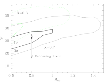
Figure 5: The $\chi^{2}$ fit of the predicted temperature (from the luminosity and wind theory) to the observed temperature variations of Nova FH Serpentis, for two values of the Hydrogen mass fraction $X$. The 1 and 3 $\sigma$ statistical variation contours are marked in the ${\cal W}$ – $M_{\mathrm{\mathrm{WD}}}$ plane. Good fits are obtained for reasonable parameters. A $\chi^{2}$ of 4.2 is obtained for $8-2=6$ degrees of freedom. The systematic errors are large and arise from the inaccurate knowledge of $M_{\mathrm{\mathrm{WD}}}$, $X$ and the reddening to Nova FH Serpentis. The limit on the systematic variation of the latter is given by the arrows.

An additional systematic error arises from the inaccuracy of the derived reddening of Nova FH Serpentis. This uncertainty is portrayed by the error which could increase or decrease the derived ${\cal W}$ by roughly +1.8 or -7.2 respectively.

Fig. 6 depicts the observed colour temperature evolution and the predicted colour temperature evolution using the best fit values of ${\cal W}$, $\Gamma_{\infty}(t)$ and ${\tilde{W}}(t)$, and the nominal values of $X=0.7$ and $M_{\mathrm{\mathrm{WD}}}=0.8M_{{\sun}}$. Good agreement between the predicted temperature using the SEW theory and the observed colour temperature can be obtained, clearly demonstrating that the theory is consistent.

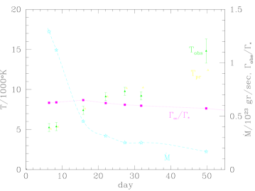
Figure 6: The observed colour temperature behaviour $T_{\mathrm{obs}}$ of Nova FH Serpentis (filled triangles, taken from Friedjung 1987) as compared with the predicted colour temperature behaviour $T_{\mathrm{pr}}$ from the observed luminosity and wind model (open triangles, slightly offsetted to the right), for the best fit model assuming $M_{\mathrm{\mathrm{WD}}}=0.8M_{\sun}$ and $X=0.70$. The additional plots are of the mass loss (the stars and dashed line). The mass loss integrates to $8\times 10^{-5}M_{{\sun}}$. Finally we plot as filled squares the ratio of $\Gamma_{\infty}$ to $\Gamma_{0}$. Apparently, about 40% of the original radiative luminosity at the base of the wind is used-up under these parameters to accelerate the wind and compensate for its potential energy. Clumpiness will reduce this fraction.

The temporal evolution of the observed luminosity, as given in the same figure, can be integrated to obtain a total mass loss of $8\times 10^{-5}M_{{\sun}}$. The main source of uncertainty in this figure is again the reddening which could increase or decrease the mass loss by about +10% and -30% respectively. This result is completely consistent with the observational range of $(2-20)\times 10^{-5}M_{{\sun}}$ ([Hack et al., 1993], [Gill & O’Brien, 2000]).

An important point which should be considered is that the wind is likely to be clumpy, a fact which the analysis thus far did not take into account. In the region around the sonic point, the optical depth of typical clumps is expected to be of order unity. Above this point, typical clumps are therefore expected to be optically thin. Thus, the main effect of the clumpiness is to increase the effective absorptive opacity (since one will then obtain that $\kappa_{\mathrm{a}b}\propto\sqrt{\left<\rho^{2}\right>}>\sqrt{\left<\rho\right>^{2}}$). The effective opacity which is proportional to the geometric mean of the scattering and absorptive opacities will increase as $\sqrt{{\cal C}}$ where ${\cal C}$ is a clumpiness parameter:

$${\cal C}\equiv\sqrt{\left<\rho^{2}\right>/\left<\rho\right>^{2}}.$$ (46)

Moreover, from Bath & Shaviv ([Bath & Shaviv, 1976]) we have that for a fixed temperature, outflow velocity and luminosity, the inferred mass loss rate is proportional to $\kappa^{-3/2}$. Thus, a first guess would be that by assuming homogeneity we over estimate ${\cal W}$ by roughly a factor of ${\cal C}^{3/4}$. A more detailed analysis which repeats the fitting actually shows that the power law relation is over estimated by about 10-15%. That is to say, ${\cal W}$ is over estimated by about ${\cal C}^{0.67}$ for $M_{\mathrm{W}D}\sim(0.8-1.0)M_{\sun}$.

We do not know what the value of ${\cal C}$ should be. A rough guesstimate would be to take the value found in another type of system in which strong optically thick winds are observed, namely, WR stars. In binary systems in which one of the stars is a WR, several measurements of the mass loss in the winds can be performed. Some (which are usually the more difficult ones) measure the actual mass loss $\dot{M}$ (for example, using scattering induced polarizations or measurement of the period slowdown of the binary, $\dot{P}$) while others measure $\dot{M}{\cal C}$ (for example, using radio measurements of the free-free emission). In the case of V444 Cygni, a value of ${\cal C}\approx 3$ is obtained ([St.-Louis et al., 1993]). If we adopt this value as a typical one, then the inferred range of ${\cal C}^{3/4}{\cal W}$, which is 12.5 - 41.5, corresponds to ${\cal W}=5.5-18$.

3.4 Application to Nova LMC 1988 #1

Nova LMC 1988 #1 has better data than Nova FH Serpentis in several respects. First, the absolute luminosity is known with higher accuracy. Second, the temperature obtained by Schwarz et al. ([Schwarz et al., 1998]) is an effective temperature and not the colour temperature. Consequently, the analysis does not depend on the absorptive opacity and therefore the clumpiness of the wind. The main draw back however, is that Nova LMC 1988 #1 does not have adequate measurements of the evolution of the velocity of the outflow. The velocity of $1800\pm 200~{}\rm{km~{}s^{-1}}$ adopted by Schwarz et al. ([Schwarz et al., 1998]) is based on the measurements of optical emission lines that are also consistent with the subsequent observations of ‘Orion’ emission lines when the nova was optically thin. There are no available records to velocities derived from the principal (absorptive) spectrum.

An important question should be raised. Is the velocity of the the photospheric material given by the velocity of the diffuse enhanced spectrum or by the principal spectrum? The answer is probably the latter. Irrespective of the theoretical argumentation for which spectrum is formed closer to the photosphere, the circumstantial evidence points to the principal spectrum. This is because the velocities obtained from the principal spectrum are similar to those obtained by measurements of the nebular expansion years after the eruption. Namely, the principal spectrum provides the velocity of the bulk of the material while the diffuse enhanced spectrum probably gives the velocity of the small amount of material that is initially injected at high speeds. In Nova FH Serpentis for example, the principal spectrum gives velocities in the range $670$ to $770~{}\mathrm{km~{}s^{-1}}$. The diffuse enhanced spectrum is in the range $1300$ to $1900~{}\mathrm{km~{}s^{-1}}$. Clearly, the principal spectrum is closer to the observed expansion velocity of the nebula at $490\pm 20\mathrm{~{}km~{}s^{-1}}$ ([Gill & O’Brien, 2000]).

In order to obtain an estimate for what the principal velocity is, we take the two relations that relate $t_{3}$ to $v_{\mathrm{principal}}$ and $v_{\mathrm{diffuse}}$ (e.g., [Warner, 1989]) and relate the two velocities. The $1800\pm 200~{}\mathrm{km~{}s^{-1}}$ observed for the emission lines, then corresponds to a principal spectrum of $900\pm 150\mathrm{~{}km~{}s^{-1}}$.

Taking the above considerations into account, the analysis proceeds in a manner similar to that of Nova FH Serpentis with a few notable exceptions.

In addition to ${\cal W}$, $M_{\mathrm{WD}}$ and $X$, we leave the velocity $v_{\infty}$ as a free parameter and let it vary from 750 km s^-1 to 2000 km s^-1, corresponding to the complete range of possible velocities, without actually any prejudice for or against which spectral velocities should be taken. We assume the velocity to be constant with time, which towards the end of the eruption, when small mass outflows are expected (and therefore a smaller observational footprint), can be a bad approximation. We therefore fit the data only to the first month of observations.

Since the dimensionality of the free parameter space is too large, we do not plot the contours of $\chi^{2}$ but instead find and plot the value of ${\cal W}$ which minimizes it given $M_{\mathrm{WD}}$, $X$ and $v_{\infty}$. Moreover, since the observed luminosity exhibits rather large variations, as is apparent in Fig. 7, a smoothed functional behaviour is adopted. A fit of the form $L_{\mathrm{bol}}=a\exp\left(-bt\right)+c$ yields the best fit.

Figure 7: The visual and bolometric luminosity of Nova LMC 1988 #1 taken from Schwarz et al. (1998). Open circles are the visual luminosities. The measured bolometric luminosities are marked by x’s and an error bar. Because of the moderate decay rate of the nova, its mass should be of order or less than about $1.2M_{\odot}$. $X=0.3$ is the typical hydrogen mass fraction in nova ejecta. The dashed line is a least squares fit to an exponential decay for the bolometric luminosity, giving $L_{\mathrm{bol}}=9.3\times 10^{4}L_{\odot}\exp(-t/90.5{\mathrm{~{}}days})$. The solid line is the best fit for a luminosity behaviour for an exponential decay plus a constant, giving: $L_{\mathrm{bo}l}=4.13\times 10^{4}L_{\odot}\exp(-t/20.0~{}{\mathrm{d}ays})+5.64\times 10^{4}L_{\odot}$. Evidently, the nova was super-Eddington for a long duration. Unfortunately, adequate measurements of the evolution of the velocity as a function of time do not exist.

The result of the aforementioned procedure are depicted in Fig. 8. Without any prejudice for $M_{\mathrm{\mathrm{WD}}}$, $X$ or $v_{\infty}$ (except for limiting them to a reasonable range of $0.6M_{\sun}<M_{\mathrm{\mathrm{WD}}}<1.4M_{\sun}$, $750~{}{\mathrm{k}m~{}s}^{-1}<v_{\infty}<2000~{}{\mathrm{k}m~{}s}^{-1}$ and $0.3<X<0.7$), one finds that the wind model can adequately explain the results with a wind parameter in the range:

$${\cal W}_{\mathrm{LMC}}=10.0\pm 5.$$ (47)

This result is consistent with both the one obtained from Nova FH Serpentis and the one expected from the SEW theory for $\beta$ somewhat smaller than unity and/or $\alpha$ either closer to 1 or much closer to $0$ than the nominal value of $\alpha=1/2$.

Figure 8: The best fit values of ${\cal W}$ for Nova LMC 1988 #1 found for different values of the H mass fraction $X$ and different assumed constant velocity for the outflow, as a function of the assumed WD mass. Values ranging between 5 and 15 are possible.

3.5 The great eruption of $\eta$ Carinae

The case of $\eta$ Carinae is quite different from the novae analyzed. First, the systems are entirely different. Instead of a solar mass type WD, $\eta$ Car is a blue super-giant with a mass of order of $60$ to $100M_{\sun}$. While the super-Eddington phase of novae lasts of order a few months during which there is mass loss with a typical rate of $10^{-3}~{}M_{\sun}~{}\mathrm{yr}^{-1}$, the giant eruption of $\eta$ Car which started around 1840, lasted for 20 years and exhibited a mass loss rate of order $10^{-1}~{}M_{\sun}~{}\mathrm{yr}^{-1}$.

A second difference appears in the way the analysis proceeds. While the novae analyzed had a detailed evolution of the temperature and luminosity, all that we have for $\eta$ Car is an estimated average luminosity during the 20 year eruption and an estimate for the integrated mass loss. Yet we apply the theory and stress that the very same theory is applicable to a wide range of systems.

Following Davidson ([Davidson, 1999]), we adopt the following parameters for the eruption of $\eta$ Car: Duration of 20 years. Integrated radiated flux of $10^{49.3\pm 0.3}~{}\mathrm{erg}$. Ejected mass of $1$ to $3M_{{\sun}}$, and a mass velocity at infinity of $650~{}\mathrm{km~{}s^{-1}}$. The mass adopted is $80\pm 20M_{\sun}$ which can correspond to the estimate of $\sim 60M_{\sun}$ if it is a part of a double star and $\sim 100M_{\sun}$ if it is single.

To obtain ${\cal W}$ from the observables, we first assume that the mass loss rate was constant and equal to $\dot{M}=(1\pm 0.5)M_{\sun}~{}{\mathrm{y}r}^{-1}$. Given the aforementioned nominal values for the luminosity, velocity at infinity, stellar mass and mass loss rate, we can iterate for the values of $\Gamma_{0}$ and ${\tilde{W}}$ according to the procedure outlined at the end of §2.5 and the fitting done to each point of Nova FH Serpentis  in the beginning of §3.3. The difference between the cases of $\eta$ Car and Nova FH Serpentis is that here we only have one data point (corresponding to the ‘averaged’ eruption) and that it does not include a temperature measurement. Therefore, we do not have enough observables to obtain a $\chi^{2}$ fit. Namely, we have the correct number free of parameters to fit the data exactly. The set of nominal values for the observables therefore results with a particular value for ${\cal W}$. To obtain the error in the estimate, we take each observable and change it to the extremes allowed by its error bar. This gives the error in ${\cal W}$ induced by that particular observable. The errors from the different observables are then added in quadrature.

The wind parameter that we find is

$${\cal W}=16.2\pm 12.$$ (48)

The greatest contribution to the error arises from the inaccuracy of the average luminosity while the second largest contribution, which is half the size of the first, comes from the inaccuracy of the mass ejected.

Although the errors in ${\cal W}$ are larger than those obtained for Nova LMC 1988 #1, the range obtained from $\eta$ Car includes entirely the range obtained from Nova LMC 1988 #1. Namely, the results are consistent and the value obtained from Nova LMC 1988 #1 should be taken as the best estimate for ${\cal W}$.

3.6 Possibility of Super-Eddington fluxes

Although we cannot say at the moment anything quantitative about the steady state luminosity that will be attained without proper knowledge of the properties of the porous atmosphere, we can understand why super-Eddington fluxes are a natural result.

The steady state luminosity at the post-maximum of novae is generally supposed to be given or at least approximated by the core-mass luminosity relation (CMLR, e.g., [Tuchman & Truran, 1998]) which describes systems in which a burning shell is situated on an inert (and hence fixed) core ([Paczynski, 1970]). The CMLR however, saturates at the Eddington luminosity. So, how can it describe cases which were clearly super-Eddington?

A clear physical understanding of the CMLR can be found in Tuchman et al. ([Tuchman et al., 1983]) who studied a system composed of an inert core on top of which there is a burning shell, a radiative layer with sharp gradients and a convective layer on top of that. They showed that the conditions above the radiative layer are unimportant for the determination of the burning luminosity (thus, the mass of the envelope is unimportant). Only the burning layer and the radiative layer on top of it affect the luminosity. How would a porous atmosphere change that? Since any inhomogeneities are expected to form in the top part of the atmosphere (above the convective layer), it does not change the analysis of Tuchman et al. ([Tuchman et al., 1983]). That is the case only as long as a consistent solution for the top part of the atmosphere is obtainable.

However, as the mass of the WD increases and with it the Eddington parameter, the top part of the atmosphere becomes unstable against formation of inhomogeneities and once these are formed, allows a larger radiative flux for the same average temperature and density gradients. If this larger flux is close enough (or larger than) the Eddington luminosity, one of the main assumptions in the analysis of Tuchman et al. ([Tuchman et al., 1983]) breaks down because the radiative layer above the burning shell necessarily has to become convective ([Joss et al., 1973]). Thus, an additional branch for the mass-core luminosity relation becomes possible in which the top part of the atmosphere is inhomogeneous and below it, all the way down to the burning shell, the envelope is convective. Since the luminosity now depends on the photospheric conditions (the convective layer adjusts itself to ‘relate’ the conditions below and on top of it), the core-mass luminosity relation can lose its insensitivity to the parameters of the envelope.

3.7 The ‘Transition Phase’

One of the seemingly odd behaviour displayed by a large majority of the classical nova eruptions is a transition phase. If it appears, it starts once the visual magnitude has decayed by 3 to 4 magnitudes. During the transition phase, the light curve can display strong deepening, quasi-periodic oscillations, erratic changes or other complicated behaviour.

The origin of the transition phase is not clear and more than one explanation had been suggested. For example, the transition phase roughly corresponds to the stage when the photosphere has shrunk to the size of the binary separation such that the companion star can stir up the envelope to produce non trivial behaviour.

The SEW theory naturally introduces another explanation for the transition phase. If we look at the $\Gamma_{0}$ - ${\tilde{W}}$ trajectory of Nova FH Serpentis in Fig. 4, one cannot avoid the extrapolation of the trajectory into the zone of ‘no steady state configuration’. What is this region?

The mass loss rate is determined by the luminosity. The mechanism that generates this wind does not depend on whether the luminosity is sufficient or not to carry the material from the sonic point to infinity. If the radius of the sonic point is too small and the escape velocity too high, the wind simply stagnates before leaving the potential well. As predicted by Owocki & Gayley ([Owocki & Gayley, 1997]), no steady state solution for the wind exists under such conditions. In other words, the wind model predicts that no steady state could be reached if the radius falls too quickly. This appears to be a likely scenario in the case of Nova FH Serpentis if one extrapolates its trajectory seen in Fig. 4, and indeed, Nova FH Serpentis was observed to have a transition phase in which the luminosity faded dramatically.

Both the fading and the erratic or quasi-periodic behaviour seem like a natural result here. From Fig. 4, it is apparent that $\Gamma_{\infty}$ can fade dramatically before entering the transition phase. This arises from the fact that close to the transition phase almost all of the flux is used to pay for the potential toll. Once in the ‘domain of no steady state’ the non trivial 2D or 3D flows that must result could potentially result with non trivial variability.

The faded and/or variable luminosity phase is expected to end when the luminosity at the base of the wind falls below the Eddington limit, shutting off the SEW, at which point the ‘naked’ white dwarf should emerge.

3.8 General Mass Loss of Novae

We have previously treated two specific novae for which the temporal evolution of the luminosity and temperature is known in detail. We now turn to describe the nova population in general for which only the average behaviour is known. To do so, we create a template nova as a function of white dwarf mass and explore its properties. Its predicted mass loss is then compared with the observed integrated mass loss. Clearly, we expect the theoretical prediction to provide the guide line to which the average observed behaviour should be compared to.

Let us first estimate the average mass loss in novae. To this goal, we use the average trends in the functional behaviour of the luminosity, decay time and velocity as a function of white dwarf mass to predict the integrated mass loss during the super-Eddington episode. Specifically, we use the following:

1. We use the average relation between $t_{3}$, the time it takes for the visual luminosity to decay by 3 magnitudes, to the mass of the WD, as is given by Livio ([Livio, 1992]).

2. We assume that the photospheric velocity is given by the velocity of the principal spectrum. This velocity has an average relation to the decay time $t_{3}$, as given for example by Warner ([Warner, 1989]).

3. We take the peak bolometric luminosity to be the peak visual luminosity. This is permissible since novae’s maxima are generally in the visual. $M_{v}$ is related to $t_{3}$, and therefore to $M_{\mathrm{\mathrm{WD}}}$, by relations given by Livio ([Livio, 1992]). Using $M_{\mathrm{\mathrm{WD}}}$, $v_{\infty}$ and $\Gamma_{\infty}$, we find the Eddington parameter $\Gamma_{0}$ at the base of the wind during the peak brightness. We do so using the relations given in section 2.5.

4. We assume that the bolometric luminosity at the base decays exponentially (or the magnitude linearly). That is, it has the form: $L(t)=\Gamma_{0}{\cal L}_{\mathrm{Edd}}\exp(-t/\tau)$. Since we expect the transition phase to arise when the luminosity approaches the Eddington luminosity, and since the transition phase usually sets in after the visual decayed by 3 to 4 magnitudes, or about 3.5 on average, we can relate $t_{3}$ to the exponential decay constant of the base luminosity $\tau$:

   $$\tau\approx{(3.5/3)t_{3}\over\ln(\Gamma_{0})}.$$ (49)

   Few words of explanation are in order. It is conceivable that as the nova eruption proceeds, since the amount of fuel is fixed and all of it burns simultaneously, we do not get a strict steady state cigar-type burning and fixed bolometric luminosity. The bolometric luminosity must change gradually with time. It is customary to assume as a first approximation that $L_{\mathrm{bol}}={\mathrm{c}onstant}$ ([Bath & Shaviv, 1976]). However, a more realistic treatment that more accurately describes the observations, is to assume a gradual, though slow, decline expressed as an exponential decay with a long time scale (see for instance Fig. 7). For comparison, we also repeat the whole calculation using a linear decline of the form $L(t)=\Gamma_{0}{\cal L}_{\mathrm{Edd}}(1-t/\tau)$ and show that the exact form of decay is not critical.

5. If we integrate the mass loss rate given by the wind theory (eq. 30), we find that the total ejected material during the super-Eddington episode is:

   $$M_{\mathrm{ejecta}} = \int_{0}^{t_{E}}\dot{M}dt={{\cal W}\over cv_{s}}\int_{0}^{t_{E}}\left(L-{\cal L}_{\mathrm{Edd}}\right)dt$$ (50)

   $$\approx {{\cal W}\over cv_{s}}{\cal L}_{\mathrm{Edd}}\tau\left(\Gamma_{0}-1-\ln(\Gamma_{0})\right),$$

   where $t_{E}$ is the time it takes the bolometric luminosity to decline to the Eddington limit.

The results are plotted in Fig. 9 as a function of the mass of the white dwarf, together with the observed determinations of ejecta masses, as was complied by Hack et al. ([Hack et al., 1993]). We first notice that in those cases where multiple determinations were obtained, there are large differences between measurements. These differences should therefore be taken as the typical ‘error’ in cases where only one determination was performed. The different theoretical predictions correspond to changing the wind parameter ${\cal W}$ to within the possible range of $10.0\pm 5$, when assuming a linear instead of an exponential decay, and when taking into account the natural scatter in the $t_{3}$ – $M_{\mathrm{\mathrm{WD}}}$ relation of Livio ([Livio, 1992]).

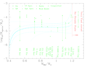
Figure 9: Nova ejected shell mass vs. mass of WD. The symbols describe the measured mass loss for different observed novae as compiled by Hack et al. (1993). Large measurement errors are apparent in cases where more than one measurement exists (in which case a vertical line connects the points). One should also note that some measurements overestimate the mass loss when the wind is clumpy, as it is predicted to be. The solid line describes the mass loss obtained by the wind model assuming a nominal value of ${\cal W}=10.0$ as obtained from Nova LMC 1988 #1, following the procedure given in the text. The long dashed line is obtained when changing the Hydrogen mass fraction from 0.7 to 0.3. The upper (and lower) short dashed lines are obtained when taking a value for ${\cal W}$ which is higher (lower) by 5.0, while the dash-dotted line arises when the assumed exponential decay is replaced by a linear decay. The dotted lines arise when taking into account the natural scatter in the $t_{3}$ – $M_{\mathrm{\mathrm{WD}}}$ relation obtained by Livio (1992).

To within the large uncertainties in the ejecta mass determinations (which have a $1-\sigma$ scatter of 0.54 dex), the prediction and observations appear to be in good agreement. The super-Eddington episode of novae could account for the bulk, if not all, of the ejected material as a function of $M_{\mathrm{WD}}$. One should nevertheless note that the logarithmic average of the observations: $\left<\log_{10}(M_{\mathrm{ejecta}}/M_{\sun}~{}{\mathrm{yr^{-1}}})\right>=-4.40\pm 0.09$ is on the upper side but still within the allowed region predicted by the SEW theory (which has only a small functional dependence on $M_{\mathrm{\mathrm{WD}}}$). Since some of the ejecta mass determinations are susceptible to clumpiness, taking the latter into account should tend to reduce the logarithmic average. If ${\cal C}\approx 3$ is a typical value and if characteristically about a half of the measurements actually measure $M_{\mathrm{ejecta}}{\cal C}$, then the average of the mass loss would be smaller by about a 0.25 dex.

Several additional conclusions can be drawn from Fig. 9. The plateau in the predicted mass loss, where the mass loss does not depend on the mass of the white dwarf, extends from $M_{\mathrm{WD}}=0.5M_{\odot}$ to $1.2M_{\odot}$. This appears to agree with observations. Moreover, the extrapolation to WD masses beyond $1.2M_{\odot}$ agrees with the mass loss observed from the very fast nova V1500 Cygni, however, this extrapolation should be done cautiously because the assumption of a steady state wind is not strictly valid.

The plateau predicted by the SEW and seen in the observations is counter to theoretical predictions of the TNR process in which the general trend should be a smaller mass loss with larger WD masses. This theoretical trend arises from the fact that more massive WDs are more compact and ignite the TNR after significantly less material is accreted. For some reason, this trend is not seen. The current TNR theory of novae tends to predict values which are about half an order to an order of magnitude smaller than the typical observations for large WD masses (e.g., [Starrfield, 1999], [Prialnik & Kovetz, 1995], [Starrfield et al., 1998]). The implementation of the SEW theory in numerical simulations of thermonuclear runaways in now underway with the purpose of finding the luminosity at the base of the wind self consistently as well as to see to what extent the incorporation of the SEW changes the predicted amount of ejected material.

3.9 A ‘Constant Bolometric Flux’

Let us return to Fig. 4. Recall that lines of constant radius are close to being vertical. One can see that for moderately ‘loaded’ winds and $\Gamma_{0}$ of a few, an evolution in which the temperature increases but the apparent luminosity remains constant is possible if the radius does not decrease dramatically. Under such conditions, the luminosity at the base of the wind does fall off to get a higher and higher temperature. However, the lower mass loss predicted implies that less energy is needed to accelerate the material to infinity and so a larger fraction of the base luminosity remains after the wind has been accelerated.

This could explain for example the constant bolometric luminosity observed for V1974 Cygni 1992 ([Shore et al., 1994]) and supports the early working hypothesis ([Bath & Shaviv, 1976], [Gallagher & Starrfield, 1976]) that novae evolve with a bolometric luminosity which is almost constant, or at least one that does not vary dramatically.

Interestingly, depending on the load of the wind, the constant apparent bolometric flux can be either super or sub-Eddington. That is, even if an apparent sub-Eddington luminosity is observed, the system could still have been super-Eddington over dynamically long durations. In such cases, the kinetic and potential energies of the flow are important players in the total energy budget.

3.10 Clumpiness of the wind

Clumpiness was already mentioned on several occasions. Since it is important, it deserves a more concentrated discussion.

SEWs are expected to be always clumpy as they are generated by an inhomogeneous atmosphere. The results for ${\cal C}^{0.67}{\cal W}$ for Nova FH Serpentis as compared to the results for ${\cal W}$ of Nova LMC 1988 #1 do indicate that the winds are clumpy and that the clumpiness factor could be similar to that already observed in the optically thick winds of Wolf-Rayet stars, namely, ${\cal C}\sim 3$. This can be seen in Fig. 10 which depicts the ${\cal W}$ obtained in the three discussed systems.

Figure 10: Comparison of the wind parameter obtained from three independent objects. In the case of FH Ser, the result ${\cal C}^{0.67}{\cal W}$ constitutes an upper limit since any clumpiness in the wind will mimic a larger inferred value for ${\cal W}$ if homogeneity (i.e., ${\cal C}=1$) is assumed. The value of ${\cal C}=3$ is a guesstimate from the clumpiness observed in WR winds. Since the wind is expected to be clumpy, the larger value obtained is a good indication that the analysis and the model are consistent. The vertical dotted lines describe the theoretical prediction and its uncertainties using the simple ‘blob’ model. For nominal values for the unknown geometrical parameters ($\alpha=1/2$, $\beta=1$ and $\Xi=2$), the central line is obtained using eqs. (17) and (29). The two additional dotted lines represent the uncertainties arriving from the geometrical parameter $\Xi$ describing the surface to volume ratio in units of the size of the blobs, which could reasonable vary from $\Xi\sim 1$ to $\Xi\sim 3$. The arrows represent the change in the predicted ${\cal W}$ when changing the volume fraction of the dense regions. When large volume asymmetry is present, the value of ${\cal W}$ increases. It is minimized for $\alpha=1/3$. $\beta$ can shift ${\cal W}$ in both directions. The dashed vertical line represents the prediction using the Markovian results (eq. 27). Clearly, the results from the three objects are consistent with each other. They are somewhat larger than the theoretical prediction using nominal values ($\beta=1$, $\alpha=1/2$) but they do agree with the predictions using geometrical parameters well within reasonable bounds (e.g., $\alpha\sim 0.8$ or larger).

Clumpiness is also important because it tends to offset the estimates for the mass ejected from novae and other objects by overestimating it. This arises because many emission processes are more efficient at higher densities. For example, the opacity per unit mass of free-free emission is proportional to $\rho$. Thus, if the material is clumpy, then the higher density material is more efficient in producing the observed radiation than the case of the material spread evenly over the entire volume.

What is the expected size of the clumps? Since they originate from the inhomogeneities at the base of the wind, one needs to know the typical size $d$ of the atmospheric perturbations at this point. For the instabilities found to operate in Thomson scattering atmosphere ([Shaviv, 2001]), the typical size is of the order of the size of the pressure scale height $l_{p}$ (say, $\beta l_{p}$). As the wind expands from its base, the clumps will keep their angular extent relative to the star. Thus, the spherical harmonic $\ell$ at which the structure should peek should be of order:

$$\ell\approx 2\pi{R\over d}=2\pi{R\over\beta l_{p}}\approx{\pi(1-\Gamma_{\mathrm{eff},\infty})\over\beta\nu}{v_{\mathrm{esc}}^{2}\over v_{s}^{2}},\quad\beta\sim{\cal O}(1)$$ (51)

where $v_{s}$ is the speed of sound at the base of the wind, which is higher than that at the photosphere. The typical number obtained for novae, is $\ell\sim 100$. This is a large number and it implies that the ejecta has many small clumps in it. Since the perturbations are expected to be dynamic and change over a sound crossing time, their vertical extent should be of order $(v_{\infty}/v_{s})\beta l_{p}$, at large distances, after the velocity dispersion had time to disperse the blobs vertically. The horizontal dispersion arising from velocities of order of the speed of sound are not important because of the horizontal expansion induced by rarefaction in the spherical geometry.

4 Discussion & Summary

The existence of steady state super-Eddington outflows is an observational fact. One therefore needs to explain on one hand how atmospheres can sustain a super-Eddington state and on the other, one needs to understand the winds that they generate.

We have tried to present the following coherent picture: Homogeneous atmospheres becomes inhomogeneous as the the radiative flux approaches the Eddington limit. This is due to a plethora of instabilities. The particular governing instability depends on the details of the atmosphere. As a consequence of the inhomogeneity, the effective opacity is reduced as it is easier for the radiation to escape, and consequently, the effective Eddington limit increases.

Super-Eddington configurations are now possible because the bulk of the atmosphere is effectively sub-Eddington so that the average is also sub-Eddington. Very deep layers advect the excess total luminosity above Eddington by convection. Higher in the atmosphere, where convection is inefficient, the Eddington limit is effectively increased due to the reduced effective opacity. The top part of the atmosphere, where perturbations of order of the scale height become optically thin, has however to remain super-Eddington. Thus, these layers are pushed off by a continuum driven wind.

By identifying the location of the critical point of the outflow, one can obtain a mass-loss luminosity relation. The relation, given by eq. (30) is the main result of the paper. Adding to eq. (30) the basic results for optically thick winds eq. (36) ([Owocki & Gayley, 1997]) and eq. (2.5) ([Bath & Shaviv, 1976]) or eq. (2.5) ([Bath, 1978]), we are left with one free universal dimensionless function ${\cal W}$. It was shown that ${\cal W}$ depends primarily on the geometrical characteristics of the inhomogeneous atmosphere from which the wind emerges. Having no detailed information on the geometrical properties, we assumed that they are independent of $\Gamma$, so that ${\cal W}$ becomes a constant.

To check these ideas, we analyze 2 novae as well as the massive star $\eta$ Carinae for which sufficiently detailed and accurate data is available. Although the two types of systems are notably different, as they have masses, luminosities and mass loss rates which differ by orders of magnitude, the wind mass loss and the wind parameter are found to be in agreement with the theoretical expectation:

$$\dot{M}={\cal W}{{\cal L}_{\mathrm{Edd}}\over cv_{s}}(\Gamma-1),~{}{\rm with}~{}{\cal W}=10.0\pm 5.$$ (52)

The evolution of the temperature predicted from the luminosity agrees well with the temperature measured directly in the two novae.

Another interesting agreement is the consistency with clumping. Clumping in SEWs is a natural prediction since the atmospheric layers beneath the sonic point are predicted to be inhomogeneous. Moreover, clumpiness is a necessary ingredient in the present theory that allows super-Eddington luminosities. The present theory predicts therefore, that SEWs are clumpy. In the analysis of Nova FH Serpentis, the wind parameter obtained is coupled to the clumpiness of the wind since a clumpy wind with the same observed colour temperature will have a lower inferred mass loss. The lower $\dot{M}$ reduces the measured wind parameter towards that obtained for Nova LMC 1988 #1 when the typical clumpiness factors seen in WR winds are taken into account.

The consistency of all the results is best demonstrated in Fig. 10 which shows that ${\cal W}$ obtained from the three different objects is consistent with one another. Although ${\cal W}$ obtained is somewhat larger than the theoretical prediction using nominal values for the geometrical characteristics, the uncertainties in the latter are large enough to comfortably accommodate the range of ‘measured’ ${\cal W}$’s.

An additional way of viewing the results is as follows. The SEW theory predicts a range of ${\cal W}$ which due to uncertainties can span at least an order of magnitude. The analysis of Nova LMC 1988 #1 yields a ${\cal W}$ which agrees with this range. The analysis of Nova FH Serpentis yields a ${\cal W}$ which too agrees with this range if clumpiness, which is predicted, is included. Next, instead of finding the values of ${\cal W}$ which best fit $\eta$ Car, we could have asked the opposite question. Using the SEW theory which was ‘normalized’ using Nova LMC 1988 #1, we could have calculated what the observed mass loss should have been according to the SEW theory, and find out that its prediction is completely consistent with the observed mass loss, even though the object’s characteristics are different from novae by several of orders of magnitude.

We also identify the occurrence of the ‘transition phase’ observed in more than two thirds of the novae with the advance of the atmosphere into the ‘no steady state region’. As the nova explosion progresses, its luminosity and radius decline. However, if the radius decreases too quickly, at some point the predicted SEW will be too heavy for the luminosity at the base to push mass to infinity. No steady state will then exist. The inconsistency might explain the strange behaviours observed in the transition phase of different novae.

The wind model presented is by no means a complete theory for novae since it cannot predict ab initio the luminosity at the base of the wind. To obtain the latter, one needs to solve for the complete evolution of a nova taking into account the fact that the nova’s atmosphere becomes porous and feels a reduced effective opacity. One expects that the lowered opacity increases the luminosity obtained in the core-mass luminosity relation, and super-Eddington values therefore arise naturally. Preliminary numerical solution of the stellar structure equations appear to confirm this prediction.

In order to fully understand the behaviour of the atmosphere that drives these winds, a 2D or even 3D numerical simulations on scales of the order of few optical depths are unavoidable because of the intrinsic nonlinear properties of the problem. These simulations are underway and will allow one to study in detail the physics controlling the mass outflow.

Appendix A The Effective opacity when not fully in the optically thick or thin limits

We proceed here to calculate the corrections to the effective opacity in systems which are neither fully in the optically thick limit nor fully in the optically thin limit. This analysis is presented to strengthen the heuristic arguments given in the section calculating the location of the critical point. It also depicts the problems arising when facing the task of calculating the radiation transfer in a nonlinear inhomogeneous medium. We begin with an analysis of a system that is not fully in the optically thick limit and continue with an estimating the effective opacity when not fully in the thin limit.

A.1 Regions close to the optically thick limit

Although it is apparently impossible to solve in a close analytical form the opacity reduction in an arbitrary nonlinear configuration, we attempt to solve it in at least one realistic configuration in order to estimate more accurately ${\cal B}$ and $p_{h}$. We shall now assume for simplicity that the perturbations are vertically elongated. This is actually a reasonable approximation because the unstable modes found in Shaviv ([Shaviv, 2001]) typically have $k_{x}\sim l_{p}^{-1}$ but a somewhat smaller $k_{z}$. This implies that most of the interface between high density and low density regions is vertical and that the isothermal contours are mostly horizontal.

Since the medium is close to the thick limit, we solve for the radiation in the vicinity of the interface, assuming that it is flat and the two density regions extend infinitely to either side.

The framed region shown in figure 2 corresponds to a typical area which we wish to solve. We assume that both sides of the region have $B=B_{0}+bz$. The dense region on the right has $\rho_{h}\equiv(1+\delta){\bar{\rho}}$ and the underdense on the left has $\rho_{l}\equiv(1-\delta){\bar{\rho}}$.

Using the formal solution given by eq. (19), we can write the radiation intensities. For points located in the high density region, at a horizontal coordinate $x_{0}$, the intensity for trajectories coming from the positive direction is given by:

$$I(x_{0},{\hat{\bf n}}_{-})\hskip-3.0pt = \hskip-3.0ptB_{0}+b\kappa_{0}{\bar{\rho}}{\tan\mu\cos\varphi\over\cos\mu}$$

$$\hskip-35.0pt\times\int_{x_{0}}^{\infty}(1+\delta)(x-x_{0})\exp\left[-{\kappa_{0}{\bar{\rho}}(x-x_{0})(1+\delta)\over\cos\mu}\right]dx,$$

where $\mu$ is the direction of the ray relative to the x-axis (perpendicular to the interface) such that $s=x/\cos\mu$ and $z=x\tan\mu\cos\varphi$. For trajectories coming from the negative x-direction, we have:

$$I({\bf x},{\hat{\bf n}}_{+})\hskip-5.0pt = \hskip-5.0ptB_{0}+b\kappa_{0}{\bar{\rho}}{\tan\mu\cos\varphi\over\cos\mu}$$

$$\hskip-55.0pt\hfill\times\left\{\int_{0}^{x_{0}}(1+\delta)(x-x_{0})\exp\left(-{\kappa_{0}{\bar{\rho}}(x-x_{0})(1+\delta)\over\cos\mu}\right)dx\right.$$

$$\hskip-55.0pt\hfill+\left.\hskip-3.0pt\int_{-\infty}^{0}\hskip-5.0pt(1-\delta)(x-x_{0})\exp\hskip-3.0pt\left[-{\kappa_{0}{\bar{\rho}}\left[x_{0}(1+\delta)+x(1-\delta)\right]\over\cos\mu}\right]\hskip-3.0ptdx\right\}.$$

This time $\cos\mu$ is negative. If we now integrate to get the flux, we find

$$F(x_{0}>0)\hskip-3.0pt = \hskip-3.0pt{4\pi b\over 3c\kappa_{0}{\bar{\rho}}(1+\delta)}+{\pi b\over 3c{\bar{\rho}}\kappa_{0}}(1-\delta^{2})$$

$$\hfill\hskip-55.0pt\times\left[{\tilde{x}_{0}}\delta(1+\delta)\left(-6+{\tilde{x}_{0}}^{2}(1+\delta)^{2})\Gamma(0,{\tilde{x}_{0}}(1+\delta))\right)\right.$$

$$\hskip-55.0pt\hfill+\left.\delta(-4+{\tilde{x}_{0}}(1+\delta)(-1+{\tilde{x}_{0}}+{\tilde{x}_{0}}\delta))\exp(-{\tilde{x}_{0}}(1+\delta))\right]$$

with ${\tilde{x}_{0}}\equiv x_{0}\kappa_{0}{\bar{\rho}}$. $\Gamma(n,x)$ is the incomplete $\Gamma$ function (and should not be confused with the Eddington parameter $\Gamma$). The first term is the uncorrected flux $F_{h}$ in the high density region while the rest of the expression is the correction near the interface with the low density region. The net correction to the average flux of the system from only corrections in the positive x-axis is:

$$\Delta F_{+}={S\over V_{\mathrm{tot}}}\int_{0}^{\infty}(F-F_{h})dx={\pi(S/V_{\mathrm{tot}})\delta^{2}\over 2c\kappa_{0}{\bar{\rho}}(1-\delta)(1+\delta)^{2}}.$$ (56)

The flux in the negative half, where the density is ${\bar{\rho}}(1-\delta)$ is obtained by the transformation $\delta\rightarrow-\delta$. The sum of the net correction to the flux on both sides of $x=0$ is the total correction to the average flux in the system:

$$\Delta F=\Delta F_{+}+\Delta F_{-}=-{\pi(S/V_{\mathrm{tot}})b\delta^{2}\over c\kappa_{0}{\bar{\rho}}(1-\delta^{2})^{2}}.$$ (57)

The average flux of the system, had it been homogeneous, is $F_{0}=4\pi b/3c\kappa_{0}\rho_{0}$. If we then assume $\Gamma\gg 1$ or $\delta\rightarrow 1$ and use eq. (12), we find:

$${\Delta F\over F_{0}}=\left(\kappa_{0}\over\kappa_{\mathrm{eff},\infty}\right)^{2}{3S\over 32\alpha(1-\alpha)^{2}\kappa_{0}\rho_{0}V_{\mathrm{tot}}}.$$ (58)

This result should be compared with the one obtained in the more heuristic treatment (eq. 14). The correction to the flux obtained here has an additional factor of $3/(8\alpha)$ but is otherwise the same. That is, if we compare $\kappa_{\mathrm{eff}}$ as given by eq. (2) with $\psi={\cal B}\Delta\tau^{-p_{h}}$, we obtain $p_{h}=1$ and ${\cal B}=(3\Xi/32\alpha(1-\alpha)^{2})/\beta$.

A.2 Regions close to the optically thin limit

We begin with systems approaching the thin limit. To calculate the radiation transfer we should perform a linear analysis in which the zeroth order terms are those of the thin limit. That is to say, the zeroth order terms are those arising when the optical depth of the perturbations can be neglected (even if $\delta\rho/\rho\sim{\cal O}(1)$).

The formal solution to the radiation transfer is given by eq. (19). It assumes that the boundaries are many optical depths away. This is valid also in the optically thin case because even if a scale height is optically thin, the generated wind is optically thick unless $\Gamma-1$ is extremely smaller than unity. We also implicitly assume that the photon crossing time is significantly shorter than any dynamical time scale in the system on which the perturbations can change their structure.

We write the radiation source function of the unperturbed region as $B_{0}(\bf{r})$ and the density as $\rho_{0}(\bf{r})$, while the corresponding perturbations are $B_{1}(\bf{r})$ and ${\rho_{1}(\bf{r})}$.

If we perturb the formal solution of the transfer equation (eq. 19) we find:

$$I_{0}({\bf x},{\hat{\bf n}}) = \int_{0}^{\infty}\chi_{0}B_{0}e^{-\chi_{0}s}ds$$ (59)

$$I_{1}({\bf x},{\hat{\bf n}}) \approx \int_{0}^{\infty}\chi_{0}B_{1}e^{-\chi_{0}s}ds+\int_{0}^{\infty}\chi_{1}B_{0}e^{-\chi_{0}s}ds$$

$$-\int_{0}^{\infty}\chi_{0}B_{0}e^{-\chi_{0}s}\left(\int_{0}^{s}\chi_{1}ds^{\prime}\right)ds.$$

The small parameter used for the expansion is $E_{1}\equiv\int_{0}^{s}\chi_{1}(s^{\prime})ds^{\prime}$, namely, the perturbation to the extinction $E$ which appears in the exponent. If $E_{1}$ is much smaller than unity, than $\exp(-E_{0}-E_{1})\approx\exp(-E_{0})(1-E_{1})$. Note that $E_{1}\ll 1$ for $s$’s of order the m.f.p of a photon or smaller.

Next, we assume for simplicity that the unperturbed radiation source function can be written as: $B_{0}({{\bf x}})=\bar{B}_{0}+{\bf x}\cdot{\bf b}$. After the linearization, it is meaningful to look for harmonic solutions to the equations of the form $X_{1}={\tilde{X}}_{1}e^{i{{\bf k}}\cdot{\bf x}}$ where $X_{1}$ is any perturbed quantity.

The expression for the first order perturbation to the specific intensity can then be obtained rather straightforwardly if we change the integration order for the double integral and choose an integration coordinate system in which ${\bf b}$ aligns with the $z$-axis (as opposed to aligning ${{\bf k}}$ with $z$). One then finds:

$$I_{1}({\bf x},{\hat{\bf n}})=\left({\chi_{0}B_{1}\over i{{\bf k}}\cdot{\hat{\bf n}}+\chi_{0}}+{1\over\chi_{0}}{({\hat{\bf n}}\cdot{\bf b})\chi_{1}\over i{{\bf k}}\cdot{\hat{\bf n}}+\chi_{0}}\right)e^{i{{\bf k}}\cdot{\bf x}}.$$ (60)

The first term describes changes in the source function due to local changes in the temperature. The second term describes changes in the optical depth due to temperature and density perturbations along the line of sight.

Once the expression for the perturbed radiative flux is known, the moments of $I$ can be evaluated directly from the perturbed radiation field. Starting with the lowest moment, $J$ is:

$$J_{1}({\bf x}) \hskip-3.0pt=\hskip-3.0pt {1\over 4\pi}\oint I_{1}({\bf x},{\hat{\bf n}})d{{\bf{\Omega}}}$$

$$\hskip-3.0pt=\hskip-3.0pt {1\over 4\pi}\left[\oint{\chi_{0}B_{1}d{{\bf{\Omega}}}\over i{{\bf k}}\cdot{\hat{\bf n}}+\chi_{0}}+{1\over\chi_{0}}\oint{({\hat{\bf n}}\cdot{\bf b})\chi_{1}d{{\bf{\Omega}}}\over i{{\bf k}}\cdot{\hat{\bf n}}+\chi_{0}}\right]e^{i{{\bf k}}\cdot{\bf x}}$$

$$\hskip-3.0pt=\hskip-3.0pt \left[\Lambda_{1}\left(k\over\chi_{0}\right)B_{1}-i{{{\bf k}}\cdot{\bf b}\over 3\chi_{0}^{2}}\Lambda_{2}\left(k\over\chi_{0}\right){\chi_{1}\over\chi_{0}}\right]e^{i{{\bf k}}\cdot{\bf x}}.$$

To obtain the last equality we choose the integration coordinate system so that ${{\bf k}}$ is parallel to its $z$-axis. In this particular choice the denominators of the integrals obtain their simplest form. We also defined the following three functions for convenience:

$$\begin{array}[c]{rclrcl}\Lambda_{1}(\xi)&\hskip-3.0pt\equiv\hskip-3.0pt&{1\over\xi}\tan^{-1}(\xi)&\Lambda_{1}(\xi\gg 1)&\hskip-3.0pt\approx\hskip-3.0pt&{\pi\over 2}{1\over\xi}\\ \Lambda_{2}(\xi)&\hskip-3.0pt\equiv\hskip-3.0pt&\left({3\over\xi^{2}}-{3\over\xi^{3}}\tan^{-1}(\xi)\right)&\Lambda_{2}(\xi\gg 1)&\hskip-3.0pt\approx\hskip-3.0pt&{3\over\xi^{2}}\\ \Lambda_{3}(\xi)&\hskip-3.0pt\equiv\hskip-3.0pt&{3\left[(\xi^{2}+1)\tan^{-1}(\xi)-\xi\right]\over 2\xi^{3}}&\hskip 6.0pt\Lambda_{3}(\xi\gg 1)&\hskip-3.0pt\approx\hskip-3.0pt&{3\pi\over 4}{1\over\xi}.\end{array}$$

The third function will be used shortly. The unperturbed value of $J$ is $J_{0}=\bar{B}_{0}$.

The first moment of $I$ is related to the flux (${\bf F}=(4\pi/c){{\bf H}}$) and given by:

$${{\bf H}}_{1}({\bf x}) \hskip-3.0pt=\hskip-3.0pt {1\over 4\pi}\oint I_{1}({\bf x},{\hat{\bf n}}){\hat{\bf n}}d{{\bf{\Omega}}}$$

$$\hskip-3.0pt=\hskip-3.0pt {1\over 4\pi}\left[\oint{\chi_{0}{\hat{\bf n}}B_{1}d{{\bf{\Omega}}}\over i{{\bf k}}\cdot{\hat{\bf n}}+\chi_{0}}+\oint{({\hat{\bf n}}\cdot{\bf b}){\hat{\bf n}}\chi_{1}d{{\bf{\Omega}}}\over i{{\bf k}}\cdot{\hat{\bf n}}+\chi_{0}}\right]e^{i{{\bf k}}\cdot{\bf x}}$$

$$\hskip-3.0pt=\hskip-3.0pt \left\{{{{\bf k}}\over 3i\chi_{0}}\Lambda_{2}\left(k\over\chi_{0}\right)B_{1}+{\chi_{1}\over 3\chi_{0}^{2}}({\bf b}\cdot{\hat{\bf k}}){\hat{\bf k}}\Lambda_{2}\left(k\over\chi_{0}\right)\hskip-3.0pt\right.$$

$$+\left.{\chi_{1}\over 3\chi_{0}^{2}}({\bf b}-({\bf b}\cdot{\hat{\bf k}}){\hat{\bf k}})\Lambda_{3}\left(k\over\chi_{0}\right)\right\}e^{i{{\bf k}}\cdot{\bf x}}$$

where ${\hat{\bf k}}$ is a unit vector in the direction of ${{\bf k}}$. The first term arises from perturbations to the temperature while the second and third from perturbations to the opacity.

When close to the Eddington limit, the region where the optical depth of a scale height is of order unity should be in the NAR limit (e.g., [Shaviv, 2001], [Glatzel & Kiriakidis, 1993]) unless the absorption opacity is extremely small (smaller than about $(p_{\mathrm{rad}}/p_{\mathrm{gas}})(v_{s}/c)$ times the ratio between the absorption opacity and the scattering opacity). Consequently, one can assume that heating or cooling of the gas is instantaneous and that $B=J$. If we impose $J_{1}=B_{1}$ (since the zeroth order terms satisfy it anyway), we find from eq. (A.2) that:

$$B_{1}=-{\Lambda_{2}\left(k\over\chi_{0}\right)\over 1-\Lambda_{1}\left(k\over\chi_{0}\right)}{i{{\bf k}}\cdot{\bf b}\over 3\chi_{0}^{2}}{\chi_{1}\over\chi_{0}}.$$ (63)

If we write $\xi\equiv\left(k/\chi_{0}\right)$ then the correction to the flux is:

$${{\bf H}}_{1}({\bf x}) \hskip-3.0pt=\hskip-3.0pt \left\{{{{\bf k}}\over 3\chi_{0}}{\Lambda_{2}^{2}(\xi)\over\Lambda_{1}(\xi)-1}{{{\bf k}}\cdot{\bf b}\over 3\chi_{0}^{2}}+{\chi_{1}\over 3\chi_{0}^{2}}({\bf b}\cdot{\hat{\bf k}}){\hat{\bf k}}\Lambda_{2}\left(\xi\right)\hskip-3.0pt\right.$$ (64)

$$+\left.{\chi_{1}\over 3\chi_{0}^{2}}({\bf b}-({\hat{\bf b}}\cdot{\hat{\bf k}}){\hat{\bf k}})\Lambda_{3}\left(\xi\right)\right\}e^{i{{\bf k}}\cdot{\bf x}}.$$

First, we note that the first two terms are proportional to $\xi^{-2}$ for large $\xi$’s or short wavelengths while the third term falls only as $\xi^{-1}$ such that it would dominate for low $\xi$’s. This fact provides the justification for neglecting the temperature perturbations in the heuristic picture given in §2.3. Moreover, careful analysis of the definition of the $\Lambda_{i}$’s will reveal that the first two terms actually cancel each other.

The effective opacity of the medium can now be calculated using Shaviv ([Shaviv, 1998]):

$$\chi_{\mathrm{eff}} = {\left<H\chi\right>\over\left<H\right>}={H_{0}\chi_{0}+\left<H_{1}\chi_{1}\right>+\left<H_{1}\right>\chi_{0}+H_{0}\left<\chi_{1}\right>\over H_{0}+\left<H_{1}\right>}$$ (65)

$$= {H_{0}\chi_{0}+\left<H_{1}\chi_{1}\right>\over H_{0}}$$

$$= {\chi_{0}}-{3\pi\over 8}{\chi_{1}^{2}\over\chi_{0}}({\hat{\bf z}}-({\hat{\bf z}}\cdot{\hat{\bf k}}){\hat{\bf k}}){\chi_{0}\over k}$$

where we have used the $\xi\gg 1$ expansion of $\Lambda_{3}$ and assumed without loss of generality that ${\bf b}$ is in the ${\hat{\bf z}}$ direction. We point out that had we worked with the opacity per unit mass $\kappa$ instead of the extinction $\chi$, which is the opacity per unit volume, the averaging $\left<\right>$ would have been a mass weighted average and not a volume average.

It would be interesting to solve the problem exactly in the same case which is solved for in the thick limit, namely, that of vertical slabs of width $d$ and a density of $\rho_{0}(1\pm\delta)$. To do so, we use the Fourier series expansion for the density:

$$\rho(x)=\rho_{0}\left(1+{4\delta\over\pi}\sum_{n=0}^{\infty}{\sin\left[(2n+1)\pi x/d\right]\over 2n+1}\right)$$ (66)

For Thomson atmospheres we find that $\chi_{1}=\kappa_{0}\rho_{1}$. If the identity $\sum_{n=0}^{\infty}1/(2n+1)^{3}=7\zeta(3)/8$ is used (with $\zeta(x)$ being the $\zeta$-function), we obtain:

$${\kappa_{\mathrm{eff}}\over\kappa_{0}}={\chi_{\mathrm{eff}}\over\chi_{0}}=1-{21\zeta(3)d\kappa_{0}\rho_{0}\over 2\pi^{2}}\delta^{2}\approx 1.28d\kappa_{0}\rho_{0}\delta^{2}.$$ (67)

We can also write $\delta^{2}=(\kappa_{0}-\kappa_{\mathrm{eff},\infty})/\kappa_{0}$ in the case of vertical slabs. If we now compare this result to eq. (2), with $\psi(\Delta\tau\ll 1)\approx 1-\Delta\tau^{p_{l}}$, we obtain: $p_{l}=1$ and ${\cal A}\approx 1.28d\kappa_{0}\rho_{0}/\Delta\tau=1.28\beta$.

In the more general case of $\alpha\neq 1/2$, an analytic solution does exist but it involves poly-logarithm functions of $\alpha$ which would appear in ${\cal A}$, changing it by ${\cal O}(1)$.

References

- Arons, 1992 Arons J., 1992, ApJ, 388, 561
- Bath, 1978 Bath G. T., 1978, MNRAS, 182, 35
- Bath & Shaviv, 1976 Bath G. T., Shaviv G., 1976, MNRAS, 175, 305
- Castor et al., 1975 Castor J. I., Abbott D. C., Klein R. I., 1975, ApJ, 195, 157
- Davidson, 1999 Davidson K., 1999, in Morse J. A., Humphreys R. M., Damineli A., eds, ASP Conf. Ser. 179: Eta Carinae at The Millennium, p. 6
- Davidson & Humphreys, 1997 Davidson K., Humphreys R. M., 1997, ARA&A, 35, 1
- della Valle et al., 1997 della Valle M., Gilmozzi R., Bianchini A., Esenoglu H., 1997, A&A, 325, 1151
- Duerbeck, 1992 Duerbeck H. W., 1992, Acta Astronomica, 42, 85
- Friedjung, 1987 Friedjung M., 1987, A&A, 179, 164
- Friedjung, 1989 Friedjung M., 1989, in Bode M. F., Evans A., eds, Classical Novae, John Wiley & Sons, Oxford
- Gallagher & Code, 1974 Gallagher J. S., Code A. D., 1974, ApJ, 189, 303
- Gallagher & Starrfield, 1976 Gallagher J. S., Starrfield S., 1976, MNRAS, 176, 53
- Gill & O’Brien, 2000 Gill C. D., O’Brien T. J., 2000, MNRAS, 314, 175
- Glatzel & Kiriakidis, 1993 Glatzel W., Kiriakidis M., 1993, MNRAS, 262, 85
- Hack et al., 1993 Hack M., Selvelli P., Duerbeck H. W., 1993, Cataclysmic Variables and Related Objects (N95-27068 09-89), NASA, Washington, p. 261
- Joss et al., 1973 Joss P. C., Salpeter E. E., Ostriker J. P., 1973, ApJ, 181, 429
- Kato & Hachisu, 1994 Kato M., Hachisu I., 1994, ApJ, 437, 802
- Levermore et al. (1986) Levermore, C. D., Pomraning, G. C., Sanzo, D. L., & Wong, J. 1986, Journal of Mathematical and Physical Sciences, 27, 2526
- Levermore et al. (1988) Levermore, C. D., Wong, J., & Pomraning, G. C. 1988, Journal of Mathematical and Physical Sciences, 29, 995
- Livio, 1992 Livio M., 1992, ApJ, 393, 516
- Mihalas & Weibel Mihalas, 1984 Mihalas D., & Weibel Mihalas B. 1984, Foundations of radiation hydrodynamics, Oxford univ. press, Oxford
- Owocki & Gayley, 1997 Owocki S. P., Gayley K. G., 1997, in Nota A., Lamers H., eds, ASP Conf. Ser. 120: Luminous Blue Variables: Massive Stars in Transition, p. 121
- Paczynski, 1970 Paczynski B., 1970, Acta Astronomica, 20, 47
- Paresce et al., 1995 Paresce F., Livio M., Hack W., Korista K., 1995, A&A, 299, 823
- Pauldrach et al., 1986 Pauldrach A., Puls J., Kudritzki R. P., 1986, A&A, 164, 86
- Pomraning (1992) Pomraning, G. C., 1992, Linear Kinetic Theory and Particle transport in Stochastic Mixtures, Series on Advances in mathematics for Applied Sciences, Vol. 7, Singapore: World Scientific, §3.4
- Prialnik, 1986 Prialnik D., 1986, ApJ, 310, 222
- Prialnik & Kovetz, 1995 Prialnik D., Kovetz A., 1995, ApJ, 445, 789
- Schwarz et al., 1998 Schwarz G. J., Hauschildt P. H., Starrfield S., Whitelock P. A., Baron E., Sonneborn G., 1998, MNRAS, 300, 931
- Schwarz et al., 2000 Schwarz, G. J., Shore, S. N., Starrfield, S., Hauschildt, P. H., Della Valle, M., & Baron, E. 2001, MNRAS, 320, 103
- Shaviv, 1998 Shaviv N. J., 1998, ApJ, 494, L193
- Shaviv, 2000 Shaviv N. J., 2000, ApJ, 532, L137
- Shaviv, 2001 Shaviv N. J., 2001, ApJ, 549, 1093
- Shore et al., 1994 Shore S. N., Sonneborn G., Starrfield S., Gonzalez-Riestra R., Polidan R. S., 1994, ApJ, 421, 344
- St.-Louis et al., 1993 St.-Louis N., Moffat A. F. J., Lapointe L., Efimov Y. S., Shakhovskoj N. M., Fox G. K., Piirola V., 1993, ApJ, 410, 342
- Starrfield, 1999 Starrfield S., 1999, Phys. Rep., 311, 371
- Starrfield et al., 1998 Starrfield S., Truran J. W., Wiescher M. C., Sparks W. M., 1998, MNRAS, 296, 502
- Stothers & Chin, 1993 Stothers R. B., Chin C., 1993, ApJ, 408, L85
- Tuchman et al., 1983 Tuchman Y., Glasner A., Barkat Z., 1983, ApJ, 268, 356
- Tuchman & Truran, 1998 Tuchman Y., Truran J. W., 1998, ApJ, 503, 381
- Warner, 1989 Warner B., 1989, in Bode M. F., & Evans A., eds, Classical Novae. John Wiley & Sons, Oxford