Abstract

The first generation of long-baseline laser interferometric detectors of gravitational waves will start collecting data in 2001–2003. We carefully analyse their planned performance and compare it with the expected strengths of astrophysical sources. The scientific importance of the anticipated discovery of various gravitatinal wave signals and the reliability of theoretical predictions are taken into account in our analysis. We try to be conservative both in evaluating the theoretical uncertainties about a source and the prospects of its detection. After having considered many possible sources, we place our emphasis on (1) inspiraling binaries consisting of stellar mass black holes and (2) relic gravitational waves. We draw the conclusion that inspiraling binary black holes are likely to be detected first by the initial ground-based interferometers. We estimate that the initial interferometers will see 2–3 events per year from black hole binaries with component masses 10–15 M_⊙, with a signal-to-noise ratio of around 2–3, in each of a network of detectors consisting of GEO, VIRGO and the two LIGOs. It appears that other possible sources, including coalescing neutron stars, are unlikely to be detected by the initial instruments. We also argue that relic gravitational waves may be discovered by the space-based interferometers in the frequency interval $2\times 10^{-3}$ Hz–$10^{-2}$ Hz, at the signal-to-noise ratio level around 3.

¹ Cardiff University, P.O. Box 913, Cardiff, CF2 3YB, U.K.
² Physics Department, Moscow University, 117234 Moscow, Russia
³ Sternberg Astronomical Institute, Moscow University, 119899 Moscow, Russia
e–mail:
L. P. Grishchuk: grishchuk@astro.cf.ac.uk V. M. Lipunov: lipunov@sai.msu.ru K. A. Postnov pk@sai.msu.ru M. E. Prokhorov mike@sai.msu.ru B. S. Sathyaprakash B.Sathyaprakash@astro.cf.ac.uk

1 Introduction

The goal of this review article is quite ambitious. We want to foretell the first gravitational wave signals that will be seen by sensitive detectors, several of which are currently in the final stage of construction. The detectors will start collecting data in a couple of years from now. Obviously, we present a subjective point of view. It is based on our evaluation of what we consider the best theoretical knowledge available today, in conjunction with the expected sensitivity of the instruments. Possibly, other authors would regard other sources more promising, and would place their bet on something else. It is also possible that our view is biased, because it is partially guided by the work that we personally were involved in. We will not be very disappointed if we are proved wrong. Nature may have many surprises in store for us. It is important, however, that for the first time in the long history of gravitational wave research, the conservative astrophysical estimates overlap with the detecting capabilities of real instruments. It is an appropriate time to prepare strategies for the search and analysis of signals that appear to be more probable than others.

The general theory of gravitational radiation is well understood and is described in textbooks [1, 2, 3]. The status of the gravitational wave astronomy has been regularly reviewed [4, 5, 6], including papers in Uspekhi [7, 8, 9, 10]. Here, we will only remind the reader that the gravitational waves are an inescapable consequence of Einstein’s general relativity and, indeed, of any gravitational theory which respects special relativity. Gravitational waves are similar to electromagnetic waves in several aspects. They propagate with the velocity of light $c$, have two independent transverse polarisation states, and in their action on masses have analogs of electric and magnetic components. Gravitational waves carry away from the radiating system its energy, angular momentum, and linear momentum. The gravitational–wave field is dimensionless, and its strength is qualitatively characterized by a single quantity — the gravitational wave amplitude $h$. The amplitude falls off in course of propagation from a localized source, in proportion to the inverse power of the traveled distance: $h\propto 1/r$. The difficulty of direct detection of gravitational waves can be seen from the fact that the expected amplitude $h$ on Earth from realistic astronomical sources is exceedingly small, of the order or smaller than $10^{-21}$. The conceivable amplitudes from laboratory sources are even smaller than that. This small number $h$ enters any possible scheme of detection of gravitational waves and makes the detection difficult to achieve. For instance, gravitational waves cause a tiny variation $\Delta l$ of the distance $l$ between two free masses: $\Delta l=hl$. In an interferometer with a 1 km arm-length the variation of the distance between the two end-mirrors would be of the order $\Delta l=10^{-16}~{}$cm. This tiny variation is supposed to be measured and distinguished against background noise. However, in the cosmos, gravitational waves are an important factor of cosmic evolution. Gravitational waves are routinely taken into account in the study of orbital evolution of close pairs of compact stars [11]. The measured secular change of orbital parameters in the binary system of neutron stars, which includes the pulsar PSR 1913+16, agrees with the gravitational wave prediction of general relativity to within 1% accuracy [12]. For the study of pulsars and this discovery, Hulse and Taylor were awarded a Nobel prize in 1993.

Like any other observational science, gravitational wave astronomy operates with sources, detectors, data analysis, and interpretation. In what follows, we devote some discussion to each of these notions. However, we are not aimed at reviewing all interesting astrophysical theories and all possible signals and detection techniques. We concentrate on sources, which, we believe, rest on the most solid theoretical foundation, are scientifically important, and involve minimal number of additional hypotheses. To be interesting from the point of view of its detection, the source should be sufficiently powerful, should fall in the frequency band of the detector, and occur reasonably often during the life-time of the instrument. The frequency range of the discussed signals is determined by the frequency intervals of the detectors’s sensitivity. The currently operating bar detectors are sensitive at frequencies around $10^{3}$ Hz. The ground-based laser interferometers are sensitive in the interval 10 Hz – $10^{4}$ Hz. The space-based laser antennas will be sensitive in the interval $10^{-4}$ Hz – 1 Hz. The great expectations are related with the forthcoming sensitive instruments. The Japanese scientists have already built a 300 m laser intergerometer called TAMA. The British-German collaboration is in the phase of completion of a 600 m laser interferometer called GEO600 [13]. The French-Italian collaboration is building a 3 km interferometer called VIRGO [14].The American project LIGO is building two 4 km arm-length interferometers [15]. It is expected that these instruments will become operational in 1–2 years. The proposal to build a Laser Interferometer Space Antenna (LISA) [16] has been tentatively approved by the European Space Agency and NASA, and the launch may occur around the year 2010. There exists also plans for advanced ground-based interferometers, such as LIGO-II [17].

The ability of a given instrument to detect a signal depends on the nature of the signal. The burst sources, which accompany cosmic catastrophes, emit gravitational radiation at some characteristic frequency during just a few cycles. They have tendency to be inherently powerful, but their event rate is very low. It is very unlikely to expect such an event to happen in our own Galaxy during, say, a 1–year observational run. To see a few events per year, one needs to survey a large (cosmological) volume of space and, hence, to possess a sensitive instrument capable of detecting the sources from the edges of this volume. The quasi-periodic astrophysical sources are expected to be more frequent than the burst sources, but they produce much weaker signals in terms of $h$. However, the amount of the radiated energy during some long time $T$ may be not much smaller than that of a burst source. If one knows, or can model, the temporal structure of the signal, one can monitor the detector’s output during many cycles that are covered by the observation time $T$. This can make a weak periodic signal not much more diffucult to detect than a burst signal. Some rare but reliable astrophysical sources, such as binary neutron stars and black holes at their latest stage of evolution, exhibit a kind of quasi-periodic gravitational wave signal at the inspiral phase, and more like a burst signal in the last moments of their coalescence and merging. The stochastic backgrounds of gravitational waves are typically weak and difficult to distinguish from the instrumental noise. However, if one can cross-correlate the outputs of two or more instruments, and can do this during a long integration time, the stochastic background can also be measured. The fundamentally important relic gravitational waves form a sort of a stochastic background. They are the only direct probe of the evolution of the very early Universe, up to the limits of the Planck era and Big Bang. It would be extremely valuable, even if difficult, to detect relic gravitational waves.

The balance between the expected scientific payoff and theoretical likelihood of various astrophysical sources versus their detectability by the forthcoming and planned instruments is the major thrust of this paper. After having analysed many possible sources of gravitational waves, and taking all the factors into account, we place our emphasis on compact binaries (neutron stars and black holes) and relic gravitational waves. In fact, we argue that inspiraling black holes, formed as a result of stellar evolution, are the most likely sources to be seen first by the forthcoming sensitive instruments. Also, we think that relic gravitational waves are likely to be detected by the advanced ground-based and space-based laser interferometers. To justify our point we go into a great detail in describing compact binary stars and relic gravitons.

Section 2 is devoted to the formation and evolution of binary systems. Binary stars are as numerous as single stars. Binaries emit gravitational radiation at twice their orbital frequency. To radiate gravitational waves with large intensity and at frequencies accessible to ground-based interferometers, the objects forming a pair should be massive and should orbit each other at very small separations — a few hundred kilometers. According to the existing views, these massive objects can only be the end-products of stellar evolution — neutron stars and black holes. Because of the loss of the angular momentum due to gravitational waves, these binary objects are in the late thousands of cycles at their inspiral phase. They are only tens of minutes away from the final coalescence and merging, or, possibly, from another spectacular event, a gamma–ray burst. The central question is how many such close systems exist in our Galaxy and at cosmological distances. This determines the event rate — the number of coalescence events that can occur in a given volume of space during, say, 1 year. A detector, sensitive enough to see the most distant objects in this volume, will detect all of them. A detector of lower sensitivity is capable of seeing the coalescing systems at shorter distances and, hence, will register a smaller number of such systems, or will not be expected to see them at all during a 1–year interval of observation.

In sub-section 2.1 we review all the observational data on binary neutron stars. Even these data alone, allow one to derive some estimates on the rate of neutron star coalescences. So far, there is no observational evidence of binaries consisting of a neutron star and a black hole or two black holes. However, we certainly do not see all the products of stellar evolution in binary systems. We need to take into account the predicitons of a theory which successfuly explains the formation and relative abundance of various populations of observed binaries consisting of normal stars and neutron stars. Such a theory predicts the existence of close binaries involving neutron stars and black holes, as the outcomes of processes along certain channels of the binary evolution. It is these channels of evolution that are most important for gravitational wave astronomy.

The sub-section 2.2 is devoted to the population synthesis method of describing the continuing birth and future fate of binary stars. The purpose of this analysis is to find the statistically expected number of massive and sufficiently close binaries, which could be in their final stage of inspiral at the present cosmological time. This means that we are interested only in those binaries whose expected total life-time, from formation to coalescence, is shorter than the Hubble time. As usual, the results of evolution depend on initial conditions and on physical processes along the evolutionary path. We combine the well-established observational facts with reasonable theoretical assumptions. Two parameters are especially important — the kick velocity ${\mathbf{w}}$ imparted to a newly born neutron star during a supernova explosion, and the fraction $k_{BH}$ of a pre-collapse massive star that goes into a resulting black hole. The formation of a black hole can also be accompanied by the impartation of some kick velocity. A large kick velocity can either disrupt a binary system — a would-be powerful source of gravitational waves, or, on the contrary, to make the binary orbit more eccentric, thus increasing the gravitational wave luminosity. In our evolutionary calculations we vary ${\mathbf{w}}$ and $k_{BH}$ in the observationally allowed limits. We also take into account the stellar wind and the loss of mass as factors of binary evolution. The kick velocity is so important a factor of binary evolution that we devote to its analysis a separate sub-section 2.3.

The results of the population synthesis are summarised in Section 3. These results are at the same time our predictions for the detection rate of various compact binary inspiral signals. In a given cosmological volume of space, the estimated event rate for coalescing black holes is about 10 times lower than that for coalescing neutron stars and neutron star – black hole systems. However, since the masses of black holes are significantly larger than the masses of neutron stars, they are more luminous gravitational wave sources than pairs of neutron stars. Hence, a given detector can observe inspiralling black holes at greater distances than pairs of inspiralling neutron stars. We conclude that a network of initial laser interferometers are likely to see black hole inspirals more often than the neutron star inspirals, and as often as 2–3 events per year.

Section 4 is devoted to transient and periodic sources. They include supernovae explosions, various unstable modes in rapidly rotating neutron stars, and quasi-normal modes of black hole perturbations. All these sources are interesting and potentially detectable. However, we do not place them at the beginning of our priority list. The asymmetric supernovae explosions, as well as the merging event of binaries can produce powerful bursts of gravitational radiation, but the estimates of their performance rely on factors which are not well understood theoretically and do not have much of observational evidence. The merging event will be probably seen as a confirming signature of the inspiral phase, but one cannot rely on this event alone. However, if we err in our priorities, a special kind of hypernovae explosions can top the list. As for the unstable modes in rotating neutron stars, they require quite sophisticated mechanisms of their excitation and can be hampered by viscosity and other physical processes. The collision of black holes and quasi-normal modes of newly born black holes is an intriguing possibility, but should probably be treated as something to be discovered by gravity wave observations, rather than reliably calculated on purely theoretical grounds.

In Section 5 we review stochastic gravitational wave backgrounds of astrophysical origin. These are the overlaping signals from many individual sources. The populations of sources that we consider include unresolved binary white dwarfs in our Galaxy and at cosmological distances, and the population of rotating neutron stars. The detection of these backgrounds would carry some scientific information on its own, but it is also necessary to study these sources for another reason. These stochastic backgrounds set a confusion limit for detection of more interesting signals by space-based and ground-based interferometers. We conclude that the LISA will be free of the gravitational wave noise from unresolved binaries at frequencies near and higher than $2\times 10^{-3}$ Hz. This noise is mostly from unresolved binaries in our Galaxy, the extra-Galactic binaries contribute only about 10% to this noise. Any detected stochastic background at frequencies above $2\times 10^{-3}$ Hz in the LISA window of sensitivity is expected to be of primordial origin. The population of non-axisymmetric rotating neutron stars could potentially blur the view of the ground-based interferometers. However, we find that this background is below the instrumental noise of initial interferometers, and can possibly present a problem only for the advanced LIGO. We estimate that other stochastic backgrounds of astrophysical origin are weaker than those that we have considered.

Section 6 is devoted to relic gravitational waves. In contrast to all other sources, which are based on classical physics, the generation mechanism of relic gravitons includes some elements of quantum physics. It is the inevitable zero-point quantum oscillations of gravitational waves amplified by the strong, variable gravitational field of the early Universe that ends up in a stochastic background of relic gravitational waves measurable today. Despite the fact that the existence of this gravitational wave signal involves an extra element — quantum physics, it is not less reliable than many other sources. The generation of relic gravitons relies essentially only on the validity of general relativity and basic principles of quantum field theory. Since the same mechanism is thought to be responsible for the generation of primordial density perturbation seeding the formation of galaxies, we present a qualitative picture of this mechanism in sub-section 6.1. The calculation of the expected relic gravitational wave background is given for a class of cosmological models supported by other observations. In particular, we use the data on the measured microwave background anisotropies. The results of this analysis are presented in sub-section 6.6. We find that in the most favorable case, the detection of relic gravitational waves can be achieved by the cross-correlation of outputs in the initial ground-based laser interferometers. In the more realistic case, the sensitivity of the advanced ground-based and space-based instruments will be needed. We also discuss a specific statistical signature of relic gravitons, associated with the phenomenon of squeezing. This phenomenon is also known in formal quantum mechanics and quantum optics. The signature of squeezing could potentially help in further improving the signal-to-noise ratio (SNR).

The problems of detectability are systematically referred to throughout the paper. However a rigorous discussion of detectors and data analysis is concentrated in Section 7 and Section 8. Whenever we qualify a source as detectable or undetectable, we base our conclusions on the more detailed treatment of these Sections. Section 7 gives a general description of detectors and their sensitivity curves. The important notion in the detection of a signal with a known or suspected temporal structure, is the notion of a template. A template allows one to use the mathched filtering technique (sub-section 8.1) in order to increase the SNR. This method will be indispensable in the search for signals from inspiraling binaries. The related issues are the practically accesible number of templates, their overlap in the parameter space, the computational cost, etc. These issues are important not only for a confident detection of a signal, but also for the extraction of astrophysical information from a signal (sub-sections 8.4–8.5) — the ultimate purpose of the gravitational wave astronomy.

Some mathematical details on the Keplerian motion of a binary system and gravitational reaction force are described in Appendix A1. Appendix A2 contains some technical issues of the mass transfer modes and mass loss in binary stars. Appendix A3 gives post-Newtonian expressions for energy and gravitational wave flux. The main conclusions of the review are formulated in the Abstract.

2 Astrophysical sources. Close binary neutron stars and black holes.

In this Section we discuss observational and theoretical estimates for the coalescence rate of close binary neutron stars and black holes. We start from a review of observational limits on the coalescence rate of binary neutron stars. Then, we describe the basics of the population synthesis of binary evolution which allows one to predict theoretically the event rates for systems involving neutron stars and black holes. The role of the kick velocity in the binary evolution is discussed in subsection 2.3. The expected detection rates in the forthcoming sensitive gravitational wave detectors are summarised in Section 3.

2.1 Observational limits on the binary neutron star coalescence rate

What do we know about compact binary stars and the rate of their mergings on observational grounds? More than a thousand of single neutron stars (NS) are currently (6)observed as radio-pulsars (see [18]; new data are being continuously added at http://puppsr.princeton.edu). In addition, about 30 NS are seen as X-ray pulsars and yet more 100 NS are seen as burst and transient X-ray sources. These NS enter binary systems with non-degenerate companions, that is, their companions are normal stars rather than neutron stars or black holes. Only six NS are known to enter binary systems with another NS as a secondary component . All these six systems belong to binary radio-pulsars. The systems and some of their parameters are listed in Table 1. Orbital periods are given in days and masses in units of the solar mass $M_{\odot}$. Three of these systems (namely, B1913+16, B1534+12 and B2127+11c) are close enough to merge due to GW emission in a time interval shorter than the Hubble time $t_{H}$. We loosely refer to binaries as coalescing or merging binaries if their expected life-time up to coalescence, $t_{coal}$, is shorter than $t_{H}$. For numerical estimates we use the value $t_{H}\simeq 12{\rm Gyr}=12\times 10^{9}{\rm yr}$.

Much less is known about black holes (BH). A dozen of BH candidates participate in binary systems with non-degenerate companions. They are observed as persistent X-ray sources (like Cyg X-1) or X-ray transients (mostly X-ray Novae) (see [21] for a review). Neither single BH nor BH forming a binary with radio-pulsar or another BH have been found so far. Parameters of the BH candidates in binary systems are listed in Table 2. Note that according to these data, the mean BH mass is $M_{\rm BH}\simeq 8.5M_{\odot}$, i.e. notably higher than a typical NS mass $M_{\rm NS}\simeq 1.4M_{\odot}$. (Of course, we mean a black hole in astrophysical sense, i.e. as a highly compact gravitating object of certain mass. The presence or absence of the event horizon is irrelevant for our discussion.) For a recent summary of NS mass determination see [22].

Table 1: Binary PSR with NS secondaries (data from [23])

PSR	$P_{b}(d)$	$e$	$M_{1}+M_{2}$	$M_{1}$	$M_{2}$	$t_{coales}$, yr
J1518+4904	8.634	0.249	2.62	$\ldots$	$\ldots$	$\geq$$3.6\,10^{12}$
B1913+161	0.323	0.617	2.8284	1.44	1.39	$1.0\,10^{8\ }$
B1534+121	0.420	0.274	2.6784	1.34	1.34	$1.0\,10^{9\ }$
B2127+11c1, 2	0.335	0.681	2.712	1.35	1.36	$8.0\,10^{7\ }$
B2303+46	12.340	0.658	2.60	$\ldots$	$\ldots$	$\geq$$1.6\,10^{12}$
B1820-113	357.762	0.795				$\mathrel{\mathchoice{\vbox{\offinterlineskip\halign{\hfil$\displaystyle#$\hfil\cr>\cr\vskip 1.5pt\cr\sim\cr}}}{\vbox{\offinterlineskip\halign{\hfil$\textstyle#$\hfil\cr>\cr\vskip 1.0pt\cr\sim\cr}}}{\vbox{\offinterlineskip\halign{\hfil$\scriptstyle#$\hfil\cr>\cr\vskip 0.5pt\cr\sim\cr}}}{\vbox{\offinterlineskip\halign{\hfil$\scriptscriptstyle#$\hfil\cr>\cr\vskip 0.5pt\cr\sim\cr}}}}$$2.4\,10^{15}$
1 Coalescing binary pulsars
2 Binary pulsar in a globular cluster
3 The secondary companion may not be a NS

Table 2: BH Candidates [21].

System Spectral class $P_{orb}$, d $f_{v}(m),M_{\odot}$ $m_{x},M_{\odot}$ $m_{v},M_{\odot}$ Cyg X-1 O9,7 Iab 5.6 0.23 7–18 20–30 LMC X-3 B(3–6)II–III 1.7 2.3 7–11 3–6 LMC X-1 O(7–9)III 4.2 0.14 4–10 18–25 A0620-00 K(5–7)V 0.3 3.1 5–17 $\sim$0.7 GS2023+338 K0IV 6.5 6.3 10–15 0.5–1.0 GSR1121-68 K(3–5)V 0.4 3.01 9–16 0.7–0.8 GS2000+25 K(3–7)V 0.3 5.0 5.3–8.2 $\sim$0.7 GRO J0422+32 M(0–4)V 0.2 0.9 2.5–5.0 $\sim$0.4 GRO J1655-40 F5IV 2.6 3.2 4–6 $\sim$2.3 XN Oph 1977 K3 0.7 4.0 5–7 $\sim$0.8 Cyg X-3 ? Mean Value of the BH mass $\sim$8.5M_⊙

There are two types of estimates of the binary NS coalescence rate. The estimates of the first type are derived directly from observations (see Table 3), while the estimates of the second type are inferred from theory of binary stellar evolution (see Table 4). We will consider each of these estimates in turn.

Table 3: Observational estimates of binary NS coalescence rate.

Author(s)	Coalescence rate (yr-1)
Phinney 1991 [24]	$1/10^{6}$
Narayan et al 1991 [25]	$1/10^{6}$
Curran, Lorimer 1995 [26]	$3/10^{6}$
van den Heuvel, Lorimer 1996 [27]	$8/10^{6}$
“Bailes limit” 1996 [28]	$<1/10^{5}$
Arzoumanian et al. 1999 [29]	$<1/10^{4}$

The estimates of the first type are based on the data on three binary radio-pulsars which should merge within the Hubble time (Table 1). These estimates use the following argumentation. The average coalescence time for these pulsars is approximately $3\times 10^{8}$ years. So the binary NS merging rate based on these 3 pulsars would be approximately once per 100 million years. As we observe only about 1% of the Galactic volume, a lower limit for the binary NS merging rate becomes one every million years [24]. In fact, this estimate was formulated at the time when only two of the presently known three coalescing binary radio-pulsars were known. Taking into account the spatial distribution of pulsars inside the Galaxy and the fact that a typical radiopulsar switches-off long before the coalescence, the lower limit for NS merging rate can be increased by almost an order of magnitude [27], thus reaching $10^{-5}$ per year.

An interesting upper limit, the so-called “Bailes limit”, was derived from independent arguments [28]. It was noted that the properties of the pulsars in the three coalescing binary radio pulsars (most of all, their surface magnetic fields) are quite different from those found in ordinary single radio pulsars. Since the number of single radio pulsars is about 1000, it is estimated that the radio pulsars similar to those residing in merging binary NS should be formed al least $\sim 1000$ times rarer than single radio pulsars. Taking the birth rate of single pulsars from a large sample of known pulsars, Bailes proposed to put an upper bound on the birth rate of binary NS as the (formation rate of single pulsars)$\times$ (number of pulsars with ordinary properties among binary radio-pulsars) = (1/60 yr)$\times$(1/1000)$\simeq 2\times 10^{-5}\,$yr^-1.

One should note, however, that in both the estimates – the one based on statistics of coalescing binary radio pulsars, and the other based on the Bailes’ limit – suffer from selection effects. They depend on the pulsar distances (in some cases known not better than up to a factor of 2) , on the characteristic pulsar life-time (known not better than up to an order of magnitude), and on the differences in the properties of single and binary pulsars. So, one cannot infer from observations an absolutely reliable estimate of the binary NS merging rate. Indeed, a recent re-assessment of the Bailes limit [29] taking into account the current pulsar numbers and the reduction in search sensitivity to short orbital period binaries gave $10^{-4}$ yr^-1 for the upper limit of binary NS Galactic merging rate. An alternative way of deriving the upper limit based on empirical pulsar birth rate and theoretical understanding of binary NS formation was used in [31] to yield a few mergers per $10^{5}$ years. The cited papers clearly demonstrate that (1) there is a steady tendency to increase the empirical upper limit of the binary NS coalescence rate and (2) various selection effects generic to radio pulsar surveys and lack of detailed knowledge of Galactic pulsar population properties still prevent us from the derivation of a fully reliable estimate.

2.2 Population synthesis of coalescing binary NS and BH

Now we turn to estimates partially based on theoretical grounds. The merging rates of binary compact stars have been calculated by different independent research groups, mostly with the help of the population synthesis numerical simulations (see Table 4). The reliability of these results depend on whether the binary evolution scenarios properly reflect different aspects of the real, observed populations. It is encouraging that these independent calculations yield similar results.

Table 4: Theoretical estimates of binary NS coalescence rate.

Author(s)	Coalescence rate (yr-1)
Clark et al 1979 [32]	$1/10^{4}$–$1/10^{6}$
Lipunov et al 1987 [33]	$1/10^{4}$
Hills et al 1990 [34]	$1/10^{4}$
Tutukov, Yungelson 1993 [35]	$3/10^{4}$–$1/10^{4}$
Lipunov et al 1995 [36]	$<3/10^{4}$
Portegies Zwart, Spreeuw 1996 [37]	$3/10^{5}$
Lipunov et al 1996 [38]	$3/10^{4}$–$3/10^{5}$
Portegies Zwart, Yungelson 1998 [39]	$\sim 1/10^{4}-3/10^{5}$

Theoretical estimates of double NS coalescence rate are systematically higher than the observational ones by, on average, an order of magnitude. This does not mean that the estimates are in conflict with each other. The main reason for the discrepancy is that the observational estimates directly refer only to the merging rates of binary NS, in which one of the components is a radio pulsar. The participation of a pulsar in a binary system is of course not a necessary condition for the system to be interesting from the point of view of gravitational wave astronomy. For example, the neutron stars could be born with weak magnetic fields and/or slow rotational periods, and, hence, they would never manifest themselves as radio pulsars. Theoretical calculations provide a broader range of estimates because they depend on several evolutionary parameters which are not well known. However, the population synthesis calculations are the only way to estimate the coalescence rates of, so far unobserved, compact binaries consisting of two BH or a NS and a BH. These systems are of a great importance for gravitational wave astronomy. We will consider below the population synthesis for all possible pairs: NS+NS, NS+BH, and BH+BH.

2.2.1 Basics of population synthesis

Coalescence rates of different types of binary compact stars are calculated using modern theory of binary star evolution (e.g. [40] and references therein). A full description of the method can also be found in [38]. Some key formulas for binary system evolution are summarized in Appendix A2.

Binary stars are formed with different initial masses, semi-major axes, eccentricities, etc.. These initial parameters are drawn from certain distribution laws. Also, there are some other physical parameters important for binary evolution, such as the efficiency $\alpha_{CE}$ of the angular momentum removal in the common envelope stage, or kick velocity distribution $f({\mathbf{w}})$ for newly born neutron stars. This means that in order to calculate the expected rate of binary star mergers, we need to derive the number of binaries formed in all appropriate regions of the parameter space, and then integrate over these regions. Some distributions can be more or less accurately deduced from astronomical observations. To these belong the initial stellar mass function and the distribution over binary semi-major axis. Distributions of other physical parameters are being adopted on theoretical grounds. We perform evolutionary calculations using the “Scenario Machine” code – a version of the Monte-Carlo method (see [38] for review). In a typical numerical experiment, some $\sim$$10^{6}$ binary evolutionary tracks with different initial conditions are calculated. Similar approaches in the binary evolution studies are being used by other groups (e.g. [39]) and are commonly named “population synthesis” methods.

2.2.2 Initial binary parameters

The initial components of a binary system are taken as zero age main-sequence stars. The initial parameters which determine the subsequent binary evolution are: the mass of the primary component $M_{1}$, the binary mass ratio $q=M_{2}/M_{1}<1$, and the orbital separation $a$. For sufficiently close binaries, which are capable of producing a merging NS or BH, we assume that the orbits are circular. This assumption is justifiable since the tidal interaction between the components is effective enough to circularize the orbit.

The distribution of binaries over initial orbital separations is partially known from observations [41]:

 

$${{}f(\log a)=\mbox{\rm const,}~{}\mbox{\rm for $a$ such that}}$$

  (1)

We assume that the distribution of masses of the primary (more massive) components obeys the Salpeter mass function found for the birth rates of main-sequence stars in the solar vicinity [42]:

$$f\left(\frac{M_{1}}{M_{\odot}}\right)=\left(\frac{M_{1}}{M_{\odot}}\right)^{-2.35}.$$ (2)

The observed star formation rate in the Galactic disk relates to this distribution as

$$\frac{dN}{dM_{1}dt}=0.9~{}\hbox{yr}^{-1}f\left(\frac{M_{1}}{M_{\odot}}\right)\,,\quad 0.1~{}{\rm M}_{\odot}<M_{1}<120~{}{\rm M}_{\odot}\,.$$ (3)

Assuming that $50\%$ of the total number of stars in the Galaxy reside in binaries, this distribution law predicts one massive star ($M_{1}>10$M_⊙ to be able to produce a compact remnant) to form in a binary system, approximately every 60 years. This estimate agrees with the binary birth rates derived from observations of binary stars [43].

The initial mass ratio $q$ in a binary is crucial for its subsequent evolution [44] because it determines the mode of the first mass transfer between the components. The initial distribution over $q$ has not been reliably derived from observations due to various selection effects. Usually, one makes the ‘zero-order assumption’, according to which the mass ratio distribution is flat, i.e. low mass ratio binaries are formed as frequently as those with equal masses (e.g. [40]):

$$\frac{dN}{dq}=const\,,\quad q\equiv M_{2}/M_{1}<1\,.$$ (4)

In the calculations presented below we used this prescription. The effect of the initial $q$ distribution on binary pulsar statistics was studied in ref. [45].

2.2.3 Neutron star kick velocities

In the course of evolution of massive binary stars, one or two neutron stars can form. One of the most important parameters affecting the eventual binary NS coalescence rate is the kick velocity $\bf w$ imparted to a NS at its birth. There exists a plenty of observational evidence for the kick velocities. The impact of a kick velocity $\sim$ 100 km/s explains the precessing binary pulsar orbit in PSR J0045-7319 [46]. The evidence of the kick velocity is seen in the inclined, with respect to the orbital plane, circumstellar disk around the Be star SS 2883 — an optical component to the binary pulsar PSR B1259-63 [47]. One more direct evidence comes from observations of the geodetic precession in the famous binary pulsar PSR 1913+16 [48, 49]. All these observations indicate that in order to produce the observed mis-alignment between the orbital angular momentum and the neutron star spin, a component of the kick velocity perpendicular to the orbital plane is required. A non-zero kick velocity is also required in order to properly explain the observed pulsar velocity distribution .

Most likely, the origin of the kick velocity should be attributed to the asymmetry in the supernova explosion. Astrophysical evidence for the existence of a substantial kick velocity during supernova explosions was discussed in [52] and recently summarized in [53, 54]. However, the nature of concrete physical mechanisms giving rise to the kick velocity is still unclear (see [55] for recent review). A promising possibility capable of producing small and moderate kick velocities (up to 100 km/s) involves asymmetric neutrino emission in strong magnetic field of a newly born NS [56, 57].

Spatial velocities of NS are usually derived from direct observations of proper motions of single radio pulsars [58, 58, 59]. Or, with more uncertainty, from the observed offsets in the positions of young pulsars relative to the centers of their associated supernova remnants (e.g. [60]). Both methods determine, however, only the component of the space velocity which is transversal to the line of sight. One should also bear in mind the existing uncertainty in pulsar distances, which affects the evaluation of the kick velocity. On average, the uncertainty in the distance scale is $\sim 30\%$ [61], and can be as much as a factor 2 in individual cases. In general, the observed distribution of transversal pulsar velocities is recognized to have, (1) a high mean value ($\sim$200-350 km/s) and (2) a broad shape with a high-velocity tail up to 1500 km/s.

It is a difficult problem to derive the intrinsic kick velocity distribution from these data. If all the pulsars, presently seen as single pulsars, took their origin from single massive stars, their velocity distribution would have exactly reflected the initial kick velocity distribution. This is because single massive stars have very small (of order 10 km/s) spatial velocities. However, when a supernova explosion occurs in a binary system, which gets disrupted as a result of the explosion, the neutron star can acquire a substantial space velocity, equal to the orbital velocity of the progenitor, even without any additional kick velocity. If a non-zero kick is present, it becomes practically impossible to solve analytically the inverse problem for the intrinsic kick velocity distribution from the observed pulsar velocities.

So, the only way to check the very assumption of the non-zero kick is to find numerically the pulsar velocity distributions arising from various theoretical kick distributions, and compare the results with observations. This is usually done by the Monte-Carlo simulations of binary evolution. Presently, there is no general agreement with regard to the form of the kick distribution. A Maxwellian distribution for $w=|{\mathbf{w}}|$

$$f_{m}(w)\propto w^{2}\exp(-w^{2}/w_{0}^{2})\,,$$ (5)

with $w_{0}=190$ km/s, was used by Hansen and Phinney [62] in order to fit the observed pulsar velocities. A different form of the kick velocity distribution was suggested in [45]. It was found that this latter distribution fits well with the observed 2D pulsar velocity distribution given by Lyne and Lorimer [58]. In contrast to the Maxwell-like distribution, the proposed distribution function has a power-law shape:

$$f_{LL}(|{\mathbf{w}}|)\propto\frac{(|{\mathbf{w}}|/w_{0})^{0.19}}{(1+(|{\mathbf{w}}|/w_{0})^{6.72})^{0.5}}\,$$ (6)

and assumes $w_{0}\approx 400$ km/s. In our calculations described below, we have used this form of the NS kick velocity distribution, where $w_{0}$ is treated as a free parameter. A study of the kick velocity effects on the binary neutron star merging rate can be found in [63] and [64]. We give a detailed analysis of these effects in subsection 2.3.

2.2.4 Binary neutron star formation and merging

We are interested in evolutionary tracks which lead to the formation of a pair of coalescing NS. Detailed studies of possible evolutionary channels which produce merging binary NS can be found in the literature (e.g. [35, 63, 39, 65, 66]). Usually, the evolutionary analysis is being done in the following order: one starts from the observed parameters of the binary and tries to deduce the parameters of the supernova progenitor and then, the initial binary masses and orbital separation. In contrast, the Monte–Carlo population synthesis method, which we apply, evolves a trial binary and looks for appropriate results by changing the initial parameters within their distributions. One of such typical tracks calculated by us is sketched in Fig. 1, and we will explain it in detail.

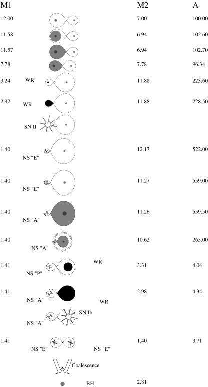
Figure 1: Evolutionary track of a massive binary star leading to the formation and coalescence of two NS.

Close NS binaries originate from two sufficiently massive main-sequence stars separated by a moderate distance of order 100 solar radii (1-st row in Fig. 1). To get a NS in the course of evolution, the mass of the progenitor star must be larger than $\approx$10M_⊙ initially or, in any case, taking into account a possible mass transfer in close binary, the mass should be $\approx$10M_⊙ during the stage of nuclear burning. The more massive the primary star is, the faster it evolves. For main-sequence stars, the time of core hydrogen burning is $t_{nucl}\propto M^{-2}$. The star burns out its hydrogen in its central parts, so that a dense central helium core with a mass $M_{He}\sim 0.1(M/M_{\odot})^{1.4}$ forms by the time when the star leaves the main-sequence. The outer shell expands and the star moves towards the red super-giant region in the Hertzsprung–Russell diagram. At some stage of its evolution the star fills out its Roche lobe [Eq. (A42)] (3-rd row in Fig. 1). The hydrogen envelope starts outflowing onto the secondary, less massive star, which still resides on the main-sequence. The primary star is being continuously stripped off of its hydrogen envelope, until a naked helium core emerges. This core can be observed as a hot compact helium star, or, for more massive stars, as a Wolf–Rayet star with intensive stellar wind (5-th row).

While the mass of the primary star reduces, the mass of the secondary star increases, since the mass transfer at this stage is thought to be quasi-conservative. For not too massive main-sequence stars, $M\mathrel{\mathchoice{\vbox{\offinterlineskip\halign{\hfil$\displaystyle#$\hfil\cr<\cr\vskip 1.5pt\cr\sim\cr}}}{\vbox{\offinterlineskip\halign{\hfil$\textstyle#$\hfil\cr<\cr\vskip 1.0pt\cr\sim\cr}}}{\vbox{\offinterlineskip\halign{\hfil$\scriptstyle#$\hfil\cr<\cr\vskip 0.5pt\cr\sim\cr}}}{\vbox{\offinterlineskip\halign{\hfil$\scriptscriptstyle#$\hfil\cr<\cr\vskip 0.5pt\cr\sim\cr}}}}20$ M_⊙, no significant stellar wind mass loss occurs which could, otherwise, remove matter from the binary. The secondary star acquires a large angular momentum due to the infalling material, so that its outer envelope can be spun up to an angular velocity close to the limiting (Kepler orbit) value. Such massive rapidly rotating stars are observed as Be-stars. During the conservative stage of mass transfer, the semi-major axis of the orbit first decreases, reaches a minimum when the masses of the binary components become equal to each other, and then increases. This behavior is dictated by the angular momentum conservation law [Eq. (A26)]. After the completion of the conservative mass transfer, the initially more massive star becomes less massive than its initially lighter companion. The parameter $q=M_{2}/M_{1}$ becomes larger than 1. In a short time, typically $\sim 10\%$ of the hydrogen burning time, the nuclear evolution of the helium star is completed and, provided its mass is larger than 2-3 $M_{\odot}$, it explodes as a core-collapse supernova type-II leaving a neutron star as its remnant.

Even for asymmetric supernova explosions, most of such binaries do not get disrupted. This is because the mass ratio $q=M_{2}/M_{1}$ of the pre-supernova binary becomes generally high, $q\approx 3$–5. After the first SN explosion, the binary system consists of a Be-star and a NS in an elliptical orbit (8-th row). Orbital evolution following the SN explosion is described in more detail in an Appendix [Eqs. (A35–A40)].

Be-stars have very rapidly rotating envelopes but in other respects they do not differ from ordinary main-sequence stars. After the completion of hydrogen burning in the core, a Be-star starts expanding until it fills out its Roche lobe while passing through the periastron of an elliptical orbit (10-th row). This initiates the second episode of the mass transfer, which takes place on the thermal scale of the Be-star, typically $\sim 10^{-6}M_{\odot}$/yr. However, this mass transfer is qualitatively different from the first one, since the mass transfer is now on to a compact star. Once the accretion rate exceeds the value which provides the luminosity equal to the Eddington luminosity limit near the NS surface ($\sim 10^{-8}M_{\odot}$/yr), the NS cannot accrete all the infalling matter. The so-called common envelope stage arises (11th row) during which the neutron star finds itself inside quite dense outer layers of the companion star. Numerical hydrodynamic calculations [67, 68] show that the dynamical friction of the orbiting NS leads to an efficient transfer of the orbital angular momentum to the common envelope, thus dispersing it on a very short timescale (typically, $10^{3}-10^{4}$ years). The semi-major axis of the binary system reduces dramatically [Eq. (A41)], which results in the formation of a close binary system consisting of a NS and a WR star (12th row). Alternatively, the NS can sink into the center of its red giant companion (the so-called Thorne–Zytkow object; not shown in this Figure).

In a short time ($\mathrel{\mathchoice{\vbox{\offinterlineskip\halign{\hfil$\displaystyle#$\hfil\cr<\cr\vskip 1.5pt\cr\sim\cr}}}{\vbox{\offinterlineskip\halign{\hfil$\textstyle#$\hfil\cr<\cr\vskip 1.0pt\cr\sim\cr}}}{\vbox{\offinterlineskip\halign{\hfil$\scriptstyle#$\hfil\cr<\cr\vskip 0.5pt\cr\sim\cr}}}{\vbox{\offinterlineskip\halign{\hfil$\scriptscriptstyle#$\hfil\cr<\cr\vskip 0.5pt\cr\sim\cr}}}}10^{5}$ years), the companion WR star explodes as a supernova type Ib, thus producing a second neutron star. During this explosion, the system is more likely to be disrupted than during the first SN explosion, since the exploding star is now more massive than its companion. Surviving systems form close high-eccentric NS binaries, similar to the NS binary PSR 1913+16. Orbital parameters of such binaries change exclusively due to the emission of gravitational waves (see section A1.4). If the neutron stars are close enough, they coalesce in a time shorter than $t_{H}$.

2.2.5 Black hole formation parameters

So far, we have considered the formation of individual NS and their binaries. It is believed that very massive stars end up their evolution with the formation of stellar mass black holes. We will discuss now the formation of an individual black hole.

In the analysis of BH formation, new important parameters appear. The first one is the threshold mass $M_{cr}$ beginning from which a main-sequence star, after the completion of its nuclear evolution, can collapse into a BH. This mass is not well known, different authors assume different values: van den Heuvel and Habets [69] — 40M_⊙; Woosley et al. [70] — 60M_⊙; Portegies Zwart, Verbunt, Ergma [71] — more than $20M_{\odot}$. A simple physical argument usually cited in the literature is that the mantle of the main-sequence star with $M>M_{cr}\approx$30M_⊙ is bound before the collapse with the binding energy well above $10^{51}$ ergs (typical supernova energy observed), so that the supernova shock is not strong enough to expel the mantle.

The second parameter is the mass $M_{BH}$ of the formed BH. There are various studies as for what the mass of the BH should be (e.g. [72, 73, 74, 75]). In some papers a typical BH mass was found to be not much higher than the upper limit for the NS mass (Oppenheimer–Volkoff limit $\sim$1.6–2.5M_⊙, depending on the unknown equation of state for the neutron star matter) even if the fallback accretion onto the supernova remnant is allowed [72]. However, observations strongly indicate much higher masses of BH candidates, of the order of 6–10M_⊙ (see Table 2). To obtain such BH masses, it is sometimes assumed [73] that $M_{cr}\sim$80M_⊙. Recently, a continuous range of BH masses up to 10-15 M_⊙ was derived in calculations [75]. Since the present day calculations are still unable to reproduce self-consistently even the supernova explosion, we have parameterized the BH mass $M_{BH}$ by the fraction of the pre-supernova mass $M_{*}$ that collapses into BH: $k_{BH}=M_{BH}/M_{*}$. In fact, the pre-supernova mass $M_{*}$ is directly related with $M_{cr}$, but the form of this relationship is somewhat different in different scenarios for massive star evolution. According to our parameterization, the minimal BH mass can be $M_{BH}^{min}=k_{BH}M_{*}$, where $M_{*}$ itself depends on $M_{cr}$. We have varied $k_{BH}$ in a wide range from 0.1 to 1.

The third parameter, similar to the case of NS formation, is a possible kick velocity ${\bf w}_{BH}$ attributed to a newly formed BH. In general, one expects that a BH should acquire a smaller kick velocity than a NS, as black holes are more massive than neutron stars. In our calculations we have adopted the relation

$$\frac{w_{BH}}{w_{NS}}=\frac{M_{*}-M_{BH}}{M_{*}-M_{OV}}=\frac{1-k_{BH}}{1-M_{OV}/M_{*}}\,,$$ (7)

where $M_{OV}=2.5$M_⊙ is the maximum NS mass. When $M_{BH}$ is close to $M_{OV}$, the ratio $w_{BH}/w_{NS}$ approaches 1, and the low-mass black holes acquire kick velocities similar to those of neutron stars. When $M_{BH}$ is significantly larger than $M_{OV}$, the parameter $k_{BH}=1$, and the BH kick velocity becomes vanishingly small . As we show below, the allowance for a quite moderate $w_{BH}$ strongly increases the coalescence rate of binary BH. A recent analysis of space velocities of some BH candidates did not reveal the need for a non-zero $w_{BH}$ [76]. However, other studies show that some kick velocity can arise during the BH formation, and its presence does not contradict the observational data [77]. From a theoretical point of view, the presence of a moderate kick velocity imparted to a BH during its formation seems very plausible [75].

2.2.6 Binary black hole merging with $w_{BH}=0$: typical example

We begin from the simplest assumption $w_{BH}=0$. The more realistic cases $w_{BH}\neq 0$ will be considered in subsection 2.3.2. In contrast to NS+NS binaries, the BH+BH and BH+NS binary systems have not been observed so far. There is no way of recovering from observations the range of progenitors for such binary systems. We can only apply the population synthesis method and derive theoretically the parameters of all the binaries, including the BH+BH and BH+NS pairs, that should be produced at the end of the evolution of very massive binary stars.

In addition to the evolutionary uncertainties existing for stars evolving to binary NS systems, new uncertainties arise for very massive stars with initial masses $M\mathrel{\hbox to0.0pt{\lower 3.0pt\hbox{$\mathchar 536\relax$}\hss}\raise 2.0pt\hbox{$\mathchar 318\relax$}}40M_{\odot}$. First of all, a large mass-loss via stellar wind is observed for such stars. According to current views, a massive single star can lose more than a half of its initial mass already on the main-sequence. Further rapid mass decrease is expected during a helium star stage. There is no general agreement as to how to describe the mass loss of a massive star. Yet, one can consider two extreme cases for the mass loss via stellar wind: a slow mass-loss and very fast one. Since the exact description of the stellar wind mass loss is not known, we have considered both options in our numerical simulations (for more details, see [63]). A typical evolutionary track that leads to the formation of coalescing binary BH system, assuming a low mass-loss scenario, is shown in Fig. 2.

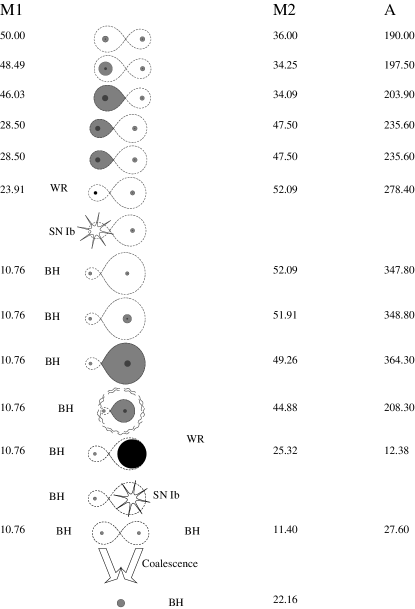
Figure 2: Evolutionary track of a massive binary star leading to the formation and coalescence of two BH. The low stellar wind mass loss scenario is used.

Before proceeding further with evolutionary calculations, we want to explain qualitatively how a merging BH binary can form even in the framework of an extremely high mass loss. The high mass loss makes the binary system wider, according to Eq. (A29), so it should have been quite tight before the phase of an active mass-loss. Consider two already existing black holes, each of 10 $M_{\odot}$, in a circular orbit. The orbital separation should be $<20R_{\odot}$ for the binary to merge within the $t_{H}$ (see Fig. 19). This means that the radius of a Wolf-Rayet (helium) star that collapsed second, in the course of a binary evolution, to form a BH should have been less than 10 $R_{\odot}$. The mass of the pre-collapse star could not be smaller than 10 $M_{\odot}$, since $k_{BH}\leq 1$. Such massive helium stars have very small radii ($\sim 1R_{\odot}$) and do not expand too much before the collapse, so the requirement $R<10R_{\odot}$ is fulfilled. The life-time of a massive helium star is about $10^{5}$ years, since it loses mass at a high rate of $10^{-5}$ $M_{\odot}$/yr. The star can lose a sizable fraction, maybe a half, of its mass before the collapse. Thus, we will be dealing with a 20 $M_{\odot}$ helium star in pair with the first 10 $M_{\odot}$ BH in a circular orbit of radius $a\approx 13R_{\odot}.$ (We applied Eq. (A29) to calculate the radius of the resulting orbit.) Note that the 8 $R_{\odot}$ Roche lobe of a 20 $M_{\odot}$ helium star is still quite large. To form such a close WR+BH binary, a common envelope stage is needed. The 20 $M_{\odot}$ He core corresponds to at least 55 $M_{\odot}$ main-sequence star, as follows from Eq. (A44). According to the models by Schaller et al. [78], a massive star loses about a half of its initial mass on the main-sequence, so to form a common envelope with 10 $M_{\odot}$ BH the star has to lose $\sim 25M_{\odot}$ while on the main-sequence. This means that the common envelope stage should have started with a 30 $M_{\odot}$ red super-giant filling its Roche lobe and having a 10 $M_{\odot}$ BH as a companion. The mass ratio in such a system is high enough for the common envelope to develop. The orbital separation at the common envelope stage should have decreased by 6-12 times, according to Eq. (A43), depending on the parameter $\alpha_{CE}$ and the exact value of the red giant mass. So, before the common envelope stage, the orbital separation should have been $\sim 130R_{\odot}$. The orbit should be somewhat smaller than this (i.e., about 120 $R_{\odot}$ or less) when the first BH forms, because of the strong wind from the red giant and loss of the total mass. And in order to collapse first, the mass of the primary star must have been at least 60 $M_{\odot}$. Assuming isotropic stellar wind and using again Eq. (A29), we conclude that the initial system could have widened at most $(60+55)/(10+30)\approx 3$ times since the time of its formation, i.e. the initial separation of the progenitor binary should be larger than 40 $R_{\odot}$. The initial separation of 50 $R_{\odot}$ is sufficient enough to harbour two 60 $M_{\odot}$ stars since their radii are less than 20 $R_{\odot}$ on the main-sequence. Even though such initially close massive binaries are rare, they should exist. Thus, we see that some fraction of massive binary stars should have ended up as sufficiently close pairs of black holes.

2.3 Effects of the kick velocity

The picture outlined above changes if a non-zero kick velocity is present in the process of formation of a NS or a BH. This, in turn, has a significant effect on the expected rate of compact binary mergings, which is of primary interest for our study. In general, the formation of a compact object (NS or BH) is accompanied, both, by a mass loss from the system and by a kick velocity. The effects of kick velocity during supernova explosions were considered in many papers (see e.g. [79, 80] and also A2). The general formulae for the condition of system’s disruption and for parameters of the resulting elliptical orbit, if the system remains bound, are derived in A2, see Eqs. (A35), (A36), (A38). Here we will present qualitative arguments enabling the reader to see the main consequences of a non-zero kick velocity. We restrict our attention to circular orbits and assume equal probabilities for all possible orientations of the kick velocity vector ${\mathbf{w}}$. We argue that a moderate (not too large) kick velocity increases the rate of binary mergings. This happens because a moderate kick velocity does not change too much the likelihood of the system’s disruption, but, at the same time, always makes the periastron of the resulting elliptical orbit smaller than it would have been without a kick. As a result, some of the binaries, whose coalescence time without a kick would be longer than the Hubble time, now get a chance to merge in a time shorter than $t_{H}$. This increases the number of detectable gravitational wave sources.

2.3.1 Effect of the kick velocity on the disruption of a binary system

The collapse of a star to a BH, or its explosion leading to the formation of a NS, are normally considered as instantaneous. This assumption is well justified in binary systems, since typical orbital velocities before the explosion do not exceed a few hundred km/s, while most of the mass is expelled with velocities about several thousand km/s. The exploding star $M_{1}$ leaves the remnant $M_{c}$, and the binary loses a portion of its mass: $\Delta M=M_{1}-M_{c}$. The relative velocity of stars before the event is

$$V_{i}=\sqrt{G(M_{1}+M_{2})/a_{i}}.$$ (8)

Right after the event, the relative velocity is

$${\mathbf{V}}_{f}={\mathbf{V}}_{i}+{\mathbf{w}}\,.$$ (9)

Depending on the direction of the kick velocity vector ${\mathbf{w}}$, the absolute value of ${\mathbf{V}}_{f}$ varies in the interval from the smallest $V_{f}=|V_{i}-w|$ to the largest $V_{f}=V_{i}+w$. The system gets disrupted if $V_{f}$ satisfies the condition (see A2):

$$V_{f}\geq V_{i}\sqrt{\frac{2}{\chi}}$$ (10)

where $\chi\equiv(M_{1}+M_{2})/(M_{c}+M_{2})$.

Let us start from the limiting case when the mass loss is practically zero ($\Delta M=0$, $\chi=1$), while a non-zero kick velocity can still be present. This is a model for a BH formation with $k_{BH}=1$. It follows from Eq. (10) that, for relatively small kicks, $w<(\sqrt{2}-1)V_{i}$, the system always (independently of the direction of ${\mathbf{w}}$) remains bound, while for $w>(\sqrt{2}+1)V_{i}$ the system always unbinds. By averaging over equally probable orientations of ${\mathbf{w}}$ with a fixed amplitude $w$, one can show that in the particular case $w=V_{i}$ the system disrupts or survives with equal probabilities. If $V_{f}<V_{i}$, the semi-major axis of the system becomes smaller than the original binary separation, $a_{f}<a_{i}$ (see Eq. (A35)). This means that the system becomes more bound than before, i.e. it has a greater negative total energy than the original binary. If $V_{i}<V_{f}<\sqrt{2}V_{i}$, the system remains bound, but $a_{f}>a_{i}$. For small and moderate kicks $w\mathrel{\mathchoice{\vbox{\offinterlineskip\halign{\hfil$\displaystyle#$\hfil\cr<\cr\vskip 1.5pt\cr\sim\cr}}}{\vbox{\offinterlineskip\halign{\hfil$\textstyle#$\hfil\cr<\cr\vskip 1.0pt\cr\sim\cr}}}{\vbox{\offinterlineskip\halign{\hfil$\scriptstyle#$\hfil\cr<\cr\vskip 0.5pt\cr\sim\cr}}}{\vbox{\offinterlineskip\halign{\hfil$\scriptscriptstyle#$\hfil\cr<\cr\vskip 0.5pt\cr\sim\cr}}}}V_{i}$, the probabilities for the system to become more or less bound are approximately equal.

In general, the binary system loses some fraction of its mass $\Delta M$. For a BH formation this corresponds to $k_{BH}<1$. In the absence of the kick velocity, the system remains bound if $\Delta M<M/2$ and gets disrupted if $\Delta M\geq M/2$ (see A2). Clearly, a properly oriented kick velocity (directed against the vector ${\mathbf{V}}_{i}$) can keep the system bound, even if it would have been disrupted without the kick. And, on the other hand, an unfortunate direction of ${\mathbf{w}}$ can disrupt the system, which otherwise would stay bound.

Consider, first, the case $\Delta M<M/2$. The parameter $\chi$ varies in the interval from 1 to 2, and the escape velocity $V_{e}$ varies in the interval from $\sqrt{2}V_{i}$ to $V_{i}$ (see A2). It follows from Eq. (A39) that the binary always remains bound if $w<V_{e}-V_{i}$, and always unbinds if $w>V_{e}+V_{i}$. This is a generalization of the formulae derived above for the limiting case $\Delta M=0$. Obviously, for a given $w$, the probability for the system to disrupt or become less bound increases when $\Delta M$ becomes larger. Now turn to the case $\Delta M>M/2$. The escape velocity of the compact star becomes $V_{e}<V_{i}$. The binary is always disrupted if the kick velocity is too large or too small: $w>V_{i}+V_{e}$ or $w<V_{i}-V_{e}$. However, for all intermediate values of $w$, the system can remain bound, and sometimes even more bound than before, if the direction of ${\mathbf{w}}$ happened to be approximately opposite to ${\mathbf{V}}_{i}$. A detailed calculation of probabilities for the binary’s survival or disruption requires integration over the kick velocity distribution function $f({\mathbf{w}})$ (see e.g. [80]).

2.3.2 Effect of the kick velocity on coalescence rate of compact binary systems

Here we consider binary systems that were not disrupted during the formation of a compact object. The parameters $a_{f}$ and $e$ of the resulting elliptical orbit are defined by Eqs. (A35), (A36). The distance of the closest approach between the stars is given by the orbit’s periastron $a_{p}=a_{f}(1-e)$. It follows from Eqs. (A35), (A36) that $a_{p}=a_{i}$ in the absence of kick velocity. The importance of the kick velocity $w\neq 0$ lies in the fact that, although the semimajor axis $a_{f}$ can increase or decrease under the action of the kick, the periastron distance always becomes smaller: $a_{p}<a_{i}$. This relationship follows from the combination of Eqs. (A35), (A36) plus the requirement that the system remains bound, i.e. the quantities participating in Eq. (A38) satisfy the opposite inequality. The decrease of the periastron distance plays an important role in the subsequent evolution of the binary, which consists now of a newly born compact star and its companion.

Consider, first, a normal star as the companion. Since the kick has diminished the periastron distance, as compared with the no-kick case, the normal star, while passing through the periastron, will fill out its Roche lobe in a shorter time, than it would do in the absence of the kick. After the tidal circularization of the orbit, a tighter binary is formed. Accordingly, the subsequent common envelope stage makes the binary tighter than it would otherwise do (see Eq. (A43)). As a result, the final binary system, consisting of two compact objects, will coalesce due to GW radiation in a shorter time (see Eq. (A22)). In other words, some of the binaries, which would be too broad to coalesce in $t_{H}$, become detectable sources of GW with the help of a moderate kick velocity. If the companion is already a compact star, the orbital evolution is driven exclusively by GW emission (Section A1.4). Unless the kick velocity is so big that it makes the semimajor axis $a_{f}$ very large, these binaries will also merge in a time interval shorter than the one following from the evolution without a kick.

These qualitative considerations explain the outcomes of numerical simulations with many trial systems. We are interested in results averaged over many systems with different input parameters. These results are presented below. As expected, a moderate kick velocity increases, on average, the rate of compact star mergings.

2.3.3 Coalescence rates of compact binaries

We can now present the results of our numerical calculations for the coalescence rate of compact binaries in a typical galaxy [81]. The total mass of a model galaxy is assumed to be $10^{11}M_{\odot}$. We adopt a constant star formation rate defined by Eq. (3). It is believed that Eq. (3) reflects well the situation in a galaxy like our own Milky Way.

Figure 3: NS+NS, BH+NS, and BH+BH merging rates in a $10^{11}$ M_⊙ galaxy as functions of the kick velocity parameter $w_{0}$ for Lyne-Lorimer kick velocity distribution (6). Star formation rate in the galaxy is assumed constant. BH formation parameters are $M_{*}=15$–50 M_⊙, $k_{BH}=0.25$.

In Fig. 3 we plot the NS+NS, BH+NS, and BH+BH merging rates as functions of the kick velocity parameter $w_{0}$ in the distribution (6). The calculations were performed for discrete values of $w_{0}$, but the resulting points are joined by smooth curves. The BH formation parameters were taken from the range $M_{*}=15-50M_{\odot}$ with $k_{BH}=0.25$. Both the high mass loss and the low mass loss stellar winds were considered. The broad range of $M_{*}$ and the uncertainty in the stellar winds have contributed to the spread of the results for BH+NS and BH+BH systems. The NS+NS systems arise from relatively low mass stars, so they are less sensitive to the uncertainty in the stellar wind. It is seen from Fig. 3 that the NS+NS rate lies in the range $\sim 3\times 10^{-4}$–$\sim 3\times 10^{-5}$ per year. The rates of BH+NS and BH+BH mergings are 10-100 times lower. For the limiting case of zero kick velocity ($w_{0}=0$) our rates agree with the independent estimates of Tutukov and Yungelson [82]. In the same limit $w_{0}=0$, our rate for NS+BH binaries ($\sim 10^{-6}$ per year) is smaller than the estimate by Bethe and Brown [73], who obtained the rate $\sim 2\times 10^{-5}$ per year. However, we believe that their estimate was derived from a somewhat simplified picture of binary evolution.

As expected, the BH+NS and BH+BH rates have a tendency to grow with the increase of kick velocity from zero. This is seen on the graph as the rise of the NS+BH and BH+BH curves for small and moderate $w_{0}$ (up to $w_{0}\sim 100$ km/s). For much larger values of $w_{0}$, the kick velocity contributes mostly to the disruption of binary systems, and this is why the curves have a tendency to turn down. Generally speaking, the NS+NS rate should also grow for small deviations of $w_{0}$ from zero. However, since the NS mass is smaller than the BH mass, the increase of the NS+NS rate takes place for only a small value of $w_{0}$, not resolvable on the graph. For larger values of $w_{0}$, the kicks mostly disrupt the binaries, and the NS+NS curve goes down. The value of $w_{0}$ preferred by the radio-pulsar observations lies in the range 200–400 km/s.

For a broad range of used parameters and despite all the remaining uncertainties, the results of evolutionary calculations show that the number of coalescing BH+BH pairs is only a factor 10-100 smaller than the number of coalescing NS+NS pairs. This relationship may have a simple explanation and can be traced back to the initial conditions of star formation. The line of argument is as follows. Let us take the NS mass at 1.4$M_{\odot}$ (a typical mass well confirmed by existing observations), and the BH mass at 8.5M_⊙ (the mean value for BH candidates from Table 2). Assume that the lower initial mass of NS progenitors is $M(NS)\approx 10$M_⊙, while the threshold for a BH formation is at the maximum of the estimates quoted above: $M(BH)>M_{cr}=80$M${}_{\odot}\,$. Applying the Salpeter initial mass function for the formation rate of stars in the Galaxy (see Eq. (2)):

$$\frac{dN}{dtdM}\simeq 1M_{\odot}(M/M_{\odot})^{-2.35}$$

and using the lower limits of integration, one finds

$$\frac{N(M>80M_{\odot})}{N(M>10M_{\odot})}=\left(\frac{80M_{\odot}}{10M_{\odot}}\right)^{-1.35}\simeq 0.06.$$

This ratio should be valid for binary stars too. It is reasonable to expect then that despite differences and complexities of binary evolution, the ratio of coalescence rates will be given, approximately, by the same number:

$$\frac{{\cal R}_{BH}}{{\cal R}_{NS}}=\left(\frac{80M_{\odot}}{10M_{\odot}}\right)^{-1.35}\simeq 0.06.$$ (11)

This expectation turns out to be in rough agreement with the results of detailed evolutionary calculations presented above.

The derived rates ${\cal R}_{G}$ for a single galaxy can be extrapolated to larger volumes. For the purposes of GW detection it is important to know the rate of events from distances accessible to the instruments in LIGO, VIRO, GEO–600. These are large distances up to and above 100 Mpc (see Section 7). In such a large volume one can regard galaxies as being distributed homogeneously, and at the same time, one can neglect effects of cosmological evolution on star formation initial conditions, etc. To derive the average density of Galactic events in a large volume one can use different approaches. One possibility is to use the luminosity of galaxies per Mpc³ (as in  [24]). Alternatively, one can rely on the estimate of density of baryons bound in stars. The baryon density $\rho_{b}$ is often expressed in terms of the dimensionless parameter $\Omega_{b}\equiv\rho_{b}/\rho_{cr}$, where $H_{0}$ is the present value of the Hubble parameter and $\rho_{cr}=3H_{0}^{2}/8\pi G$ is the critical density. Then, one can relate the Galactic rate ${\cal R}_{G}$ per a $10^{11}M_{\odot}$ galaxy with the volume rate ${\cal R}_{V}$ per 1 $\hbox{Mpc}^{3}$:

$${\cal R}_{V}=3\times 10^{-3}{\cal R}_{G}\frac{\epsilon}{(0.5)}\frac{\Omega_{b}h_{70}^{2}}{(0.0045)}\hbox{Mpc}^{-3}$$ (12)

where $\epsilon$ is the fraction of binary stars and $h_{70}=H_{0}$/(70 km/s Mpc). This estimate agrees with that of [24] assuming $\epsilon=1$ (all stars are binaries). The available astronomical measurements of the total baryon budget give $\Omega_{b}\approx 0.0015h_{70}^{-1}$ in galactic disks and $\Omega_{b}\approx 0.003h_{70}^{-1}$ in bulges of spirals and ellipticals [83] (as well as the somewhat larger values [84]). On the other hand, estimates of $\Omega_{b}$ based on the primordial nucleo-synthesis considerations give as much as $\Omega_{b}h^{2}=0.016$, but this number can also be a factor of 2 smaller [85]. Formula (12) can be rewritten as

$${\cal R}_{V}=0.1{\cal R}_{G}\frac{\epsilon}{0.5}\frac{\Omega_{b}h^{2}}{0.016}\left(\frac{r}{\hbox{Mpc}}\right)^{3}.$$ (13)

When comparing our numerical simulations, described below, with qualitative estimates, we rely on the relationship

$${\cal R}_{V}=0.1{\cal R}_{G}\left(\frac{r}{\hbox{Mpc}}\right)^{3}.$$ (14)

This result for ${\cal R}_{V}$ is based on ${\cal R}_{G}$ for spiral galaxies. For elliptical galaxies the star formation process is more like an instantaneous event rather than a continuing process described by (3). The coalescence rates have been calculated for elliptical galaxies too. However, it was shown [86] that the contribution of elliptical galaxies to the coalescence rates from the discussed distances is only about 10-20 %.

3 Detection Rates

Having found the coalescence rates ${\cal R}_{V}$ for binaries of different nature, one can now predict the detection rates of these binaries in a given GW detector. We argue that binary black holes have a better SNR than of binary neutron stars, and, despite their lower abundance, the BH+BH and BH+NS pairs should be seen more often than NS+NS pairs. In the first subsection, we derive the detection rates that are based on the ${\cal R}_{G}$ described above. In the second subsection, we discuss possible modifications to our conclusion in connection with the recently proposed scenario [87], which applies to very massive stars. Since the proposed scenario can affect only the BH+BH detection rates, we concentrate on these systems emphasizing the important role of kick velocities.

3.1 Detection rates in the usual picture

The rate of NS+NS coalescences is higher than the rate of NS+BH and BH+BH coalescences. However, the BH mass is significantly larger than the NS mass. A binary involving one or two black holes, placed at the same distance as a NS+NS binary, produces a significantly larger amplitude of gravitational waves (see Section 8 and A1). With a given sensitivity of the detector (fixed SNR), a BH+BH binary can be seen at a greater distance than a NS+NS binary. Hence, the registration volume for such bright binaries is significantly larger than the registration volume for relatively weak binaries. The detection rate of a given detector depends on the interplay between the coalescence rate (spatial density of sources) and the detector’s response to sources of one or another kind.

Coalescing binaries emit gravitational wave signals with a well known time-dependence (waveform). This allows one to use the technique of matched filtering [4]. The signal-to-noise ratio $S/N$ depends mostly on the “chirp” mass of the binary system ${\cal M}=(M_{1}+M_{2})^{-1/5}(M_{1}M_{2})^{3/5}$ and its distance $r$. The accurate formula for $S/N$ is presented in Section 8 (formula (134)). Here, we will use its simplified version which is sufficient for our purposes ([4], see also [88]):

$$\frac{S}{N}=3^{-1/2}\pi^{-2/3}\frac{G^{5/6}}{c^{3/2}}\frac{{\cal M}^{5/6}}{r}f^{-1/6}/h_{\rm rms}(f)\,.$$ (15)

At a fixed level of $S/N$, the detection volume is proportional to $r^{3}$ and therefore it is proportional to ${\cal M}^{5/2}\,$. The detection rate ${\cal D}$ for binaries of a given class is the product of their coalescence rate ${\cal R}_{V}$ with the detector’s registration volume $\propto{\cal M}^{5/2}\,$ for these binaries.

Let us start from a qualitative discussion of the expected ratio

$$\frac{{\cal D}_{BH}}{{\cal D}_{NS}}=\frac{{\cal R}_{BH}}{{\cal R}_{NS}}\left(\frac{{\cal M}_{BH}}{{\cal M}_{NS}}\right)^{5/2}\,$$ (16)

where ${\cal D}_{BH}$ and ${\cal D}_{NS}$ refer to BH+BH and NS+NS pairs, respectively. Here, we discuss the ratio of the detection rates, rather than their absolute values. The derivation of absolute values require detailed evolutionary calculations which will be discussed later. As a rough estimate for ${\cal R}_{BH}/{\cal R}_{NS}$ one can take Eq. (11). Then, Eq. (16) gives a remarkable result:

$$\frac{{\cal D}_{BH}}{{\cal D}_{NS}}=\left(\frac{80M_{\odot}}{10M_{\odot}}\right)^{-1.35}\left(\frac{8.5M_{\odot}}{1.40M_{\odot}}\right)^{5/2}\simeq 5.5\,.$$ (17)

This ratio becomes even larger than $5.5$, if one takes $M_{cr}<80M_{\odot}$ as usually assumed. Thus, the registration rate of BH mergers is expected to be higher than that of NS mergers. This estimate is, of course, very rough, but it can serve as an indication of what one can expect from detailed calculations.

In Fig. 4 we display the results of numerical calculations for the absolute registration rates of various binaries. The detector sensitivity is taken as $h_{rms}=10^{-21}$ at $f=100Hz$, as expected for initial instruments in LIGO, VIRGO, GEO600. It is assumed that $S/N=1$. Since the most interesting results refer to systems with black holes, we vary the black hole formation parameter $k_{BH}$. The calculations were performed assuming the Lyne-Lorimer kick velocity distribution with $w_{0}=400$ km/s. The vertical dispersion of the results is due to the uncertainty in the parameter $M_{cr}$.

Figure 4: The detection rate ${\cal D}$ of GW events in a detector with the sensitivity $h_{\rm rms}=10^{-21}$ at frequency 100 Hz and the signal-to-noise level $S/N=1$, as a function of BH formation parameter $k_{BH}$. The calculations were performed for the Lyne–Lorimer kick velocity distribution with $w_{0}=400$ km/s. The spread of ${\cal D}$ at fixed $k_{BH}$ is due to variation of the parameter $M_{cr}$ from 15 $M_{\odot}$ to 50 $M_{\odot}$. The bottom rectangular area is drawn for binary NS coalescences. Their rate is independent of $k_{BH}$ (as it should be) and predicts a couple of events per 1–3 years at this level. The total detection rate can be 2–3 orders of magnitude higher then the NS+NS rate at the expense of BH+BH and BH+NS coalescences. The hatched area shows the region of the most probable parameters for the low stellar wind mass loss scenario. Inside this region the outcomes of calculations are in agreement with the upper limit on the galactic number of binary BH with radiopulsars (less than 1 per 700 single pulsars) and the galactic number of BH candidates similar to Cyg X–1 (from 1 to 10).

It is seen from the graph that under the formulated conditions one can expect to see a couple of NS+NS coalescences in 1-3 years of observations, at a $S/N=1$. These systems are located, roughly, at a distance of 100 Mpc. The SNR is higher for closer systems, but the expected event rate would be lower; for more distant systems, the event rate increases, but the SNR becomes smaller than 1. So, it is unlikely that NS+NS coalescences will be detected by the initial instruments.

The situation is significantly better for systems involving black holes. As is seen from Fig. 4, the total registration rate of all binaries, including BH+BH and BH+NS pairs, can be 2–3 orders of magnitude higher than the registration rate of NS+NS systems alone, mostly at the expense of massive BH pairs. This is true unless the $k_{BH}$ parameter is very small, $k_{BH}<0.4$. The hatched area shows the results of calculations with the stellar wind parameters taken from the “most probable” region. This means that under this choice of the parameters, the outcomes of other evolutionary tracks are in agreement with observations, namely, in agreement with the upper limit on the number of binary pulsars with BH (less than 1 per 700 single radio-pulsars) and with the number of Cyg X-1-like BH candidates (from 1 to 10 per Galaxy). Inside this region, one should count on 100 registrations (at the level $S/N=1$), mostly from BH mergers. The mean total mass of the BH pairs in the hatched area is around $M=30M_{\odot}$. The simplified formula (15), used in the construction of Fig. 4, overestimates the $S/N$ for pairs heavier than $30M_{\odot}$, as shown in Section 8. However, a correction for more massive binaries is not expected to change significantly the derived total registration rate.

For a reliable detection, the $S/N$ ratio should be at least 2 in each of a network of four or more antennas. Then, the calculated detection rates should be decreased by at least a factor $(S/N)^{3}=8$. This is because of the scaling $S/N\propto 1/r$ and ${\cal D}\propto r^{3}\propto(S/N)^{-3}$. Then, the expected detection rate of merging BH+BH pairs is up to 10 events per year. As will be explained in Section8, the $S/N$ ratio is somewhat different for the three different instruments: LIGO, VIRGO and GEO. For a coalescing pair with a total mass $M=30M_{\odot}$ the SNR is roughly 4 for sources at a distance of 100 Mpc. (The performance of VIRGO is expected to be better than that of other instruments, since VIRGO will be more sensitive at lower frequencies and can track the binary for a larger number of cycles.) If one is satisfied with $S/N=2$, the accessible radius increases to $r=$ 200 Mpc. Then, the calculated detection rate (several per year) is in agreement with formula (14) if one takes for coalescing black holes a reasonable galactic rate ${\cal R}_{G}=3\times 10^{-6}$ and $r=$ 200 Mpc. In its turn, this value for ${\cal R}_{G}$ fits well the event rate derived from numerical simulations, as displayed in Fig. 3.

Thus, taking into account all the remaining uncertainties, we conclude that the initial network is likely to see each year 2-3 coalescing black hole binaries with the total mass around $30M_{\odot}$, at an SNR level of about 2–3.

3.2 Non-standard scenarios and effects of kick velocities
on BH+BH detection rate

Some of the recent evolutionary calculations [87] assume that the primary stars with initial masses $M_{1}>40M_{\odot}$ never fill their Roche lobes, so that the components of the binaries evolve like single stars. As a result, the binary BH systems would be too wide to merge in $t_{H}$. Although we think the scenario [87] will face observational difficulties, since it will lead to the too small number of binaries involving a BH and a massive blue star (Cyg X–1-like systems), we consider it necessary to follow in detail the possible fate of binary BH systems. We argue that the kick velocity accompanying the BH formation increases the eccentricity of the binary, decreases its coalescence time, and thus keeps the detection rate at almost the same level as discussed in section 3.1. In addition, the kick velocity leads to interesting modifications in the relative orientations of the black hole spins with respect to each other and with respect to the orbital angular momentum.

We have adopted the proposed scenario [87] and have carried out population synthesis calculations by varying the kick velocity parameter. The binary BH merging rate was derived for a model galaxy of $10^{11}M_{\odot}$ (assuming that all stars are formed in binaries) with a constant star formation rate. For simplicity, the kick velocity distribution was taken as a delta-function. The more complicated distributions do not change the results significantly and are not commented upon here. The results of these calculations are shown in Fig. 5. The left panel shows the merging rate, while the right panel shows the detection rate. The detection rate of binary BH coalescences is given for initial laser interferometers ($h_{\rm rms}=10^{-21}$ at $f=100$ Hz) as a function of BH kick velocity. It is seen from the plot that the merging rate and the detection rates increase rapidly with the kick. The merging and detection rates reach the maxima ${\cal R}\sim 2.5\times 10^{-5}$ yr^-1 and ${\cal D}\sim 20$ detections per year for $w\simeq 120$ km/s. Since ${\cal D}\sim{\cal M}^{5/2}{\cal R}$, the ${\cal R}(w)$ and ${\cal D}(w)$ functions have similar shapes.

Figure 5: New scenario — superhigh wind. Left: BH+BH merging rate calculated for a $10^{11}M_{\odot}$ galaxy with a constant star formation rate, as a function of the kick velocity during BH formation with $M_{cr}=35M_{\odot}$, for $k_{BH}=0.5$ and $0.75$. Right: Detection rate of BH+BH mergings by the initial laser interferometers ($h_{\rm rms}=10^{-21}$ at $f=100$ Hz), as a function of the kick velocity during BH formation.

Obviously, the kick velocity imparted to newly born black holes makes the orbits of survived systems highly eccentric. It is important to stress that some fraction of binary BH retain their large eccentricities up to the late stages of their coalescence. This signature should be reflected in their emitted waveforms and should be modeled in templates.

The asymmetric explosions accompanied by a kick velocity change the space orientation of the orbital angular momentum. On the other hand, the star’s spin axis remains fixed (unless the kick was non-central). As a result, some distribution of the angle between the BH spins and the orbital angular momentum (denoted by $J$) will be established [89]. It is interesting that even for small kicks of a few tens of km/s an appreciable fraction (30–50%) of the merging binary BH should have $\cos J<0$. This means that in these binaries the orbital angular momentum vector is oriented almost oppositely to the black hole spins. This is one more signature of imparted kicks that can be tested observationally. These effects are also discussed in a recent paper [90].

Thus, to conclude this analysis, we stress again that binary black hole coalescences remain the most likely sources to be detected first by the initial network of laser interferometers.

4 Transients and Continuous Gravitational Waves

In this Section we will discuss two distinct types of signals: (1) transient events, that last few to several milliseconds, which, on astronomical grounds, are expected to occur but emit waves of unknown phase evolution as in the case of supernovae and (2) continuous radiation, that last for several days or longer, from either newly born neutron stars or old recycled neutron stars. The strengths, duration and shapes of these signals is rather speculative and highly uncertain. On general physical grounds we should expect such sources to exist and every effort should be made in searching for these sources by taking the best advantage of current knowledge. However, since the astrophysical uncertainties are so large, we shall keep the discussion of this topic quite qualitative.

4.1 Transients

4.1.1 Supernovae and asymmetric explosions

Supernovae (of type II) are associated with violent mass ejection with velocities of order $0.001c$ and the formation of a compact remnant — a neutron star or black hole. The event has at its disposal the difference in the gravitational binding energy of the pre-collapse star and the newly formed compact star which, neglecting the former, is:

$$|E|\sim 3\times 10^{53}\left(\frac{M}{M_{\odot}}\right)^{2}\left(\frac{R}{10~{}{\rm km}}\right)^{-1}~{}\rm erg.$$ (18)

99% of this energy is carried away by neutrinos, about 1% is transferred as kinetic energy of ejecta, a fraction $10^{-4}$ of the total energy is emitted in the form of electromagnetic radiation. Depending on how asymmetric the collapse is, some fraction of the total energy should be deposited into gravitational waves; spherically symmetric collapse, of course, cannot emit any radiation. According to numerical simulations (see [91] for a review) one might expect up to $10^{-7}$ of the total energy to be emitted in gravitational waves. Together with uncertainties in the event rate, this is not a very encouraging prognosis for the initial instruments [4, 5]. It appears that a star collapsing to form a black hole is also not particularly well suited for detection by the existing resonant detectors and forthcoming interferometers [92]. However, second generation interferometers should be able to see a supernova event as far as the Virgo super-cluster which contains about 200 bright galaxies and at least twice as many faint galaxies. In addition, there are a few other smaller clusters within that distance as also a large number of field galaxies. Therefore, the supernova event rate for these instruments could be as large as tens per year. Such observations would undoubtedly be of great interest and would shed light on hitherto un-understood processes that occur when a star collapses to form a compact object.

An asymmetric collapse generates gravitational waves but is not necessarily accompanied by a change of linear momentum of the exploding star. However, as we emphasized above, the observations of single and binary radio-pulsars require the presence of a significant kick velocity imparted to a newly born neutron star. The kick velocity can be as large as 200–400 km/s. This testifies for a non-axisymmetric explosion leading to an additional linear momentum acquired by the neutron star. A possible reason for this asymmetry can be related with the asymmetry of the neutrino emission during the collapse [93]. Using the observed kick velocities one can evaluate asymmetry of the explosion and calculate the amplitude of emitted gravitational waves. Nazin and Postnov [94] estimate that the mean energy carried away by the gravitational wave burst can reach the value $E_{GW}=5\times 10^{-6}M_{\odot}c^{2}$. It is interesting to note that the radiated signal belongs to the category of bursts “with memory” [95, 96]. However, the estimated strength of the asymmetric explosions is still too low to count on them as reliable sources for first detection.

4.1.2 Bar-mode and convective instabilities

Some amount of gravitational waves may be emitted during two special stages of the collapse: (1) rotation-induced bars and (2) convective instabilities set up in the core of the newly born neutron star.

If the core’s rotation is high enough it may cause the core to flatten before it reaches nuclear density, leading to an instability that transforms the flattened core into a bar-like configuration which spins about its transverse axis. Some of these instabilities could also fragment the core into two or more pieces which then rotate about each other. Both are efficient ways of losing energy in the form of gravitational waves. It is estimated [97] that the waves could carry up to $10^{-3}M_{\odot}c^{2}$ in a few ms. LIGO and VIRGO detectors can see such an event at a distance up to 50 Mpc, or about 5–10 Mpc if the waves come off at 1 kHz. GEO will also be able to see these events provided the signal comes off around 200 Hz [98].

Convective instabilities in the core of a newly born neutron star, which last for about a second after the collapse, are likely to produce gravitational radiation due to anisotropic mass distribution and motion [99]. Müller and Janka [100] find that the gravitational wave amplitude of a source at 100 kpc is $h\sim 10^{-23}$ and that the waves would come off at about 100 Hz. Since there would be about 100 cycles, one can enhance the amplitude to about $10^{-22}$ provided we know the development of the signal but this is still far too weak to be detected beyond about 10 kpc with high confidence.

4.1.3 Merger waves

The physics of the merger phase that follows the adiabatic inspiral regime of a compact binary coalescence is not known. Presently, it is a subject of active research and contains a lot of uncertainties. Some authors expect that this phase could result in detectable amounts of radiation [88] while others conclude that the merger phase is just a continuation of the inspiral phase adding on the order of 1 more cycle to the inspiral [101]. There is a lot of effort to solve this important problem by using semi-analytical and numerical techniques. It is likely that a solution will be in place by the time the first detectors will begin to operate. The fact that the coalescence waves will be preceded by inspiral waves makes the search easier, though it is not inconceivable that while the former may be observable with the aid of accurate search templates, the latter may not be. Flanagan & Hughes [88] estimate that for binary systems of total mass in excess of 25M_⊙, coalescence waves are likely to be significantly stronger than the inspiral waves. The span of a detector is larger for heavier binaries and therefore, these authors conclude, it is likely that the first gravitational wave events will be the merger phases of massive binaries.

4.1.4 Sub-stellar mass black hole binaries

The results of recent micro-lensing experiments [102] have revealed massive compact halo objects (MACHOs) of mass $0.5^{+0.3}_{-0.2}\,$M${}_{\odot}.$ Nakamura et al., [103] argue that if MACHOs are black holes then they must have formed in the early Universe and they estimate that our Galaxy may contain about $10^{8}$ black hole binaries with inspiral time scales less than the Hubble time. If this is the case then the rate of MACHO coalescences in our Galaxy is $\sim 5\times 10^{-2}$ yr${}^{-1},$ implying an event rate of few per year within 15 Mpc. As we shall see in the Data Analysis Sections, first generation interferometers should be able to detect the final inspiral phase of these systems.

4.1.5 Quasi-normal modes

A compact binary coalescing as a result of gravitational radiation reaction would most likely result in the formation of a single black hole. The newly formed hole will initially be somewhat non-spherical, and this dynamical non-sphericity will be radiated away in the form of gravitational waves. The late time behaviour of this radiation is well studied in the black hole literature and there are detailed calculations of the (quasi) normal modes for both static, i.e. Schwarzschild, and stationary, i.e. Kerr, black holes. In all cases the time-evolution of the emitted radiation is well-modeled by a quasi-periodic signal of the form

$$h(t;\tau,\omega)=Ae^{-t/\tau}\cos(\omega t)$$ (19)

where $\tau$ is the decay time-scale of the mode in question and $\omega$ is the angular frequency of the mode, both of which depend on the black hole mass and angular momentum. In all but the extreme Kerr black holes (extreme Kerr black holes are those that are spinning at the maximum possible rate) the only dominant mode, i.e. the mode for which the decay time is the longest and the amplitude is the highest, is the fundamental mode whose frequency is related to the mass $M$ and spin $a$ of the black hole via $\omega=[1-0.63(1-a)^{0.3}]/M$ where $M$ is the mass of the black hole in units $G=c=1$ and $a=J/M$ is the spin angular momentum of the hole in units of black hole mass. The decay time $\tau$ is given by $\tau=4/[\omega(1-a)^{0.45}].$ (See Ref. [104] and references therein for details.)

It is estimated [88] that during the quasi-normal mode ringing of a black hole the energy emitted might be as large as 3% of the system’s total mass. By matched filtering (cf. Sec. 8.1) it should be possible to detect quasi-normal modes, in initial interferometers, from black holes of mass in the range 60–$10^{3}$M_⊙ and at a distance of 200 Mpc. Binary black hole mergers should result in the emission of such a ring down signal during the late stages. Thus, inspiral signals emitted before the merger might aid in identifying the quasi-normal modes.

4.2 Continuous waves

Our Galaxy is expected to have at least $10^{8}$ spinning neutron stars that form roughly at a rate of one every 30 years. Some population of neutron stars is in binaries. There are a number of ways in which a single spinning neutron star could radiate away gravitational waves (if the neutron star is axisymmetric, of course, then there will be no gravitational wave emission): (1) Neutron stars normally spin at high rates (several to 500 Hz) and this must induce some equatorial bulge and flattening of the poles. The presence of a magnetic field may cause the star to spin about an axis that is different from the symmetry axis leading to a time-varying quadrupole moment. (2) The star may have some density inhomogeneities in the core/crust set up during its formation and/or subsequent convectively unstable motions of the core. (3) The presence of an accretion disc, with its angular momentum not necessarily aligned with that of the neutron star, can potentially alter axisymmetry. That and electromagnetic radiation reaction torques can induce and sustain wobble. (4) The normal modes of the neutron star fluid (radial and other oscillations) can extract rotational energy and re-emit in the form of gravitational waves. (5) There are certain classical and relativistic instabilities in the neutron star fluid which may cause the star to radiate away energy in the form of gravitational radiation. In what follows we will only discuss a sample of recent work on the radiation from spinning neutron stars.

GW amplitude from spinning asymmetric neutron stars

If $I_{zz}$ is the moment of inertia about the spin axis of a neutron star emitting gravitational waves at a frequency $f$ then the gravitational amplitude at a distance $r$ is:

$$h=3\times 10^{-27}\left(\frac{10~{}{\rm kpc}}{r}\right)\left(\frac{I_{zz}}{10^{45}~{}g~{}cm^{2}}\right)\left(\frac{f}{200~{}{\rm Hz}}\right)^{2}\left(\frac{\epsilon}{10^{-6}}\right),$$ (20)

where $\epsilon$ is the ellipticity of the star. In a simple model of an equatorial plane of elliptical cross section of semi-major axis $a_{1}$ and semi-minor axis $a_{2},$ the ellipticity is $\epsilon\equiv 1-a_{2}/a_{1}$. The ellipticity is an unknown but one can obtain an upper limit on it by attributing the observed spin-down of pulsars $\dot{P}$ to gravitational radiation back reaction, namely that the change in the rotational energy $E=I\Omega^{2}/2$ is equal to gravitational wave luminosity. Then, the ellipticity is related to the spin-down rate of a pulsar via

$$\epsilon=5.7\times 10^{-6}\left(\frac{P}{10^{-2}~{}{\rm s}}\right)^{3/2}\left(\frac{\dot{P}}{10^{-15}}\right)^{1/2}.$$ (21)

Since one knows the observed values of $P$ and $\dot{P}$ one can obtain an upper limit on $\epsilon$ using the above equation. Following this method one can find that for the Crab pulsar $\epsilon\leq 7\times 10^{-4}$ and the gravitational amplitude is $h\leq 10^{-24}.$ One concludes that Crab will have a sufficiently large amplitude to be observable with the aid of GEO detector [6] in 1 year of continuous observing, if all of its spin down can be attributed to the emission of GW. It is unlikely that the ellipticity is so large. Yet, the prospect of seeing Crab event at a 10th or a hundredth of this ellipticity is quite good with first/second generation of interferometers.

In the next two paragraphs we will discuss some new developments in relativistic astrophysics that could lead to potential GW sources.

Relativistic instabilities in young neutrons stars

Chandrasekhar [105] and Friedman & Schutz [106] discovered an instability (now called the CFS instability) in the fundamental, or “f”, mode of a neutron star fluid, arising as a result of GW emission. The mode goes unstable above a critical spin frequency of the star and progressively grows, instead of decaying, by emitting gravitational waves.

The physics behind this instability can be understood in the following manner: Imagine exciting a mass-quadrupole mode – that is a non-uniform distribution of mass – in a non-spinning star. The mass inhomogeneity will travel on the surface of the star and this dynamical asymmetry will cause the star to radiate gravitational waves. After a while, all the energy in the mode will be radiated away and the mode will decay. Now consider a spinning neutron star in which a co-rotating and counter-rotating modes are excited. These fluid modes have a certain pattern speed on the surface of the star. For low spin rates both these modes will decay in course of time by emitting gravitational waves. But as the neutron star is spun up above a critical rate, to an external inertial observer both modes will appear to be traveling in the same sense as the rotation of the star. Therefore, the mode counter-rotating relative to the star will emit positive angular momentum, causing the angular momentum associated with the mode to enhance, or for the amplitude of the mode to increase. In other words, a mode counter-rotating relative to the star, but seen co-rotating relative to the inertial observer, can only emit negative angular momentum which causes its own angular momentum to increase. The energy for this enhancement is supplied by the spin angular momentum of the neutron star. Thus, while the mode co-rotating with the star’s spin will decay, the mode counter-rotating with the spin will grow in amplitude and emit more and more radiation. This will go on until the mode has sucked out enough angular momentum of the star to make the counter-rotating mode appear to be counter-rotating with respect to an inertial observer too.

It is suspected that the CFS instability will not work in the presence of viscosity and hence it may be unimportant in old neutron stars. However, newly born neutron stars will be very hot and viscous forces may be insignificant in them. Recently, Andersson [107] discovered another class of modes called $r$–modes, which — unlike CFS modes that are mass-quadrupole moments — are current-quadrupole moments, that are unstable at all spin frequencies. The role of these modes may be significant in young neutron stars. It is proposed that $r$–modes are responsible for the limit on the spin frequencies of newly born neutron stars [108]. Owen et al. [109] have computed the efficiency with which these modes extract energy out of the system and the expected gravitational wave amplitude from isolated neutron stars, as well as from the ensemble of all sources up to cosmological distances. They conclude that the second generation of interferometric antennas will be able to distinguish such a background by coincident observations with a nearby bar detector. Such observations should provide independent knowledge of the distribution of galaxies in the high-red shift Universe as also on the star formation history via the observation of $r$–modes associated with the formation of neutron stars and pulsars.

Neutron stars in X-ray binaries

In the recent years, Rossi satellite observations of the X-ray emitting binaries have shown high-frequency quasi-periodic oscillations (QPO) in their X-ray power spectra. Some authors believe that these QPO could be a result of beating of two frequencies one of which is that of the neutron star. The neutron star spins inferred in this way seem to lie in a narrow range of 250–350 Hz and are all within 20 % of 300 Hz. A neutron star may be born with a high spin rate (several 100 Hz) but quickly spins down to moderate rates (several 10 Hz). In a binary system, when the companion becomes a red giant the neutron star starts accreting mass and angular momentum. Though the mass accretion rate is very low ($\dot{M}\sim 10^{-10}$ M_⊙ yr^-1) the accretion of angular momentum can spin up a neutron star and heat its crust substantially. Indeed, the millisecond pulsars are believed to be old pulsars in binaries recycled in this way. It is puzzling as to why the spin frequencies of neutron stars in X-ray binaries are all in a narrow range. Bildsten suggests [110] that absence of efficient heat transport processes make it possible to set up temperature gradients in accreting neutron stars. Provided that the temperature distribution has large scale asymmetry then the temperature sensitive electron captures in the deep crust can build up the mass quadrupole ($\sim 10^{-7}MR^{2}$) needed to radiate away accreted angular momentum and limit the spin frequency. This mechanism is present only during accretion and decreases rapidly once the accretion halts. The frequency of GW radiation will be known in advance since one knows the spin frequency of the pulsar via X-ray observations. It is argued [110] that the gravitational wave strength will be $h\sim(0.5$–$3)\times 10^{-26}$ for many of these sources and that the LIGO/VIRGO and signal recycled GEO600, can detect the strongest of these sources, Sco X-1, at an SNR of 5 with a few years of integration.

5 Astrophysical stochastic backgrounds of gravitational waves

Coalescing binaries of compact stars are at the center of our attention. A gravitational wave signal will be monitored by a detector as long as the changing frequency of the source sweeps through the detector’s window of sensitivity. The detection of a useful gravitational wave source is limited by the instrumental noise and by a possible gravitational wave noise produced by other sources. If a large population of astrophysical sources emit overlapping gravitational waves, the resulting signal will be perceived by the detector as a gravitational wave noise. In principle, this noise could be larger than the instrumental noise. The astrophysical backgrounds of gravitational waves are important in their own right, but we are discussing them mostly as possible noises preventing the detection of a signal of a greater scientific importance. The aim of our discussion is the derivation of the gravitational mean square amplitude in a given frequency interval $\Delta f$ and comparison of this number with the instrumental noise in the same interval. If the background is below the instrumental noise, it will not prevent the detection of the useful signal. In subsection 5.1 we derive general formulas for the performance of a large number of unresolved sources. In subsection 5.1.1 we discuss the population of rotating neutron stars in our Galaxy. They could constitute a major danger for the ground-based interferometers. The analysis shows that the danger arises only under quite unrealistic assumptions about the parameters of this population. In subsection 5.1.2 we discuss the stochastic gravitational wave background produced by binary white dwarfs in the Galaxy. This background dominates the LISA instrumental noise from $\sim 10^{-4}$ Hz up to $\sim 10^{-3}$ Hz, but leaves the gravitational wave sky transparent at lower and higher frequencies. Finally, subsection 5.2 comments on astrophysical backgrounds of extra-Galactic origin. Generically, these backgrounds are one order of magnitude lower than those produced by the Galactic sources.

5.1 Unresolved sources in our Galaxy

A large collection of independent sources produces signals whose intensities add. Consider $N$ identical sources located at approximately the same distance $r$ from the observer. The resulting gravitational wave field is characterized by the r.m.s. amplitude $h_{N}$:

$$h_{N}=h_{1}\sqrt{N},$$ (22)

where $h_{1}$ is the averaged amplitude of a single source. We are interested in the narrow frequency interval from $f$ to $f+\Delta f$. The radiating sources gradually change their frequency and pass through the window of interest. The crossing of the window can occur either on the way from lower to higher frequencies, as in the case of binaries, or in the opposite direction, as in the case of rotating neutron stars. To find $h_{N}$ we need to know the number $N(f,\Delta f)$ of the radiating systems in the discussed frequency interval. Denote by ${\cal R}$ the rate at which the sources appear in the window. A source is present in the window during the time $\Delta t$, where $\Delta t=\Delta f/{\dot{f}}$. Thus,

$$N(f,\Delta f)={\cal R}\Delta t={\cal R}\frac{\Delta f}{\dot{f}},$$ (23)

and

$$h_{N}=h_{1}\sqrt{{\cal R}\frac{\Delta f}{\dot{f}}}.$$ (24)

If the frequency evolution is driven by gravitational waves only, the quantity $\dot{f}$ is determined by the gravitational radiation damping. For example, in the case of a binary system, the $\dot{f}$ is given by Eq. (A19). Alternatively, the quantity $\dot{f}$ can be determined by the electromagnetic radiation damping. This takes place in the case of highly magnetized rotating neutron stars whose $\dot{f}$ is determined by electromagnetic, rather than gravitational, losses. The appearance rate ${\cal R}$ of sources of a given population in the discussed window $\Delta f$ is equal to the birthrate or to the coalescence rate of the sources as such (see, for example, ${\cal R}_{\rm coales}$ in Sec. 4). This is true as long as the number of sources remains constant during the frequency evolution throughout the window, what we always assume.

For sources driven by gravitational radiation only, formula (24) can be expressed in terms of the energy of a single radiating system and the rate ${\cal R}$. One needs to use Eq. (A16) in order to express $h_{1}^{2}$ in terms of $dE/dt$, and to take into account the relationship $dE/dt=(dE/df){\dot{f}}$. Then, Eq. (24) takes the form

$$h_{N}^{2}=\frac{G}{c^{3}}\frac{{\cal R}}{r^{2}(\pi f)^{2}}\frac{dE}{df}\Delta f.$$ (25)

Usually, the energy of the radiating system is a power-law function of the frequency $f$: $E(f)\sim f^{\alpha}$. For example, in the case of a binary star in circular orbit one derives from Eq. (A6):

$$E(f)=\frac{G^{2/3}}{2}{\cal M}^{5/3}(\pi f)^{2/3},$$ (26)

where ${\cal M}$ is the chirp mass. So, in the case of binaries, $\alpha=2/3$. For a non-axisymmetric rotating star $E(f)\sim f^{2}$, so that $\alpha=2$. Thus, Eq. (25) takes the universal form

$$h_{N}^{2}=\frac{G}{c^{3}}\frac{{\cal R}}{r^{2}(\pi f)^{2}}\alpha E(f)\frac{\Delta f}{f}.$$ (27)

The quantity $h_{N}^{2}/\Delta f$ is the mean square noise amplitude $h_{f}^{2}$ (with dimensionality Hz^-1) which participates in the expression

$$\langle h^{2}\rangle=\int\limits_{f_{\min}}^{f_{\max}}h_{f}^{2}df\,,$$ (28)

and can now be compared with the frequency-dependent instrumental noise. We will work with the dimensionless spectral amplitude

$$h_{N}(f)\equiv h_{N}\sqrt{\frac{f}{\Delta f}}=\frac{1}{r}\sqrt{\frac{G\alpha E(f){\cal R}}{c^{3}(\pi f)^{2}}}.$$ (29)

Obviously, the independent sources in a frequency bin $\Delta f$ form a kind of stochastic background if the number $N(f,\Delta f)$ is much larger than 1. A source becomes resolvable, if this number is of order 1. For a collection of evolving sources one can find the limiting frequency $f_{\lim}$ at which this happens. For fixed $\Delta f$ and ${\cal R}$, one uses the concrete function ${\dot{f}}(f)$ (arising due to the gravitational reaction force or by some other reasons) and finds $f_{\lim}$ from the requirement

$${\cal R}\frac{\Delta f}{\dot{f}}=1.$$ (30)

For a collection of binary stars one uses Eq. (A19) and finds

$$\hbox{}\,\vbox{\openup 3.0pt\halign{\strut$\displaystyle{#}$\hfil&$\displaystyle{{}#}$\hfil\cr f_{\lim}\approx&(1.2\times 10^{-3}\hbox{Hz}){\cal R}_{300}^{3/11}\left(\frac{\Delta f}{3\times 10^{-8}\hbox{Hz}}\right)^{3/11}\left(\frac{{\cal M}}{0.52M_{\odot}}\right)^{-5/11}\cr}}\,\,.$$ (31)

The appearance (coalescence) rate ${\cal R}_{300}$ is chosen for compact white dwarfs, which are expected to coalesce in our Galaxy once per 300 years. The chirp mass is normalized to 0.52 M_⊙ which is true for two CO white dwarfs with masses 0.6 M_⊙. This estimate will be needed in subsection 5.1.2 which discusses the LISA noise.

5.1.1 Noise from old neutron stars at frequencies of ground-based interferometers

Rotating neutron stars as sources of gravitational radiation can be roughly divided into two populations: One consists of old neutron stars with relatively weak magnetic fields and small electromagnetic losses. Their rotational frequency slowly decreases due to gravitational wave damping. Another population consists of young highly magnetized neutron stars. Their rotational frequency decreases much faster due to electromagnetic damping. In course of their frequency evolution, members of both populations cross the window of sensitivity of ground-based interferometers, descending from $10^{3}$ Hz to $10$ Hz. The number of sources simultaneously radiating in a given frequency interval is proportional to the birthrate ${\cal R}$ of the population and inversely proportional to the velocity of the population flow $\dot{f}$ through the window. We start from old neutron stars and then discuss young neutron stars.

The frequency evolution of old, rotating, deformed neutron stars is governed by gravitational radiation damping. Formula for $\dot{f}$, analogous to Eq. (A19) for double stars, is

$$\dot{f}=\frac{32\pi^{4}G}{c^{5}}I\epsilon^{2}f^{5},$$ (32)

where $I$ is the relevant moment of inertia and $\epsilon$ is the ellipticity (deformation) parameter. The birthrate ${\cal R}$ of neutron stars in this population can be estimated using the observed fraction of millisecond pulsars (which are thought to be old neutron stars with low magnetic fields that have been spun up by accretion in a binary system) among radio pulsars: $N_{ms}/N_{PSR}\approx 20/2000=1/100$. Remembering that the life-time of a millisecond pulsar is $t_{ms}=10^{8}$ yr and that the life-time of an ordinary radio pulsar is $t_{PSR}=10^{6}$ yr, and adopting the Galactic birth rate of radio pulsars 1 per 30 years, as for the core collapse supernovae, one can estimate the birth rate of millisecond pulsars:

$${\cal R}_{ms}={\cal R}_{PSR}\frac{N_{ms}}{N_{PSR}}\frac{t_{PSR}}{t_{ms}}\approx 3\times 10^{-6}\hbox{yr}^{-1}$$

This estimate is in agreement with the one derived in Ref. [111] from the observed space density of millisecond pulsars.

From Eq. (30) one finds the limiting frequency

$$f_{\lim}\approx 53~{}\hbox{Hz}\,\left(\frac{{\cal R}}{3\times 10^{5}\,\hbox{yr}}\right)^{1/5}\left(\frac{\Delta f}{3\times 10^{-8}\hbox{Hz}}\right)\left(\frac{I}{10^{45}\hbox{g~{}cm}^{2}}\right)^{-1/5}\left(\frac{\epsilon}{10^{-9}}\right)^{-2/5}.$$ (33)

Thus, at frequencies below $53$ Hz the population of old neutron stars is likely to produce a stochastic background. Taking $E(f)=\pi^{2}If^{2}/2$ one derives from Eq. (29):

$$h_{N}(f)=\frac{1}{r}\sqrt{\frac{G}{c^{3}}I{\cal R}}\,\approx 2\times 10^{-26}\left(\frac{10\hbox{kpc}}{r}\right)\left(\frac{{\cal R}}{3\times 10^{5}\,\hbox{yr}}\right)^{1/2}\left(\frac{I}{10^{45}\hbox{g~{}cm}^{2}}\right)^{1/2}.$$ (34)

It is interesting that this quantity does not depend on the deformation parameter $\epsilon$, as soon as $\epsilon\neq 0$. The $h_{1}^{2}$ and $\dot{f}$ are both proportional to $\epsilon^{2}$, so that $\epsilon^{2}$ cancels out in the expression for $h_{N}^{2}$. The quantity $h_{N}(f)$ is also independent of frequency $f$. The numerical level of $h_{N}(f)$ is much lower than the instrumental noise of initial and advanced ground-based interferometers. The $h_{N}(f)$ can be increased by two orders of magnitude, and hence the gravitational wave noise from old neutron stars becomes marginally detectable, only under the condition that one postulates a significantly larger (and, we believe, unrealistic) birthrate ${\cal R}$ for old neutron stars (compare with [112]).

At frequencies higher than the limiting frequency (33), the sources are resolvable during a 1 year interval of observations. However, to monitor a single neutron star one needs to know its exact location on the sky and to take care of the Doppler frequency modulation due to the Earth’s motion around Sun.

The young neutron stars differ from old neutron stars in that their electromagnetic energy loss

$${\dot{E}}_{em}=\frac{2\pi^{4}}{3c^{3}}\mu^{2}f^{4},$$ (35)

where $\mu$ is the NS magnetic moment, is significantly larger than the gravitational wave loss

$${\dot{E}}_{gw}=\frac{32\pi^{6}G}{c^{5}}I^{2}\epsilon^{2}f^{6}.$$ (36)

The ratio $x={\dot{E}}_{em}/{\dot{E}}_{gw}$ is

$$x\approx 4\times 10^{3}(\mu_{30})^{2}(\epsilon_{-6})^{-2}(I_{45})^{-2}\left(\frac{100\hbox{Hz}}{f}\right)^{2},$$ (37)

where $\mu_{30}=\mu/(10^{30}\,\hbox{G cm}^{3})$, $\epsilon_{-6}=\epsilon/10^{-6}$ and $I_{45}=I/10^{45}$ g cm². For typical parameters of young neutron stars one has $x\gg 1$. The ratio $x$ becomes comparable with 1 only for relatively weak magnetic fields, such that the magnetic moment $\mu$ satisfies the condition $\mu<1.5\times 10^{26}(\hbox{G cm}^{3})\epsilon_{-6}(f/100\,\hbox{Hz}).$ The frequency change $\dot{f}$ is determined by the electromagnetic loss and reads

$${\dot{f}}=\frac{2\pi^{2}}{3c^{3}}\frac{\mu^{2}f^{3}}{I}.$$ (38)

For $f_{lim}$ one derives

$$f_{\lim}=0.5~{}\hbox{Hz}~{}({\cal R}_{30})^{1/3}\left(\frac{\Delta f}{3\times 10^{-8}\hbox{Hz}}\right)^{1/3}(\mu_{30})^{-2/3}(I_{45})^{1/3}.$$ (39)

The averaged amplitude $h_{1}$ of a single neutron star amounts to

$$h_{1}=\frac{G\pi^{2}\sqrt{32}}{c^{4}}\frac{1}{r}If^{2}\epsilon.$$ (40)

Then, the $h_{N}(f)$ found from Eq. (24) with the help of Eq. (38) becomes

$$h_{N}(f)=\frac{4\sqrt{3}\pi G}{c^{5/2}}\frac{1}{r}I^{3/2}{\cal R}^{1/2}\epsilon\mu^{-1}f\approx 3\times 10^{-26}\left(\frac{10\hbox{kpc}}{r}\right){\cal R}_{30}^{1/2}I^{3/2}_{45}\epsilon_{-6}\mu_{30}^{-1}{f/100Hz}.$$ (41)

Thus, the gravitational wave noise from young neutron stars is at the same numerical level as the noise from old neutron stars. The appearance rate of young neutron stars is much higher than that of old neutron stars, but they flow through the window of sensitivity much faster, so that there aren’t a sufficiently large number of sources to produce a background of a high enough level. We conclude, that the populations of neither the old nor new neutron stars do present any danger for the sensitivity curves of initial and advanced ground-based instruments. It is important that the calculated noise level is below the expected level of the relic gravitational waves (see Section 6).

5.1.2 Noise from Galactic binary white dwarfs in LISA

The LISA frequency range, $10^{-4}$–$10^{-1}$ Hz, can be contaminated by the gravitational wave noise from coalescing binary white dwarfs (WD) and binary neutron stars (NS). The appearance rates ${\cal R}$ of the two populations in the sensitivity window are numerically equal to their coalescence rates. The binary WD systems are much more numerous than the binary NS systems, and the coalescence rate of the former population is significantly higher than that of the latter. The binary WD coalescence rate is about 1 per 300 yrs, while the coalescence rate of binary NS is about 1 per several 10000 years. At the same time, the chirp masses, ${\cal M}\approx 0.52M_{\odot}$ for a WD binary and ${\cal M}\approx 1.22M_{\odot}$ for a NS binary, are not so significantly different. This is why the WD background is more important than the NS background, and we consider only the former.

For a collection of sources consisting of binary stars, one can use Eqs. (A13), (A19) in Eq. (24), or, alternatively, Eq. (26) and $\alpha=2/3$ in Eq. (27). By either way one obtains

 

$${h_{N}(f)}$$

  (42)

Roughly, this is a result of performance of $\approx 10^{6}$ binaries in the frequency bin $\Delta f=f=10^{-3}$ Hz with the averaged amplitude (see Eq. (A13))

$$h_{1}=\frac{\sqrt{32}\pi^{2}G^{5/3}}{\sqrt{5}c^{4}}\frac{1}{r}{\cal M}^{5/3}f^{2/3}=2.5\times 10^{-23}\left(\frac{10\hbox{kpc}}{r}\right)\left(\frac{{\cal M}}{0.52~{}M_{\odot}}\right)^{5/3}\left(\frac{f}{10^{-3}\hbox{Hz}}\right)^{2/3}.$$ (43)

It is necessary to note that Eq.(42) gives the estimate for the amplitude averaged over the whole sky, while the real background is strongly concentrated toward the Galactic plane [36]. The response of a space-based interferometer should be modulated while the instrument is turning in its orbit. In principle, this distinctive feature of the Galactic background can be used in order to distinguish it from the backgrounds of cosmological origin [113].

In formula (42), the quantity ${\cal R}$ replaces all the astrophysical uncertainties in the binary WD evolution. At frequencies higher than $3\times 10^{-4}$ Hz the evolution of the vast majority of binary white dwarfs is totally controlled by GW emission. So, at frequencies of interest, the GW noise is fully determined by the Galactic rate of binary WD mergers and is independent of complicated details of binary evolution at lower frequencies. (For examples of calculated spectra at all frequencies see [114, 33, 34, 115].) The coalescence rate of close binary WD is known only up to a factor of few. One way to estimate ${\cal R}$ is based on the search for nearby WD binaries. A recent study [116] revealed a larger number of such systems than had been previously believed to exist. However, the statistics of such binaries in the Galaxy remains very poor. If coalescing binary WD are associated with SN Ia explosions, as proposed by [117] and further investigated by many authors (for a recent review of SN Ia progenitors see [118]), their coalescence rate can be constrained using the much more representative SN Ia statistics. The authors in Ref. [118] have concluded that the coalescing CO–CO binary WD remain the most plausible candidates responsible for the SN Ia events. The Galactic rate of SN Ia is estimated to be $4\times 10^{-3}$ per year [119, 120], which is close to the calculated rate of CO–CO coalescences $\sim(1$–$3)\times 10^{-3}$. The coalescence rate of the He–CO and He–He WD pairs (other possible progenitors of SN Ia) falls ten times short of that for CO–CO WD [118]. As SN Ia explosions may well be triggered by other mechanisms as well, we conclude that the observed SN Ia rate provides an upper limit to the double WD merger rate, regardless of the evolutionary considerations.

In Fig. 13 we plot the LISA sensitivity curve (thick solid line) calculated for the frequency bins $\Delta f=3\times 10^{-8}$ Hz as a function of frequency. The binary confusion limit is shown with the dash-dotted line. At frequencies below $\sim 4\times 10^{-4}$ Hz the binary GW background is produced not only by coalescing WD, but by other binaries as well. So, in this part of the graph we rely upon numerical calculations [33, 121]. At the limiting frequency $\sim 10^{-3}$ Hz, individual Galactic WD binaries become resolvable in a 1 year observation time, and the binary WD noise drops below the LISA sensitivity. It then continues as a noise produced by isotropic distribution of extra-Galactic binaries (see Sec. 5.2). Fig. 13 also shows the expected background of relic gravitational waves (see Section 6). Keeping in mind that the real noise caused by merging Galactic WD can be smaller than the plotted one and, in any case, is direction dependent, we conclude that in the frequency interval $\sim 10^{-3}-10^{-1}$ Hz none of GW backgrounds of Galactic origin should be higher than the LISA sensitivity in the frequency bins $\Delta f=3\times 10^{-8}Hz$. If LISA detects a GW background in this frequency interval, it is expected to be of a primordial origin. Although the low-frequency part of the binary confusion limit is somewhat more model-dependent (it is determined by the actual number of binary stars in the Galaxy, their space distribution and details of binary evolution), the calculated noise drops below the LISA sensitivity curve at frequencies below $\sim 10^{-4}$ Hz. This leaves open for the search for cosmological backgrounds of primordial origin some low-frequency portion of the LISA sensitivity window, in addition to the already discussed interval $\sim 10^{-3}$–$10^{-1}$ Hz.

5.2 Gravitational wave noise from extra-Galactic binaries

Simple estimates show that the isotropic extra-Galactic background is expected to be one and a half order of magnitude smaller than the sky-averaged GW noise from Galactic binaries (see [114, 33, 36, 34]). Consider a volume of space with radius $r=300$ Mpc. This is a large volume, but one can still neglect effects of curvature and cosmological time-dependence of star formation rate. According to Eq. (14), event rate in this volume ${\cal R}_{V}$ is related with the Galactic event rate ${\cal R}_{G}$ as ${\cal R}_{V}=3\times 10^{6}{\cal R}_{G}$. Formula (29), written for extra-Galactic sources, should now contain ${\cal R}_{V}$ instead of the galactic rate ${\cal R}$, and $r=300Mpc$ instead of the characteristic Galactic distance $r=10kpc$. Combining the numbers, one finds the relationship between the extra-Galactic amplitude $h_{N}^{\rm EG}(f)$ and the Galactic amplitude $h_{N}(f)$:

$$h_{N}^{EG}(f)\approx 5\times 10^{-2}h_{N}(f).$$ (44)

Thus, the noise amplitude from extra-Galactic binaries is expected to be a factor 20 smaller than the noise amplitude from binaries in our Galaxy.

More sophisticated calculations take into account the somewhat larger star formation rate at larger red shifts [122, 115]. According to these studies, unresolved extra-Galactic binaries can contribute up to 10% of the mean Galactic noise. This is still smaller than the projected LISA sensitivity and thus presents no danger of contamination. The contribution of unresolved extra-Galactic binaries is shown in Fig. 13 to the right of the frequency $\approx 10^{-3}$ Hz, where Galactic binaries become resolvable and their noise contribution sharply drops down. An additional distinctive feature of GW backgrounds from sources in distant galaxies is a certain angular anisotropy of the background caused by inhomogeneities in the distribution of galaxies over the sky [123].

6 Relic Gravitational Waves and Their Detection

6.1 Introduction

The existence of relic gravitational waves is a consequence of quite general assumptions. Essentially, we rely only on the validity of general relativity and basic principles of quantum field theory. The strong variable gravitational field of the early Universe amplifies the inevitable zero-point quantum oscillations of the gravitational waves and produces a stochastic background of relic gravitational waves measurable today [124, 125, 9]. The detection of relic gravitational waves is the only way to learn about the evolution of the very early Universe, up to the limits of the Planck era and the big bang. It is important to appreciate the fundamental and unavoidable nature of this mechanism. Other physical processes can also generate stochastic backgrounds of gravitational waves. But those processes either involve many additional hypotheses, which may turn out to be not true, or produce a gravitational wave background (like the one from binary stars in the Galaxy) which should be treated as an unwanted noise rather than a useful and interesting signal. The scientific importance of detecting relic gravitational waves has been stressed on several occasions (see, for example, [4, 5, 6]).

The central notion in the theory of relic gravitons is the phenomenon of super-adiabatic (parametric) amplification. The roots of this phenomenon are known in classical physics, and we will remind its basic features. As every wave-like process, gravitational waves are amenable to the concept of a harmonic oscillator. The fundamental equation for a free harmonic oscillator is

$$\ddot{q}+\omega^{2}q=0,$$ (45)

where $q$ can be a displacement of a mechanical pendulum or a time-dependent amplitude of a mode of the physical field. The energy of the oscillator can be changed by an external force or, alternatively, by a parametric influence, that is, when a parameter of the oscillator, for instance the length of a pendulum, is being changed. In the first case, the fundamental equation takes the form

$$\ddot{q}+\omega^{2}q=f(t),$$ (46)

whereas in the second case Eq. (45) takes the form

$$\ddot{q}+\omega^{2}(t)q=0.$$ (47)

Equations (46) and (47) are profoundly different, both, mathematically and physically.

Let us concentrate on the parametric influence. We consider a pendulum of length $L$ oscillating in a constant gravitational field $g$. The unperturbed pendulum oscillates with the constant frequency $\omega=\sqrt{g/L}$. Fig. 6a illustrates the variation of the length of the pendulum $L(t)$ by an external agent, shown by alternating arrows. Since $L(t)$ varies, the frequency of the oscillator does also vary: $\omega(t)=\sqrt{g/L(t)}$. The variation in $L(t)$ need not be periodic, but it cannot be too slow (i.e., adiabatic) for the result of the process to be significant. Otherwise, in the adiabatic regime of slow variations, the energy of the oscillator $E$ and its frequency $\omega$ do change slowly, but $E/\omega$ remains constant, so one can say that the “number of quanta” $E/\hbar\omega$ in the oscillator remains fixed. In other words, for the creation of new “particles - excitations”, the characteristic time of the variation should be comparable with the period of the oscillator and the adiabatic behaviour should be violated. After some duration of the appropriate parametric influence, the pendulum will oscillate at the original frequency, but will have a significantly larger, than before, amplitude and energy. This is shown in Fig. 6b. Obviously, the energy of the oscillator has been increased at the expense of the external agent (pump field). For simplicity, we have considered a familiar case, when the length of the pendulum varies, while the gravitational acceleration $g$ remains constant. Variation in $g$ represents a gravitational parametric influence that would be in an even closer analogy with what we study below.

Figure 6: Parametric amplification. a) variation of the length of the pendulum, b) increased amplitude of oscillations.

A classical oscillator must have a non-zero initial amplitude for the amplification mechanism to work. Otherwise, if the initial amplitude is zero, the final amplitude will also be zero. Indeed, imagine the pendulum to be strictly at rest, hanging straight down. No variation in its length will cause the pendulum to oscillate and gain energy. In contrast, a quantum oscillator does not need to be excited from the very beginning. The oscillator can be initially in its quantum-mechanical vacuum state. The inevitable zero-point quantum oscillations are associated with the vacuum state energy $\frac{1}{2}\hbar\omega$. One can imagine a pendulum hanging straight down, but fluctuating with a tiny amplitude determined by the “half of the quantum in the mode”. In the classical picture, it is this tiny amplitude of quantum-mechanical origin that is being parametrically amplified.

The Schroedinger evolution of a quantum oscillator depends crucially on whether the oscillator is being excited parametrically or by a force. Consider the phase diagram $(q,p)$, where $q$ is the displacement and $p$ is the conjugate momentum. The vacuum state is described by a circle at the center of the phase-space (see Fig. 7). The mean values of $q$ and $p$ are each zero, but their variances (i.e. the zero-point quantum fluctuations) are not zeroes and are equal to each other. The magnitudes of the variances are represented by the radius of the circle at the center. Under the action of a force, the vacuum state evolves into a coherent state. The mean values of $p$ and $q$ have increased, but the variances are still equal and are described by the circle of the same size as for the vacuum state. On the other hand, under a parametric influence, the vacuum state evolves into a squeezed vacuum state. (For a recent review of squeezed states see, for example, [126] and references there.) Its variances for the conjugate variables $q$ and $p$ are significantly unequal and are described by an ellipse. As a function of time, the ellipse rotates with respect to the origin of the $(q,p)$ diagram, and the numerical values of the variances oscillate too. The mean numbers of quanta in the two states, one of which is coherent and the other a squeezed vacuum, can be equal (similar to the coherent and squeezed states shown in Fig. 7) but the statistical properties of these states are significantly different. Among other things, the variance of the phase of the oscillator in a squeezed vacuum state is very small (hence the name, squeezed). Graphically, this is reflected in the fact that the ellipse is very thin, so that that the uncertainty in the angle between the horizontal axis and the orientation of the ellipse is very small. This highly elongated ellipse can be regarded as a portrait of the gravitational wave quantum state that is being inevitably generated by parametric amplification, and which we will be dealing with below.

Figure 7: Some quantum states of a harmonic oscillator.

A wave-field is not a single oscillator, it depends on spatial coordinates and time, and may have several independent components (polarization states). However, the field can be decomposed into a set of spatial Fourier harmonics. In this way we represent the gravitational wave field as a collection of many modes, many oscillators. Because of the nonlinear character of the Einstein equations, each of these oscillators is coupled to the variable gravitational field of the surrounding Universe. For sufficiently short gravitational waves of experimental interest, this coupling was especially effective in the early Universe, when the condition of the adiabatic behaviour of the oscillator was violated. It is this homogeneous and isotropic gravitational field of all the matter in the early Universe that played the role of an external agent – the pump field. The variable pump field acts parametrically on the gravity-wave oscillators and drives them into multi-particle states. Concretely, the initial vacuum state of each pair of waves with oppositely directed momenta evolves into a highly correlated state known as the two-mode squeezed vacuum state [127, 128, 129, 130]. The strength and duration of the effective coupling depends on the oscillator’s frequency. They all start in the vacuum state but get excited by various amounts. As a result, a broad spectrum of relic gravitational waves is being formed. This spectrum is accessible to our observations today.

6.2 Cosmological Gravitational Waves

In the framework of general relativity, a homogeneous isotropic gravitational field is described by the line element

$${\rm d}s^{2}=c^{2}{\rm d}t^{2}-a^{2}(t)\delta_{ij}{\rm d}x^{i}{\rm d}x^{j}.$$

It is more convenient to introduce a new time coordinate $\eta$ and to write ${\rm d}s^{2}$ in the form

$${\rm d}s^{2}=a^{2}({\eta})[{\rm d}\eta^{2}-\delta_{ij}{\rm d}x^{i}{\rm d}x^{j}].$$ (48)

In cosmology, the function $a(t)$ (or $a(\eta)$) is called scale factor. In our discussion, it will represent the gravitational pump field.

Cosmological gravitational waves are small corrections $h_{ij}$ to the metric tensor. They are defined by the expression

$${\rm d}s^{2}=a^{2}({\eta})[{\rm d}\eta^{2}-(\delta_{ij}+h_{ij}){\rm d}x^{i}{\rm d}x^{j}].$$ (49)

The functions $h_{ij}(\eta,{\bf x})$ can be expanded over spatial Fourier harmonics $e^{i{\bf nx}}$ and $e^{-i{\bf nx}}$, where ${\bf n}$ is a constant wave vector. In this way, we reduce the dynamical problem to the evolution of time-dependent amplitudes for each mode ${\bf n}$. Among six functions $h_{ij}$ there are only two independent (polarization) components. This decomposition can be made, both, for classical and for quantized field $h_{ij}$. In the quantum version, the functions $h_{ij}$ are treated as quantum-mechanical operators. We will use the Heisenberg picture, in which the time evolution is carried out by the operators while the quantum state is fixed. This picture is fully equivalent to the Schroedinger picture, discussed in the Introduction, in which the vacuum state evolves into a squeezed vacuum state while the operators are time-independent.

The Heisenberg operator for the quantized real field $h_{ij}$ can be written as

$$h_{ij}(\eta,{\bf x})={C\over(2\pi)^{3/2}}\int\limits_{-\infty}^{\infty}d^{3}{\bf n}\sum_{s=1}^{2}~{}{\stackrel{{\scriptstyle s}}{{p}}}_{ij}({\bf n}){1\over\sqrt{2n}}\left[{\stackrel{{\scriptstyle s}}{{h}}}_{n}(\eta)e^{i{\bf nx}}~{}{\stackrel{{\scriptstyle s}}{{c}}}_{\bf n}+{\stackrel{{\scriptstyle s}}{{h}}}_{n}^{\ast}(\eta)e^{-i{\bf nx}}~{}{\stackrel{{\scriptstyle s}}{{c}}}_{\bf n}^{{\dagger}}\right],$$ (50)

where $C$ is a constant which will be discussed later. The creation and annihilation operators satisfy the conditions $[{\stackrel{{\scriptstyle s^{\prime}}}{{c}}}_{\bf n},~{}{\stackrel{{\scriptstyle s}}{{c}}}_{{\bf m}}^{{\dagger}}]=\delta_{s^{\prime}s}\delta^{3}({\bf n}-{\bf m})$, ${\stackrel{{\scriptstyle s}}{{c}}}_{\bf n}|0\rangle=0$, where $|0\rangle$ (for each ${\bf n}$ and $s$) is the fixed initial vacuum state discussed below. The wave number $n$ is related with the wave vector ${\bf n}$ by $n=(\delta_{ij}n^{i}n^{j})^{1/2}$. The two polarization tensors ${\stackrel{{\scriptstyle s}}{{p}}}_{ij}({\bf n})$ $(s=1,2)$ obey the conditions

$${\stackrel{{\scriptstyle s}}{{p}}}_{ij}n^{j}=0,~{}~{}{\stackrel{{\scriptstyle s}}{{p}}}_{ij}\delta^{ij}=0,~{}~{}{\stackrel{{\scriptstyle s^{\prime}}}{{p}}}_{ij}{\stackrel{{\scriptstyle s}}{{p}}}~{}^{ij}=2\delta_{ss^{\prime}},~{}~{}{\stackrel{{\scriptstyle s}}{{p}}}_{ij}(-{\bf n})={\stackrel{{\scriptstyle s}}{{p}}}_{ij}({\bf n}).$$

The time evolution, one and the same for all ${\bf n}$ belonging to a given $n$, is represented by the complex time-dependent function ${\stackrel{{\scriptstyle s}}{{h}}}_{n}(\eta)$. This evolution is dictated by the Einstein equations. The nonlinear nature of the Einstein equations leads to the coupling of ${\stackrel{{\scriptstyle s}}{{h}}}_{n}(\eta)$ with the pump field $a(\eta)$. For every wave number $n$ and each polarization component $s$, the functions ${\stackrel{{\scriptstyle s}}{{h}}}_{n}(\eta)$ have the form

$${\stackrel{{\scriptstyle s}}{{h}}}_{n}(\eta)={1\over a(\eta)}[{\stackrel{{\scriptstyle s}}{{u}}}_{n}(\eta)+{\stackrel{{\scriptstyle s}}{{v}}}_{n}^{\ast}(\eta)],$$ (51)

where ${\stackrel{{\scriptstyle s}}{{u}}}_{n}(\eta)$ and ${\stackrel{{\scriptstyle s}}{{v}}}_{n}(\eta)$ can be expressed in terms of three real functions (the polarization index $s$ is omitted): $r_{n}$ – the squeeze parameter, $\phi_{n}$ – the squeeze angle, $\theta_{n}$ – the rotation angle,

$$u_{n}=e^{i{\theta}_{n}}\cosh~{}{r}_{n},\qquad v_{n}=e^{-i({\theta}_{n}-2{\phi}_{n})}\sinh~{}{r}_{n}.$$ (52)

The dynamical equations for $u_{n}(\eta)$ and $v_{n}(\eta)$

$$i\frac{{\rm d}u_{n}}{{\rm d}\eta}=nu_{n}+i\frac{a^{\prime}}{a}v_{n}^{*},\qquad i\frac{{\rm d}v_{n}}{{\rm d}\eta}=nv_{n}+i\frac{a^{\prime}}{a}u_{n}^{*}$$ (53)

lead to the dynamical equations governing the functions $r_{n}(\eta)$, $\phi_{n}(\eta)$ and $\theta_{n}(\eta)$ [129, 130]:

$$r_{n}^{\prime}=\frac{a^{\prime}}{a}\cos{2{\phi}_{n}},\quad\phi_{n}^{\prime}=-n-\frac{a^{\prime}}{a}\sin{2{\phi}_{n}}\coth~{}2{r}_{n},\quad\theta_{n}^{\prime}=-n-\frac{a^{\prime}}{a}\sin{2{\phi}_{n}}\tanh~{}{r}_{n},$$ (54)

where ${}^{\prime}={\rm d}/{\rm d}\eta$, and the evolution begins from $r_{n}=0$. This value of $r_{n}$ characterizes the initial vacuum state $|0\rangle$ which is defined long before the interaction with the pump field became effective, that is, long before the coupling term $a^{\prime}/a$ became comparable with $n$. The constant $C$ should be taken as $C=\sqrt{16\pi}~{}l_{Pl}$ where $l_{Pl}=(G\hbar/c^{3})^{1/2}$ is the Planck length. This particular value of the constant $C$ guarantees the correct quantum normalization of the field: energy $\frac{1}{2}\hbar\omega$ per each mode in the initial vacuum state. The dynamical equations and their solutions are identical for both polarization components $s$.

Equations (53) can be translated into the more familiar form of the second-order differential equation for the function ${\stackrel{{\scriptstyle s}}{{\mu}}}_{n}(\eta)\equiv{\stackrel{{\scriptstyle s}}{{u}}}_{n}(\eta)+{\stackrel{{\scriptstyle s}}{{v}}}_{n}^{\ast}(\eta)\equiv a(\eta){\stackrel{{\scriptstyle s}}{{h}}}_{n}(\eta)$ [124, 125, 9]:

$$\mu_{n}^{\prime\prime}+\mu_{n}\left[n^{2}-\frac{a^{\prime\prime}}{a}\right]=0.$$ (55)

Clearly, this is the equation for a parametrically disturbed oscillator (compare with Eq. (47)). In absence of the gravitational parametric influence represented by the term $a^{\prime\prime}/a$, the frequency of the oscillator defined in terms of $\eta$-time would be a constant: $n$. Whenever the term $a^{\prime\prime}/a$ can be neglected, the general solution to Eq. (55) has the usual oscillatory form

$$\mu_{n}(\eta)=A_{n}e^{-in\eta}+B_{n}e^{in\eta},$$ (56)

where the constants $A_{n}$, $B_{n}$ are determined by the initial conditions. On the other hand, whenever the term $a^{\prime\prime}/a$ is dominant, the general solution to Eq. (55) has the form

$$\mu_{n}(\eta)=C_{n}a+D_{n}a\int\limits^{\eta}\frac{{\rm d}\eta}{a^{2}}.$$ (57)

In fact, this approximate solution is valid as long as $n$ is small in comparison with $|a^{\prime}/a|$. This is more clearly seen from the equivalent form of Eq. (55) written in terms of the function $h_{n}(\eta)$ [2]:

$$h_{n}^{\prime\prime}+2\frac{a^{\prime}}{a}h_{n}^{\prime}+n^{2}h_{n}=0.$$ (58)

For growing functions $a(\eta)$, that is, in expanding universes, the second term in Eq.(57) is usually smaller than the first one (see below), so that, as long as $n\ll a^{\prime}/a$, the dominant solution is the growing function $\mu_{n}(\eta)=C_{n}a(\eta)$, and

$$h_{n}=const.$$ (59)

Equation (55) can also be treated as the Schroedinger equation for a particle moving in the presence of an effective potential $U(\eta)=a^{\prime\prime}/a$. In those situations that are normally considered, the potential $U(\eta)$ has a bell-like shape and forms a barrier (see Fig. 8). When a given mode $n$ is outside the barrier, its amplitude $h_{n}$ is adiabatically decreasing with time: $h_{n}\propto{e^{{\pm}in\eta}}/{a(\eta)}$. This is shown in Fig. 8 by oscillating lines with decreasing amplitudes of oscillations. The modes with sufficiently high frequencies do not interact with, and stay above, the barrier. Their amplitudes $h_{n}$ behave adiabatically all the time. For these high-frequency modes, the initial vacuum state (in the Schroedinger picture) remains the vacuum state forever. On the other hand, the modes that interact with the barrier are subject to the super-adiabatic amplification. Under the barrier and as long as $n<a^{\prime}/a$, the function $h_{n}$ stays constant instead of the decreasing adiabatically. For these modes, the initial vacuum state evolves into a squeezed vacuum state.

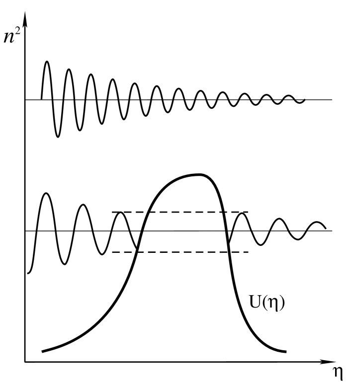
Figure 8: Effective potential $U(\eta)$.

After having formulated the initial conditions, the present day behaviour of $r_{n}$, $\phi_{n}$, $\theta_{n}$ (or, equivalently, the present day behaviour of $h_{n}$) is essentially all we need to find. The mean number of particles in a two-mode squeezed state is $2\sinh^{2}{r_{n}}$ for each $s$. This number determines the mean square amplitude of the gravitational wave field. The time behaviour of the squeeze angle $\phi_{n}$ determines the time dependence of the correlation functions of the field. The amplification (that is, the growth of $r_{n}$) governed by Eq. (54) is different for different wave numbers $n$. Therefore, the present day results depend on the present day frequency $\nu$ ($\nu={cn}/{2\pi a}$) measured in Hz.

In cosmology, the function $H\equiv\dot{a}/a\equiv ca^{\prime}/a^{2}$ is the time-dependent Hubble parameter. The function $l\equiv c/H$ is the time-dependent Hubble radius. The time-dependent wavelength of the mode $n$ is $\lambda=2\pi a/n$. The wavelength $\lambda$ has this universal definition in all regimes. In contrast, the $\nu$ defined as $\nu={cn}/{2\pi a}$ has the usual meaning of a frequency of an oscillating process only in the short-wavelength (high-frequency) regime of the mode $n$, that is, in the regime where $\lambda\ll l$. As we have seen above, the qualitative behaviour of the solutions to Eqs. (55), (58), depends crucially on the comparative values of $n$ and $a^{\prime}/a$, or, in other words, on the comparative values of $\lambda(\eta)$ and $l(\eta)$. This relationship is also crucial for the solutions to Eq. (54), as we shall see now.

In the short-wavelength regime, that is, during intervals of time when the wavelength $\lambda(\eta)$ is shorter than the Hubble radius $l(\eta)=a^{2}/a^{\prime}$, the term containing $n$ in (54) is dominant. The functions $\phi_{n}(\eta)$ and $\theta_{n}(\eta)$ are, $\phi_{n}=-n(\eta+\eta_{n})$, $\theta_{n}=\phi_{n}$ where $\eta_{n}$ is a constant. The factor $\cos 2\phi_{n}$ is a rapidly oscillating function of time, so the squeeze parameter $r_{n}$ stays practically a constant. This is the adiabatic regime for a given mode.

In the opposite, long-wavelength regime, the term $n$ can be neglected. The function $\phi_{n}$ is $\tan\phi_{n}(\eta)\approx\mbox{const}/a^{2}(\eta)$, and the squeeze angle quickly approaches one of the two values: $\phi_{n}=0$ or $\phi_{n}=\pi$ (analog of “phase bifurcation” [131, 132]). When the long-wavelength regime, for a given $n$, begins the squeeze parameter $r_{n}(\eta)$ grows with time according to

$$r_{n}(\eta)\approx ln\left[\frac{a(\eta)}{a_{*}}\right],$$ (60)

where $a_{*}$ is the value of $a(\eta)$ at $\eta_{*}$. The final value of $r_{n}$ is

$$r_{n}\approx ln\left[\frac{a_{**}}{a_{*}}\right],$$ (61)

where $a_{**}$ is the value of $a(\eta)$ at $\eta_{**}$, when the long-wavelength regime and amplification come to the end. It is important to emphasize that it is not a “sudden transition” from one cosmological era to another that is responsible for amplification, but the entire interval of the long-wavelength (non-adiabatic) regime.

After the end of amplification, the accumulated (and typically large) squeeze parameter $r_{n}$ stays approximately constant. The mode is again in the adiabatic regime. In course of the evolution, the complex functions ${\stackrel{{\scriptstyle s}}{{u}}}_{n}(\eta)+{\stackrel{{\scriptstyle s}}{{v}}}_{n}^{\ast}(\eta)$ become practically real, and one has ${\stackrel{{\scriptstyle s}}{{h}}}_{n}(\eta)\approx{\stackrel{{\scriptstyle s}}{{h}}}_{n}^{\ast}(\eta)\approx\frac{1}{a}e^{r_{n}}\cos\phi_{n}(\eta)$. Every amplified mode $n$ of the field (50) takes the form of a product of a function of time and a (random, operator-valued) function of spatial coordinates; the mode acquires a standing-wave pattern. The periodic dependence $\cos\phi_{n}(\eta)$ will be further discussed below.

It is clearly seen from the fundamental equations (54), (55), (58) that the final results depend only on $a(\eta)$. Equations do not ask us the names of our favorite cosmological prejudices, they ask us about the pump field $a(\eta)$. Conversely, from the measured relic gravitational waves, we can deduce the behaviour of $a(\eta)$, which is essentially the purpose of detecting the relic gravitons.

6.3 Cosmological Pump Field

With the chosen initial conditions, the final numerical results for relic gravitational waves depend on the concrete behaviour of the pump field represented by the cosmological scale factor $a(\eta)$. We know a great deal about $a(\eta)$. We know that $a(\eta)$ behaves as $a(\eta)\propto\eta^{2}$ at the present matter-dominated stage. We know that this stage was preceded by the radiation-dominated stage in which $a(\eta)\propto\eta$. At these two stages of evolution the functions $a(\eta)$ are simple power-law functions of $\eta$. What we do not know is the function $a(\eta)$ describing the initial stage of expansion of the very early Universe, that is, before the era of primordial nucleo-synthesis. It is convenient to parameterize $a(\eta)$ at this initial stage also by power-law functions of $\eta$. First, this is a sufficiently broad class of functions, which, in addition, allows us to find exact solutions to our fundamental equations. Second, it is known [124, 125, 9] that the pump fields $a(\eta)$ which have power-law dependence in terms of $\eta$, produce gravitational waves with simple power-law spectra in terms of $\nu$. These spectra are easy to analyze and discuss in the context of detection.

We model cosmological expansion by several successive eras. Concretely, we take $a(\eta)$ at the initial stage of expansion ($i$-stage) as

$$a(\eta)=l_{o}|\eta|^{1+\beta},$$ (62)

where $\eta$ grows from $-\infty$, and $1+\beta<0$. We will show later how the available observational data constrain the parameters $l_{o}$ and $\beta$. The $i$-stage lasts up to a certain $\eta=\eta_{1}$, $\eta_{1}<0$. To make our analysis more general, we assume that the $i$-stage was followed by some interval of the $z$-stage ($z$ from Zeldovich). It is known that an interval of evolution governed by the most “stiff” matter (effective equation of state $p=\epsilon$) advocated by Zeldovich, leads to a relative increase of gravitational wave amplitudes [124, 125, 9]. It is also known that the requirement of consistency of the graviton production with the observational restrictions does not allow the “stiff” matter interval to be too long [124, 125, 9, 133]. However, we want to investigate any interval of cosmological evolution that can be consistently included. In fact, the $z$-stage of expansion that we include is quite general. It can be governed by a “stiffer than radiation” [134] matter, as well as by a “softer than radiation” matter. It can also be simply a part of the radiation-dominated era. Concretely, we take $a(\eta)$ at the interval of time from $\eta_{1}$ to some $\eta_{s}$ ($z$-stage) in the form

$$a(\eta)=l_{o}a_{z}(\eta-\eta_{p})^{1+\beta_{s}},$$ (63)

where $1+\beta_{s}>0$. For the particular choice $\beta_{s}=0$, the $z$-stage reduces to an interval of expansion governed by the radiation-dominated matter. Starting from $\eta_{s}$ and up to $\eta_{2}$ the Universe was governed by the radiation-dominated matter ($e$-stage). So, in this interval of evolution, we take the scale factor in the form

$$a(\eta)=l_{o}a_{e}(\eta-\eta_{e}).$$ (64)

And, finally, from $\eta=\eta_{2}$ the expansion switched to the matter-dominated era ($m$–stage):

$$a(\eta)=l_{o}a_{m}(\eta-\eta_{m})^{2}.$$ (65)

A link between the arbitrary constants participating in Eqs. (62) - (65) is provided by the conditions of continuous joining of the functions $a(\eta)$ and $a^{\prime}(\eta)$ at points of transitions $\eta_{1}$, $\eta_{s}$, $\eta_{2}$.

We denote the present time by $\eta_{R}$ ($R$ from reception). This time is defined by the observationally known value of the present-day Hubble parameter $H(\eta_{R})$ and Hubble radius $l_{H}=c/{H(\eta_{R})}$. For numerical estimates we will be using $l_{H}\approx 2\times 10^{28}~{}{\rm cm}$. It is convenient to choose $\eta_{R}-\eta_{m}=1$, so that $a(\eta_{R})=2l_{H}$. The ratio

$$a(\eta_{R})/a(\eta_{2})\equiv\zeta_{2}$$

is believed to be around $\zeta_{2}=10^{4}$. We also denote

$$a(\eta_{2})/a(\eta_{s})\equiv\zeta_{s}~{},~{}~{}~{}a(\eta_{s})/a(\eta_{1})\equiv\zeta_{1}~{}.$$

With these definitions, all the constants participating in Eqs. (62) - (65) (except parameters $\beta$ and $\beta_{s}$ which should be chosen from other considerations) are being expressed in terms of $l_{H}$, $\zeta_{2}$, $\zeta_{s}$, and $\zeta_{1}$. For example,

$$|\eta_{1}|=\frac{|1+\beta|}{2\zeta_{2}^{\frac{1}{2}}\zeta_{s}{\zeta_{1}}^{\frac{1}{1+\beta_{s}}}}~{}.$$

The important constant $l_{o}$ is expressed as

$$l_{o}=bl_{H}\zeta_{2}^{\frac{\beta-1}{2}}\zeta_{s}^{\beta}{\zeta_{1}}^{\frac{\beta-\beta_{s}}{1+\beta_{s}}},$$ (66)

where $b\equiv 2^{2+\beta}/{|1+\beta|}^{1+\beta}$. Note that $b=1$ for $\beta=-2$. (This expression for $l_{o}$ may help to relate formulas written here with the equivalent treatment [135] which was given in slightly different notations.) The sketch of the entire evolution $a(\eta)$ is given in Fig. 9.

Figure 9: Scale factor $a(\eta)$.

We work with the spatially-flat models (48). At every instant of time, the energy density $\epsilon(\eta)$ of matter driving the evolution is related with the Hubble radius $l(\eta)$ by

$$\kappa\epsilon(\eta)=\frac{3}{l^{2}(\eta)},$$ (67)

where $\kappa=8\pi G/c^{4}$. For the case of power-law scale factors $a(\eta)\propto\eta^{1+\beta}$, the effective matter pressure $p(\eta)$ is related to the energy density $\epsilon(\eta)$ by the effective equation of state

$$p=\frac{1-\beta}{3(1+\beta)}\epsilon.$$ (68)

For instance, $p=0$ for $\beta=1$, $p=\frac{1}{3}\epsilon$ for $\beta=0$, $p=-\epsilon$ for $\beta=-2$, and so on. Each interval of the evolution (62)-(65) is governed by one of these equations of state.

In principle, the function $a(\eta)$ could be even more complicated than the one that we consider. It could even include an interval of early contraction, instead of expansion, leading to a “bounce” of the scale factor. In the case of a decreasing $a(\eta)$ the gravitational-wave equation can still be analyzed and the amplification is still effective [124, 125, 9]. However, the Einstein equations for spatially-flat models do not permit a regular “bounce” of $a(\eta)$ (unless $\epsilon$ vanishes at the moment of “bounce”). Possibly, a “bounce” solution can be realized in alternative theories, such as string-motivated cosmologies [136, 137, 138]. For a recent discussion of spectral slopes of gravitational waves produced in “bounce” cosmologies, see [139].

6.4 Solving Gravitational Wave Equations

The evolution of the scale factor $a(\eta)$ given by Eqs. (62) - (65) and sketched in Fig. 9 allows us to calculate the function $a^{\prime}/a$. This function is sketched in Fig. 10. In all theoretical generality, the left-hand-side of the barrier in Fig. 10 could also consist of several pieces, but we do not consider this possibility here. The graph also shows the important wave numbers $n_{H}$, $n_{2}$, $n_{s}$, $n_{1}$: $n_{H}$ marks the wave whose today’s wavelength $\lambda(\eta_{R})=2\pi a(\eta_{R})/n_{H}$ is equal to the Hubble radius $l_{H}$ today. With our parameterization $a(\eta_{R})=2l_{H}$, this wave-number is $n_{H}=4\pi$. $n_{2}$ marks the wave whose wavelength $\lambda(\eta_{2})=2\pi a(\eta_{2})/n_{2}$ at $\eta=\eta_{2}$ is equal to the Hubble radius $l(\eta_{2})$ at $\eta=\eta_{2}$. Since $\lambda(\eta_{R})/\lambda(\eta_{2})=(n_{2}/n_{H})[a(\eta_{R})/a(\eta_{2})]$ and $l(\eta_{R})/l(\eta_{2})=[a(\eta_{R})/a(\eta_{2})][a(\eta_{R})/a(\eta_{2})]^{1/2}$, this gives us $n_{2}/n_{H}=[a(\eta_{R})/a(\eta_{2})]^{1/2}=\zeta_{2}^{1/2}$. Working out in a similar fashion other ratios, we find

$$\frac{n_{2}}{n_{H}}=\zeta_{2}^{\frac{1}{2}},~{}~{}~{}\frac{n_{s}}{n_{2}}=\zeta_{s},~{}~{}\frac{n_{1}}{n_{s}}=\zeta_{1}~{}^{\frac{1}{1+\beta_{s}}}.$$ (69)

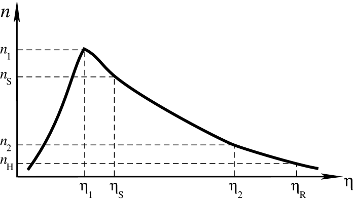
Figure 10: Function $a^{\prime}/a$ for the scale factor from Fig. 9.

Solutions to the gravitational wave equations exist for any $a(\eta)$. At intervals of power-law dependence $a(\eta)$, solutions to Eq. (55) have simple form of the Bessel functions. We could have found piece-wise exact solutions to Eq. (55) and join them in the transition points. However, we will use a much simpler treatment, which is sufficient for our purposes. We know that the squeeze parameter $r_{n}$ stays constant in the short-wavelength regimes and grows according to Eq. (60) in the long-wavelength regime. All modes start in the vacuum state, that is, $r_{n}=0$ initially. After the end of amplification, the accumulated value (61) stays constant up to today. To find today’s value of $e^{r_{n}}$ we need to calculate the ratio $a_{**}(n)/a_{*}(n)$. For every given $n$, the quantity $a_{*}$ is determined by the condition $\lambda(\eta_{*})=l(\eta_{*})$, whereas $a_{**}$ is determined by the condition $\lambda(\eta_{**})=l(\eta_{**})$.

Let us start from the mode $n=n_{1}$. For this wave number we have $a_{*}=a_{**}=a(\eta_{1})$, and therefore, $r_{n_{1}}=0$. The higher frequency modes, i.e. $n>n_{1}$ (above the barrier in Fig. 10), have never been in the amplifying regime, so we can write

$$e^{r_{n}}=1,~{}~{}n\geq n_{1}.$$ (70)

Let us now consider the modes $n$ in the interval $n_{1}\geq n\geq n_{s}$. For a given $n$ we need to know $a_{*}(n)$ and $a_{**}(n)$. Using Eq. (62) one has $a_{*}(n)/a_{*}(n_{1})=(n_{1}/n)^{1+\beta}$, and using Eq. (63) one finds $a_{**}(n)/a_{**}(n_{s})=(n_{s}/n)^{1+\beta_{s}}$. Therefore, one finds

$$\frac{a_{**}(n)}{a_{*}(n)}=\frac{a_{**}(n_{s})}{a_{*}(n_{1})}\left(\frac{n_{s}}{n}\right)^{1+\beta_{s}}\left(\frac{n}{n_{1}}\right)^{1+\beta}.$$

Since $a_{**}(n_{s})=a(\eta_{s})$, $a_{*}(n_{1})=a(\eta_{1})$, and $a(\eta_{s})/a(\eta_{1})=\zeta_{1}=(n_{1}/n_{s})^{1+\beta_{s}}$, we arrive at

$$\frac{a_{**}(n)}{a_{*}(n)}=\left(\frac{n}{n_{1}}\right)^{\beta-\beta_{s}}.$$

Repeating this analysis for other intervals of the decreasing $n$, we come to the conclusion that

$$e^{r_{n}} = \left(\frac{n}{n_{1}}\right)^{\beta-\beta_{s}},~{}~{}n_{1}\geq n\geq n_{s},$$

$$e^{r_{n}} = \left(\frac{n}{n_{s}}\right)^{\beta}\left(\frac{n_{s}}{n_{1}}\right)^{\beta-\beta_{s}},~{}~{}n_{s}\geq n\geq n_{2},$$

$$e^{r_{n}} = \left(\frac{n}{n_{2}}\right)^{\beta-1}\left(\frac{n_{2}}{n_{1}}\right)^{\beta}\left(\frac{n_{s}}{n_{1}}\right)^{-\beta_{s}},n_{2}\geq n\geq n_{H}.$$ (71)

The mnemonic rule of constructing $e^{r_{n}}$ at successive intervals of decreasing $n$ is simple. If the interval begins at $n_{x}$, one takes $(n/n_{x})^{\beta_{*}-\beta_{**}}$ and multiples with $e^{r_{n_{x}}}$, that is, with the previous interval’s value of $e^{r_{n}}$ calculated at the end of that interval $n_{x}$. For the function $a^{\prime}/a$ that we are working with, the $\beta_{*}$ is always $\beta$, whereas the $\beta_{**}$ takes the values $\beta_{s}$, $0$, $1$, at the successive intervals.

The modes with $n<n_{H}$ are still in the long-wavelength regime. For these modes, we should take $a(\eta_{R})$ instead of $a_{**}(n)$. Combining with $a_{*}(n)$, we find

$$e^{r_{n}}=\left(\frac{n}{n_{H}}\right)^{\beta+1}\left(\frac{n_{H}}{n_{2}}\right)^{\beta-1}\left(\frac{n_{2}}{n_{1}}\right)^{\beta}\left(\frac{n_{s}}{n_{1}}\right)^{-\beta_{s}},~{}n\leq n_{H}.$$ (72)

Formulas (70) - (72) give approximate values of $r_{n}$ for all $n$. The factor $e^{r_{n}}$ obeys the following inequalities is $e^{r_{n}}\geq 1$ for $n\leq n_{1}$, and $e^{r_{n}}\gg 1$ for $n\ll n_{1}$, and determines the mean square amplitude of the gravitational waves.

The mean value of the field $h_{ij}$ is zero at every moment of time $\eta$ and in every spatial point ${\bf x}$: $\langle 0|h_{ij}(\eta,{\bf x})|0\rangle=0$. The variance

$$\langle 0|h_{ij}(\eta,{\bf x})h^{ij}(\eta,{\bf x})|0\rangle~{}\equiv~{}\langle h^{2}\rangle$$

is not zero, and it determines the mean square amplitude of the generated field - the quantity of interest for the experiment. Taking the product of two expressions (50) one can show that

$$\langle h^{2}\rangle=\frac{C^{2}}{2\pi^{2}}\int\limits_{0}^{\infty}n\sum_{s=1}^{2}\Big{|}{\stackrel{{\scriptstyle s}}{{h}}}_{n}(\eta)\Big{|}^{2}~{}{\rm d}n\equiv\int\limits_{0}^{\infty}h^{2}(n,\eta)\frac{{\rm d}n}{n}~{}.$$ (73)

Using the representation (51), (52) in Eq. (73) one can also write

$$\langle h^{2}\rangle=\frac{C^{2}}{{\pi^{2}}a^{2}}\int\limits_{0}^{\infty}n{\rm d}n(\cosh 2{r_{n}}+\cos 2{\phi_{n}}\sinh 2{r_{n}}).$$ (74)

We can now consider the present era and use the fact that $e^{r_{n}}$ are large numbers for all $n$ in the interval of our interest $n_{1}\geq n\geq n_{H}$. Then, we can derive

$$h(n,\eta)\approx\frac{C}{\pi}\frac{1}{a(\eta_{R})}ne^{r_{n}}\cos\phi_{n}(\eta)=8\sqrt{\pi}\left(\frac{l_{Pl}}{l_{H}}\right)\left(\frac{n}{n_{H}}\right)e^{r_{n}}\cos\phi_{n}(\eta)~{}.$$ (75)

The quantity $h(n,\eta)$ is the dimensionless spectral amplitude of the field whose numerical value is determined by the calculated squeeze parameter $r_{n}$. The oscillatory factor $\cos\phi_{n}(\eta)$ reflects the squeezing (standing wave pattern) acquired by modes with $n_{1}>n>n_{H}$. For modes with $n<n_{H}$ this factor is approximately $1$. For high-frequency modes $n\gg n_{H}$ one has $\phi_{n}(\eta)\approx n(\eta-\eta_{n})\gg 1$, so that $h(n,\eta)$ makes many oscillations while the scale factor $a(\eta)$ is practically fixed at $a(\eta_{R})$.

The integral (74) extends formally from $0$ to $\infty$. Since $r_{n}\approx 0$ for $n\geq n_{1}$, the integral diverges at the upper limit. This is a typical ultra-violet divergence. It should be discarded (renormalized to zero) because it comes from the modes which have always been in their vacuum state. At the lower limit, the integral diverges, if $\beta\leq-2$. This is an infra-red divergence which comes from the assumption that the amplification process has started from infinitely remote time in the past. One can deal with this divergence either by introducing a lower frequency cut-off (equivalent to the finite duration of the amplification) or by considering only the parameters $\beta>-2$, in which case the integral is convergent at the lower limit. It appears that the available observational data (see below) favour this second option. The particular case $\beta=-2$ corresponds to the de Sitter evolution $a(\eta)\propto|\eta|^{-1}$. In this case, the $h(n)$ found in Eqs. (75), (72) does not depend on $n$. This is known as the Harrison-Zeldvich, or scale-invariant, spectrum.

The spectral amplitudes $h(n)$ can also be derived using the approximate solutions (56), (57) to the wave equation (55). This method gives exactly the same, as in Eqs. (75), (70) - (72) numerical values of $h(n)$, but does not reproduce the oscillatory factor $\cos\phi_{n}(\eta)$.

One begins with the initial spectral amplitude $h_{i}(n)$ defined by quantum normalization: $h_{i}(n)=8\sqrt{\pi}(l_{Pl}/\lambda_{i})$. This is the amplitude of the mode $n$ at the moment $\eta_{*}$ of entering the long wavelength regime, i.e. when the mode’s wavelength $\lambda_{i}$ is equal to the Hubble radius $l(\eta_{*})$. For $\lambda_{i}$ one derives

$$\lambda_{i}=\frac{1}{b}l_{o}\left(\frac{n_{H}}{n}\right)^{2+\beta}.$$ (76)

Thus, we have

$$h_{i}(n)=A\left(\frac{n}{n_{H}}\right)^{2+\beta},$$ (77)

where $A$ denotes the constant

$$A=b8\sqrt{\pi}\frac{l_{P}l}{l_{o}}~{}.$$ (78)

The numbers $h_{i}(n)$ are defined at the beginning of the long-wavelength regime. In other words, they are given along the left-hand-side slope of the barrier in Fig. 10. We want to know the final numbers (spectral amplitudes) $h(n)$ which describe the field today, at $\eta_{R}$.

According to the dominant solution $h_{n}(\eta)=\mbox{const,}$ of the long-wavelength regime (see Eq. (59)), the initial amplitude $h_{i}(n)$ stays practically constant up to the end of the long-wavelength regime at $\eta_{**}$, that is, up to the right-hand-side slope of the barrier. (The second term in Eq. (57) could be important only at the $z$-stage and only for parameters $\beta_{s}\leq-(1/2)$, which correspond to the effective equations of state $p\geq\epsilon$. In order to keep the analysis simple, we do not consider those cases.) After the completion of the long-wavelength regime, the amplitudes decrease adiabatically in proportion to $1/a(\eta)$, up to the present time. Thus, we have

$$h(n)=A\left(\frac{n}{n_{H}}\right)^{2+\beta}\frac{a_{**}(n)}{a(\eta_{R})}.$$ (79)

Let us start from the lower end of the spectrum, $n\leq n_{H}$, and go upward in $n$. The modes $n\leq n_{H}$ have not started yet the adiabatic decrease of the amplitude, so we have

$$h(n)=A\left(\frac{n}{n_{H}}\right)^{2+\beta},~{}~{}n\leq n_{H}.$$ (80)

Now consider the interval $n_{2}\geq n\geq n_{H}$. At this interval, the $a_{**}(n)/a(\eta_{R})$ scales as $(n_{H}/n)^{2}$, so we have

$$h(n)=A\left(\frac{n}{n_{H}}\right)^{\beta},~{}~{}n_{2}\geq n\geq n_{H}.$$ (81)

At the interval $n_{s}\geq n\geq n_{2}$ the ratio $a_{**}(n)/a(\eta_{R})=[a_{**}(n)/a(\eta_{2})][a(\eta_{2})/a(\eta_{R})]$ scales as $(n_{2}/n)(n_{H}/n_{2})^{2}$, so we have

$$h(n)=A\left(\frac{n}{n_{H}}\right)^{1+\beta}\frac{n_{H}}{n_{2}},~{}~{}n_{s}\geq n\geq n_{2}.$$ (82)

Repeating the same analysis for the interval $n_{1}\geq n\geq n_{s}$ we find

$$h(n)=A\left(\frac{n}{n_{H}}\right)^{1+\beta-\beta_{s}}\left(\frac{n_{s}}{n_{H}}\right)^{\beta_{s}}\frac{n_{H}}{n_{2}},~{}~{}n_{1}\geq n\geq n_{s}.$$ (83)

It is seen from Eq. (83) that an interval of the $z$-stage with $\beta_{s}<0$ (the already imposed restrictions require also $(-1/2)<\beta_{s}$) bends the spectrum $h(n)$ upwards, as compared with Eq. (82), for larger $n$. If one recalls the relationship (66) between $l_{o}$ and $l_{H}$ and uses (6.4), (72) in Eq. (75) one arrives exactly at Eqs. (80)-(83) up to the oscillating factor $\cos\phi_{n}(\eta)$.

Different parts of the barrier in Fig. 10 are responsible for amplitudes and spectral slopes at different intervals of $n$. The sketch of the generated spectrum $h(n)$ in conjunction with the form of the barrier is shown in Fig. 11.

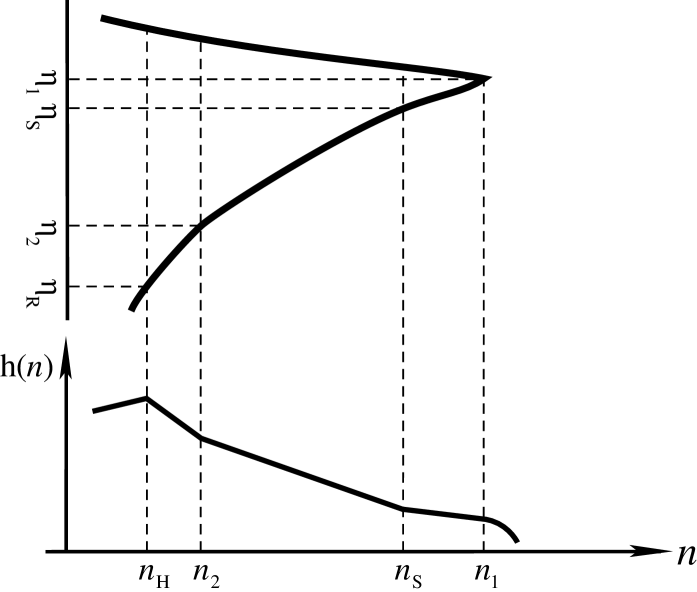
Figure 11: Amplitudes and spectral slopes of $h(n)$ are determined by different parts of the barrier $a^{\prime}/a$.

The present day frequency of the oscillating modes, measured in Hz, is defined as $\nu=cn/2\pi a(\eta_{R})$. The lowest frequency (Hubble frequency) is $\nu_{H}=c/l_{H}$. For numerical estimates we will be using $\nu_{H}\approx 10^{-18}$ Hz. The ratios of $n$ are equal to the ratios of $\nu$, so that, for example, $n/n_{H}=\nu/\nu_{H}$. For high-frequency modes we will now often use the ratios of $\nu$ instead of ratios of $n$.

In addition to the spectral amplitudes $h(n)$ the generated field can be also characterized by the spectral energy density parameter $\Omega_{g}(n)$. The energy density $\epsilon_{g}$ of the gravitational wave field is

$$\kappa\epsilon_{g}=\frac{1}{4}h^{ij}_{~{},0}h_{ij,0}=\frac{1}{4a^{2}}{h^{ij}}^{\prime}{h_{ij}}^{\prime}.$$

The mean value $\langle 0|\epsilon_{g}(\eta,{\bf x})|0\rangle$ is given by

$$\kappa\langle\epsilon_{g}\rangle=\frac{1}{4a^{2}}\frac{C^{2}}{2\pi^{2}}\int\limits_{0}^{\infty}n\sum_{s=1}^{2}\Big{|}{{\stackrel{{\scriptstyle s}}{{h}}}}^{\prime}_{n}(\eta)\Big{|}^{2}~{}{\rm d}n.$$ (84)

For high-frequency modes, it is only the factor $e^{\pm in\eta}$ that needs to be differentiated by $\eta$. After averaging out the oscillating factors, one gets $\Big{|}{{\stackrel{{\scriptstyle s}}{{h}}}}^{\prime}_{n}\Big{|}^{2}=n^{2}\Big{|}{\stackrel{{\scriptstyle s}}{{h}}}_{n}\Big{|}^{2}$, so that

$$\kappa\langle\epsilon_{g}\rangle=\frac{1}{4a^{2}}\int\limits_{0}^{\infty}n^{2}h^{2}(n)\frac{{\rm d}n}{n}.$$ (85)

In fact, the high-frequency approximation, that has been used, permits integration over lower $n$ only up to $n_{H}$. And the upper limit, as was discussed above, is in practice $n_{1}$, not infinity. The parameter $\Omega_{g}$ is defined as $\Omega_{g}=\langle\epsilon_{g}\rangle/\epsilon$, where $\epsilon$ is given by Eq. (67) (critical density). So, we derive

$$\Omega_{g}=\int\limits_{n_{H}}^{n_{1}}\Omega_{g}(n)\frac{{\rm d}n}{n}=\int\limits_{\nu_{H}}^{\nu_{1}}\Omega_{g}(\nu)\frac{{\rm d}\nu}{\nu}$$

and

$$\Omega_{g}(\nu)=\frac{\pi^{2}}{3}h^{2}(\nu)\left(\frac{\nu}{\nu_{H}}\right)^{2}.$$ (86)

The dimensionless quantity $\Omega_{g}(\nu)$ is useful because it allows us to quickly evaluate the cosmological importance of the generated field in a given frequency interval. However, the primary and more universal concept is $h(\nu)$, not $\Omega_{g}(\nu)$. It is the field, not its energy density, that is directly measured by the gravity-wave detector. One should also note that some authors use quite a misleading definition $\Omega_{g}(f)=(1/\rho_{c})(d\rho_{gw}/d\ln f)$ which suggests differentiation of the gravity-wave energy density by frequency. This would be incorrect and could cause disagreements in numerical values of $\Omega_{g}$. Whenever we use $\Omega_{g}(\nu)$, we mean relationship (86); and for order of magnitude estimates one can use [124, 125, 9]:

$$\Omega_{g}(\nu)\approx h^{2}(\nu)\left(\frac{\nu}{\nu_{H}}\right)^{2}.$$ (87)

6.5 Theoretical and Observational Constraints

The entire theoretical approach is based on the assumption that a weak quantized gravity-wave field interacts with a classical pump field. We should follow the validity of this approximation throughout the analysis. The pump field can be treated as a classical gravitational field as long as the driving energy density $\epsilon$ is smaller than the Planck energy density, or, in other words, as long as the Hubble radius $l(\eta)$ is greater than the Planck length $l_{Pl}$. This is a restriction on the pump field, but it can be used as a restriction on the wavelength $\lambda_{i}$ of the gravity-wave mode $n$ at the time when it enters the long-wavelength regime. If $l(\eta_{*})>l_{Pl}$, then $\lambda_{i}>l_{Pl}$. The $\lambda_{i}$ is given by Eq. (76). So, we need to ensure that

$$b\frac{l_{Pl}}{l_{o}}\left(\frac{\nu}{\nu_{H}}\right)^{2+\beta}<1.$$

At the lowest-frequency end $\nu=\nu_{H}$ this inequality gives $b(l_{Pl}/l_{o})<1$. In fact, the observational constraints (see below) give a stronger restriction:

$$b\frac{l_{Pl}}{l_{o}}\approx 10^{-6},$$ (88)

which we accept. Then, at the highest-frequency end $\nu=\nu_{1}$ we need to satisfy

$$\left(\frac{\nu_{1}}{\nu_{H}}\right)^{2+\beta}<10^{6}.$$ (89)

Let us now turn to the generated spectral amplitudes $h(\nu)$. According to Eq. (80) we have $h(\nu_{H})\approx b8\sqrt{\pi}(l_{Pl}/l_{o})$. The measured microwave background anisotropies, which we discuss below, require this number to be at the level of $10^{-5}$, which gives the already mentioned Eq. (88). The quantity $h(\nu_{1})$ at the highest frequency $\nu_{1}$ is given by Eq. (83):

$$h(\nu_{1})=b8\sqrt{\pi}\frac{l_{Pl}}{l_{o}}\left(\frac{\nu_{1}}{\nu_{H}}\right)^{1+\beta-\beta_{s}}\left(\frac{\nu_{s}}{\nu_{H}}\right)^{\beta_{s}}\frac{\nu_{H}}{\nu_{2}}.$$

Using Eq. (66) this expression for $h(\nu_{1})$ can be rewritten as

$$h(\nu_{1})=8\sqrt{\pi}\frac{l_{Pl}}{l_{H}}\frac{\nu_{1}}{\nu_{H}}=8\sqrt{\pi}\frac{l_{Pl}}{\lambda_{1}},$$ (90)

where $\lambda_{1}=c/\nu_{1}$. This last expression for $h(\nu_{1})$ is not surprising: the modes with $\nu\geq\nu_{1}$ are still in the vacuum state, so the numerical value of $h(\nu_{1})$ is determined by quantum normalization.

All the amplified modes have started with small initial amplitudes $h_{i}$, at the level of zero-point quantum fluctuations. These amplitudes are also small today, since the $h_{i}$ could only stay constant or decrease. However, even these relatively small amplitudes should obey observational constraints. We do not want the $\Omega_{g}$ in the high-frequency modes, which might affect the rate of the primordial nucleosynthesis, to exceed the level of $10^{-5}$. This means that $\Omega_{g}(\nu_{1})$ cannot exceed the level of $10^{-6}$ or so. The use of Eq. (86) in combination with $\Omega_{g}(\nu_{1})\approx 10^{-6}$ and $h(\nu_{1})$ from Eq. (90), gives us the highest allowed frequency $\nu_{1}\approx 3\times 10^{10}$ Hz. We will use this value of $\nu_{1}$ in our numerical estimates. Returning with this value of $\nu_{1}$ to Eq. (89) we find that the parameter $\beta$ can only be $\beta\leq-1.8$. We will be treating $\beta=-1.8$ as the upper limit for the allowed values of $\beta$.

We can now check whether the accepted parameters leave room for the postulated $z$-stage with $\beta_{s}<0$. Using Eq. (66) we can rewrite Eq. (88) in the form

$$10^{-6}\frac{l_{H}}{l_{Pl}}=\left(\frac{\nu_{1}}{\nu_{H}}\right)^{-\beta}\left(\frac{\nu_{1}}{\nu_{s}}\right)^{\beta_{s}}\frac{\nu_{2}}{\nu_{H}}.$$ (91)

We know that $\nu_{2}/\nu_{H}=10^{2}$ and $\nu_{1}/\nu_{s}$ is not smaller than $1$. Substituting all the numbers in Eq. (91) one can find that this equation cannot be satisfied for the largest possible $\beta=-1.8$. In the case $\beta=-1.9$, Eq. (91) is only marginally satisfied, in the sense that a significant deviation from $\beta_{s}=0$ toward negative $\beta_{s}$ can only last for a relatively short time. For instance, one can accommodate $\beta_{s}=-0.4$ and $\nu_{s}=10^{8}$ Hz. On the other hand, if one takes $\beta=-2$, a somewhat longer interval of the $z$-stage with $\beta_{s}<0$ can be included. For instance, Eq. (91) is satisfied if one accepts $\nu_{s}=10^{-4}$ Hz and $\beta_{s}=-0.3$. This allows us to slightly increase $h(\nu)$ in the interval $\nu_{s}<\nu<\nu_{1}$, as compared with the values of $h(\nu)$ reached in the more traditional case $\beta=-2$, $\beta_{s}=0$. In what follows, we will consider consequences of this assumption for the prospects of detection of the produced gravitational wave signal. Finally, let us see what the available information on the microwave background anisotropies [140, 141] allows us to conclude about the parameters $\beta$ and $l_{o}$.

Usually, cosmologists operate with the spectral index ${\rm n}$ (not to be confused with the wave number $n$) of primordial cosmological perturbations. Taking into account the way in which the spectral index ${\rm n}$ is defined, one can relate ${\rm n}$ with the spectral index $\beta+2$ that shows up in Eq. (80). The relationship between them is ${\rm n}=2\beta+5$. This relationship is valid independently of the nature of cosmological perturbations. In particular, it is valid for density perturbations, in which case the $h(n)$ of Eq. (80) is the dimensionless spectral amplitude of metric perturbations associated with density perturbations. If primordial gravitational waves and density perturbations were generated by the mechanism that we discuss here (an assumption that is likely to be true) then the parameter $\beta$ that participates in the spectral index is the same as the one that participates in the scale factor of Eq. (62). Primordial gravitational waves and primordial density perturbations with the same spectral index $\beta+2$ produce approximately the same lower-order multiple distributions of large-scale anisotropies.

The evaluation of the spectral index ${\rm n}$ of primordial perturbations have resulted in ${\rm n}=1.2\pm 0.3$ [141] or even in a somewhat higher value. A recent analysis [142] of all available data favors ${\rm n}=1.2$ and the quadrupole contribution of gravitational waves twice as large as that of density perturbations. One can interpret these evaluations as an indication that the true value of ${\rm n}$ lies somewhere near ${\rm n}=1.2$ (hopefully, the planned new observational missions will determine this index more accurately). This gives us the parameter $\beta$ somewhere near $\beta=-1.9$. We will be using $\beta=-1.9$ in our estimates below, as the observationally preferred value. The parameter $\beta$ can be somewhat larger than $\beta=-1.9$. However, as we already discussed, the value $\beta=-1.8$ (${\rm n}=1.4$) is the largest one for which the entire approach is well posed. The Harrison-Zeldovich spectral index ${\rm n}=1$ corresponds to $\beta=-2$.

The observed quadrupole anisotropy of the microwave background radiation is at the level $\delta T/T\approx 10^{-5}$. The quadrupole anisotropy that would be produced by the spectrum (80) - (83) is mainly accounted for by the wave numbers near $n_{H}$. Thus, the numerical value of the quadrupole anisotropy produced by relic gravitational waves is approximately equal to $A$. According to general physical considerations and detailed calculations [143, 144, 145], the metric amplitudes of long-wavelength gravitational waves and density perturbations generated by the discussed amplification mechanism are of the same order of magnitude. Therefore, they contribute roughly equally to the anisotropy at lower multipoles. This gives us the estimate $A\approx 10^{-5}$, that we have already used in Eq. (88). It is not yet proven observationally that a significant part of the observed anisotropies at lower multipoles is indeed provided by relic gravitational waves, but we can at least assume this with some degree of confidence. It is likely that the future measurements of the microwave background radiation, and especially its polarization, will help us verify this theoretical conclusion.

Combining all the evaluated parameters together, we show in Fig. 12 the expected spectrum of $h(\nu)$ for the case $\beta=-1.9$. A small allowed interval of the $z$-stage is also included. The intervals of the spectrum accessible to space- and ground-based interferometers are indicated by vertical lines.

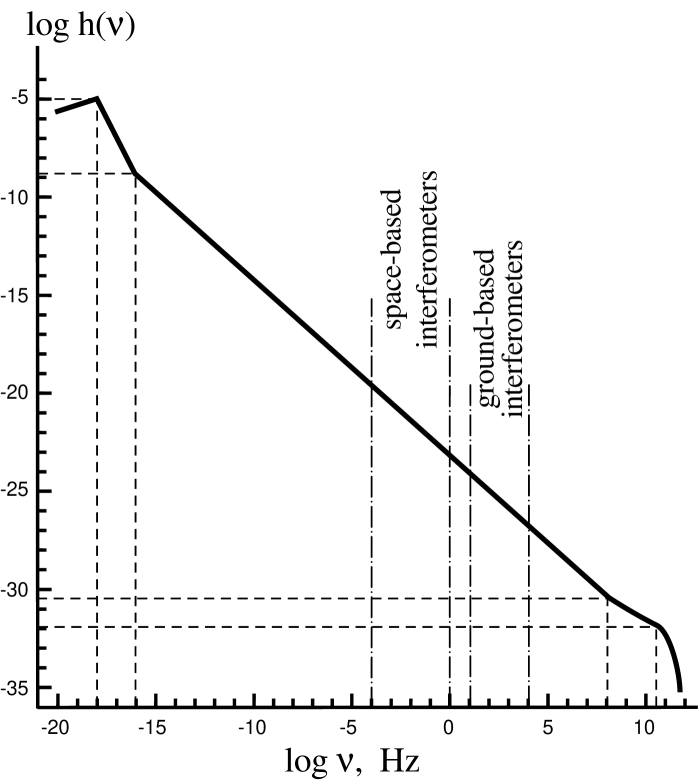
Figure 12: Expected spectrum $h(\nu)$ for the case $\beta=-1.9$.

It is necessary to note [143, 144, 145, 146] that a confirmation of any ${\rm n}>1$ ($\beta>-2$) will mean that the very early Universe was not driven by a scalar field - the cornerstone of inflationary considerations. Indeed, the ${\rm n}>1$ ($\beta>-2$) requires the effective equation of state at the initial stage of expansion to be $\epsilon+p<0$ (see Eq. (68)). But this requirement cannot be accommodated by any scalar field $\varphi(t)$ whatever the scalar field potential $V(\varphi)$ may be. The energy density of the scalar field is $\epsilon={\dot{\varphi}}^{2}/2+V(\varphi)$, whereas its pressure is $p={\dot{\varphi}}^{2}/2-V(\varphi)$, so that $\epsilon+p$ cannot be negative. The available data do not prove yet that ${\rm n}>1$, but this possibility seems likely.

It is also necessary to comment on a certain damage to gravitational wave research that was inflicted by the so called “standard inflationary result”. The “standard inflationary result” predicts infinitely large amplitudes of density perturbations $\delta\rho/\rho$ in the interval of spectrum with the Harrison-Zeldovich slope ${\rm n}=1$ ($\beta=-2$): $\delta\rho/\rho\propto V^{3/2}/V^{\prime}\propto 1/\sqrt{1-{\rm n}}$. The metric (curvature) perturbations $h_{S}$ accompanying $\delta\rho/\rho$ are also predicted to be infinitely large, in the same proportion. Inflationary literature conceals this predicted infinity of density perturbations by writing the ratio of the gravitational wave amplitude $h_{T}$ to the scalar metric amplitude $h_{S}$: $h_{T}/h_{S}\approx 7\sqrt{1-{\rm n}}$, and declaring that the contribution of gravitational waves to the cosmic microwave background (CMB) anisotropies should be zero, or almost zero, for ${\rm n}\approx 1$. Thus, the “standard” inflationary theory shifts the spectrum of relic gravitational waves, similar in shape to the one shown in Fig. 12, down by many orders of magnitude. This claim has incorrectly led to discarding the gravitational wave contribution in the analysis of CMB data. Although one of the recent best fits to the available data indicates the presence of the gravitational wave contribution [147] this fit has been ignored. For many years, inflationary theorists claimed that their arbitrarily large density perturbations were caused by the “big amplification during reheating”. It is now universally accepted that this explanation is false. The scalar metric perturbation, similarly to the gravitational wave perturbation (see Eq. (59)), remains constant during the long wavelength regime, that is, its numerical value does not change on the way from the first “Hubble-radius-crossing” to the second “Hubble-radius-crossing”. This fact is also reflected in the constancy of the so-called “conserved” gauge-invariant quantity $\zeta$, which is in the center of inflationary analysis (see, for example, [148]). Since the “standard” inflationary theory predicts arbitrarily large numerical value of $\zeta$, and this quantity is “conserved” during the evolution, this arbitrarily large number must have been postulated from the very beginning, as quantum normalization. This happens if one incorrectly assigns the quantum normalization to the scalar field perturbations alone, as if they were a free scalar test field in the De-Sitter space-time. Then, the quantity $\zeta$, calculated from the perturbed Einstein equations, is arbitrarily large at the first “Hubble-radius-crossing”, and this number is being transmitted to the second “Hubble-radius-crossing”. In reality, however, scalar field perturbations are always coupled to metric (gravitational field) perturbations. The correct quantization of the combined degree of freedom renders the scalar metric (curvature) perturbation $h_{S}$ finite and small, and of the same order of magnitude as gravitational wave perturbation $h_{T}$. The inflationary formula for $\delta\rho/\rho$ is incorrect in that it misses the dimensionless factor $\sqrt{-\dot{H}/H^{2}}$ which cancels out the zero in the denominator and makes the generated density perturbations finite and small, even in the interval of spectrum with the Harrison-Zeldovich slope. The “standard inflationary result” is in a severe conflict not only with theory but with observations too: when the observers marginalize their data to ${\rm n}=1$ (enforce this value of ${\rm n}$ in data analysis) they find finite and small density perturbations, instead of infinitely large perturbations predicted by inflationary theorists. [For analytical expressions of the “standard inflationary result” see inflationary articles, including recent reviews. For graphical illustration of the divergent density perturbations and quadrupole anisotropies, predicted by inflationary theorists, see, for example, [149]. For critical analysis and disagreement with the “standard inflationary result” see [143, 144, 145]]. The most recent articles dealing with perturbations in quasi-deSitter models rightly emphasize the expected substantial contribution of gravitational waves to the large scale CMB anisotropies [150]. In short, general relativity and quantum field theory do not produce the “standard inflationary result”.

6.6 Detectability of Relic Gravitational Waves

We switch now from cosmology to prospects of detecting the predicted relic gravitational waves. The ground-based [15, 14, 151] and space-based [16, 152] laser interferometers (see also [153, 154, 155]) will be in the focus of our attention. We use laboratory frequencies $\nu$ and intervals of laboratory time $t$ $(c{\rm d}t=a(\eta_{R}){\rm d}\eta)$. Formulas (82) and (83), with $A=10^{-5}$, $\nu_{2}/\nu_{H}=10^{2}$, and the oscillating factor restored, can be written as

$$h(\nu,t)\approx 10^{-7}\cos[2\pi\nu(t-t_{\nu})]\left(\frac{\nu}{\nu_{H}}\right)^{\beta+1},~{}\nu_{2}\leq\nu\leq\nu_{s}$$ (92)

and

$$h(\nu,t)\approx 10^{-7}\cos[2\pi\nu(t-t_{\nu})]\left(\frac{\nu}{\nu_{H}}\right)^{1+\beta-\beta_{s}}\left(\frac{\nu_{s}}{\nu_{H}}\right)^{\beta_{s}}.~{}~{}\nu_{s}\leq\nu\leq\nu_{1}$$ (93)

where the deterministic (not random) constant $t_{\nu}$ does not vary significantly from one frequency to another at the intervals $\Delta\nu\approx\nu$. The explicit time dependence of the spectral variance $h^{2}(\nu,t)$ of the field, or, in other words, the explicit time dependence of the (zero-lag) temporal correlation function of the field at every given frequency, demonstrates that we are dealing with a non-stationary process (a consequence of squeezing and severe reduction of the phase uncertainty). We will first ignore the oscillating factor and will compare the predicted amplitudes with the sensitivity curves of advanced detectors. The potential reserve of improving the SNR by exploiting squeezing will be discussed later.

Let us start from the Laser Interferometer Space Antenna (LISA) [16]. The instrument will be most sensitive in the interval, roughly, from $10^{-3}$ Hz to $10^{-1}$ Hz, and will be reasonably sensitive in a broader range, up to frequencies $10^{-4}$ Hz and 1 Hz. The sensitivity graph of LISA to a stochastic background is usually plotted under the assumption of a 1-year observation time, that is, the root-mean-square (r.m.s.) instrumental noise is being evaluated in frequency bins $\Delta\nu=3\times 10^{-8}$ Hz around each frequency $\nu$. We need to rescale our predicted amplitude $h(\nu)$ to these bins.

The mean square amplitude of the gravitational wave field is given by the integral (73). Thus, the r.m.s. amplitude in the band $\Delta\nu$ centered at a given frequency $\nu$ is given by the expression

$$h(\nu,\Delta\nu)=h(\nu)\sqrt{\frac{\Delta\nu}{\nu}}.$$ (94)

We use Eqs. (92), (93) and calculate expression (94) assuming $\Delta\nu=3\times 10^{-8}$ Hz. The results are plotted in Fig. 13. Formula (92) has been used throughout the covered frequency interval for the realistic case $\beta=-1.9$ and for the extreme case $\beta=-1.8$. The line marked $z$-model describes the signal produced in the composite model with $\beta=-2$ up to $\nu_{s}=10^{-4}$ Hz (formula (92)) and then followed by formula (93) with $\beta_{s}=-0.3$. This model gives the signal a factor of $3$ higher at $\nu=10^{-3}$ Hz, than the model $\beta=-2$ extrapolated down to this frequency.

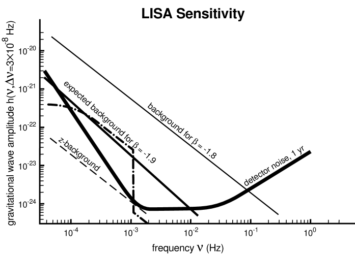
Figure 13: Expected spectrum $\beta=-1.9$ and other possible spectra in comparison with the LISA sensitivity.

There is no doubt that the signal $\beta=-1.8$ would be easily detectable even with a single instrument. The signal $\beta=-1.9$ is marginally detectable, with the SNR around $3$ or so, in a quite narrow frequency interval near and above the frequency $3\times 10^{-3}$ Hz. However, at lower frequencies one would need to be concerned with the possible gravitational wave noise from unresolved binary stars in our Galaxy (see Section 5). The further improvement of the expected LISA sensitivity by a factor of $3$ may prove to be crucial for a confident detection of the predicted signal with $\beta=-1.9$.

Let us now turn to the ground-based interferometers operating in the interval from 10 Hz to $10^{4}$ Hz. The best sensitivity is reached in the band around $\nu=10^{2}$ Hz. We take this frequency as the representative frequency for comparison with the predicted signal. We will work directly in terms of the dimensionless quantity $h(\nu)$. If necessary, the r.m.s. amplitude per Hz^1/2 at a given $\nu$ can be found simply as $h(\nu)/{\sqrt{\nu}}$. The instrumental noise will also be quoted in terms of the dimensionless quantity $h_{ex}(\nu)$.

The expected sensitivity of the initial instruments at $\nu=10^{2}$ Hz is $h_{ex}=10^{-21}$ or better. The theoretical prediction at this frequency, following from (92), (93) with $\beta_{s}=0$, is $h_{th}=10^{-23}$ for $\beta=-1.8$, and $h_{th}=10^{-25}$ for $\beta=-1.9$. Therefore, the gap between the signal and noise levels is from 2 to 4 orders of magnitude. The expected sensitivity of the advanced interferometers, such as LIGO-II [17], can be as high as $h_{ex}=10^{-23}$. In this case, the gap vanishes for the $\beta=-1.8$ signal and reduces to 2 orders of magnitude for the $\beta=-1.9$ signal. Fig. 14 illustrates the expected signal in comparison with the LIGO-II sensitivity. Since the signal lines are plotted in terms of $h(\nu)$, the LISA sensitivity curve (shown for periodic sources) should be raised and adjusted in accordance with Fig. 13.

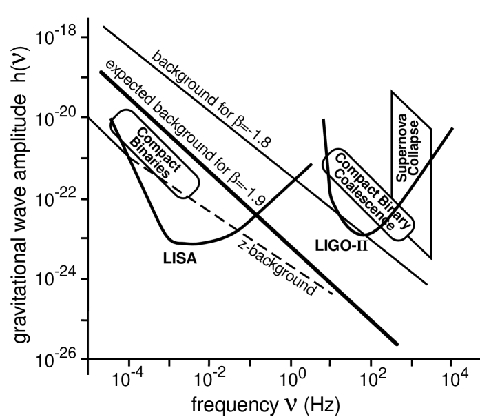
Figure 14: Full spectrum $h(\nu)$ accessible to laser interferometers.

A signal below noise can be detected if the outputs of two or more detectors can be cross correlated. (For the early estimates of detectability of relic gravitational waves see [156].) The cross correlation will be possible for ground-based interferometers, several of which are currently under construction. The gap between the signal and the noise levels should be covered by a sufficiently long observation time $\tau$. The duration $\tau$ depends on whether the signal has any temporal signature known in advance, or not. We start from the assumption that no temporal signatures are known in advance. In other words, we first ignore the squeezed nature of the relic background and work under the assumption that the squeezing cannot be exploited to our advantage.

The response of an instrument to the incoming radiation is $s(t)=F_{ij}h^{ij}$ where $F_{ij}$ depends on the position and orientation of the instrument. Since the $h^{ij}$ is a quantum-mechanical operator (see Eq. (50)) we need to calculate the mean value of a quadratic quantity. The mean value of the cross correlation of responses from two instruments $\langle 0|s_{1}(t)s_{2}(t)|0\rangle$ will involve the overlap reduction function [157, 158, 159, 160], which we assume to be not much smaller than $1$ [159]. The SNR in the measurement of the amplitude of a signal with no specific known features increases as $(\tau\nu)^{1/4}$, where $\nu$ is some characteristic central frequency (for more detail see Sec. 8).

We apply the guaranteed law $(\tau\nu)^{1/4}$ to initial and advanced instruments at the representative frequency $\nu=10^{2}$ Hz. This law requires a reasonably short time $\tau=10^{6}~{}{\rm sec}$ in order to improve the $S/N$ in initial instruments by two orders of magnitude and to reach the level of the signal with extreme spectral index $\beta=-1.8$. The longer integration time or a better sensitivity will make the $S/N$ larger than 1. In the case of a realistic spectral index $\beta=-1.9$ the remaining gap of 4 orders of magnitude can be covered by the combination of a significantly better sensitivity and a longer observation time (not necessarily in one non-interrupted run). The sensitivity of the advanced laser interferometers, such as LIGO II, at the level $h_{ex}=10^{-23}$ and the same observation time $\tau=10^{6}~{}{\rm sec}$ would be sufficient for reaching the level of the predicted signal with $\beta=-1.9$.

An additional increase of $S/N$ can be achieved if the statistical properties of the signal can be properly exploited. Squeezing is automatically present at all frequencies from $\nu_{H}$ to $\nu_{1}$. The squeeze parameter $r$ is larger in gravitational waves of cosmological scales, and possibly the periodic structure in Eq. (75) can be better revealed at those scales. However, we are interested here in frequencies accessible to ground based interferometers, say, in the interval 30–100 Hz. If our intention were to monitor one given frequency $\nu$ from the beginning of its oscillating regime and up till now, then, in order to avoid the destructive interference from neighbouring modes during all that time, the frequency resolution of the instrument should have been incredibly narrow, of the order of $10^{-18}$ Hz. Certainly, this is not something what we can, or intend to do. Although the amplitudes of the waves have adiabatically decreased and their frequencies redshifted since the beginning of their oscillating regime, the general statistical properties of the discussed signal are essentially the same now as they were $10$ years after the big bang or will be $1$ million years from now.

The periodic structure (92) may survive at some level in the instrumental window of sensitivity from $\nu_{min}$ (minimal frequency) to $\nu_{max}$ (maximal frequency). The mean square value of the field in this window is

$$\int\limits_{\nu_{min}}^{\nu_{max}}h^{2}(\nu,t)\frac{{\rm d}\nu}{\nu}=10^{-14}\frac{1}{{\nu_{H}}^{2\beta+2}}\int\limits_{\nu_{min}}^{\nu_{max}}\cos^{2}[2\pi\nu(t-t_{\nu})]\nu^{2\beta+1}{\rm d}\nu~{}.$$ (95)

Because of the strong dependence of the integrand on frequency, $\nu^{-2.6}$ or $\nu^{-2.8}$, the value of the integral (95) is determined by its lower limit. Apparently, the search through the data should be based on the periodic structure that may survive at $\nu=\nu_{min}$. As an illustration, one can consider such a narrow interval $\Delta\nu=\nu_{max}-\nu_{min}$ that the integral (95) can be approximated by the formula

$$\int\limits_{\nu_{min}}^{\nu_{max}}h^{2}(\nu,t)\frac{{\rm d}\nu}{\nu}\approx 10^{-14}\left(\frac{\nu_{min}}{{\nu_{H}}}\right)^{2\beta+2}\left(\frac{\Delta\nu}{\nu_{min}}\right)\cos^{2}[2\pi\nu_{min}(t-t_{min})]~{}.$$

Clearly, the correlation function is strictly periodic and its structure is known in advance, in contrast to other possible signals. This is a typical example of using the a priori information. Ideally, the gain in $S/N$ can grow as $(\tau\nu_{min})^{1/2}$. This would significantly reduce the required observation time $\tau$. For a larger $\Delta\nu$, even an intermediate gain between the guaranteed law $(\tau\nu)^{1/4}$ and the law $(\tau\nu)^{1/2}$, from the matched filtering technique, would help. This could potentially make the signal with $\beta=-1.9$ measurable even by the initial laser interferometers. A straightforward application of (95) exploiting squeezing may not be possible, as argued in a recent study [161], but more sophisticated methods are not excluded.

For frequency intervals covered by bar detectors and electromagnetic detectors, the expected results follow from the same formulas (92), (93) and have been briefly discussed elsewhere [156, 135].

6.7 Conclusion

It would be strange, if the predicted signal at the level corresponding to $\beta=-1.9$ were not seen by the instruments capable of its detection. There aren’t so many cosmological assumptions involved in the derivation, that could prove wrong, thus invalidating our predictions. On the other hand, it would be even more strange (and even more interesting) if the relic gravitational waves were detected at the level above the $\beta=-1.8$ line. This would mean that there is something fundamentally wrong in our basic cosmological premises. In the most favorable case, the detection of relic gravitational waves can be achieved by the cross-correlation of outputs of the initial laser interferometers in LIGO, VIRGO, GEO600. In the more realistic case, the sensitivity of advanced ground-based and space-based laser interferometers will be needed. The specific statistical signature of relic gravitational waves, associated with the phenomenon of squeezing, is a potential reserve for further improvement of the SNR.

7 Gravitational wave detectors and their sensitivity

7.1 Current status of GW antennas

Currently, there are a number of bar detectors in operation: some of these operate at room-temperature and some others at cryogenic temperatures. Bar detectors are resonant, narrow-band detectors. They can detect signal amplitudes $h\sim 10^{-20}$ in a band width of 10–20 Hz around a central frequency of 1 kHz. Asymmetric supernovae in our Galaxy are the best candidate sources for these detectors. They may also see continuous radiation emitted by a neutron star if the frequency happens to lie in their sensitivity band.

Interferometric detectors currently under construction will increase our ability to directly observe gravitational waves. The Japanese have already built a 300 m detector in Tokyo, Japan [162]. Several other projects are now nearing completion: The British-German collaboration is constructing a 600 m interferometer (GEO) in Hannover, Germany [163], the French-Italian collaboration is building a 3 km detector (VIRGO) near Pisa, Italy [164] and the Americans are building two 4 km antennas (LIGO), one in Livingston and the other in Hanford [15] in the U.S.A. These detectors will start taking data between 2001 and 2003. The larger of these detectors, LIGO and VIRGO, are likely to be upgraded in sensitivity by an order of magnitude with a better low-frequency performance in 2005. These ground based interferometers will eventually be sensitive to sources in the frequency range from 10 Hz to several kHz. In addition to these ground based antennas, there is a plan to place an interferometer in space by the end of this decade. The Laser Interferometer Space Antenna (LISA) consists of three drag-free satellites, forming an equilateral triangle of size 5 million km, in a heliocentric orbit, lagging behind the Earth’s orbit by $20^{\circ}$. LISA will be sensitive to waves in the low-frequency band of $10^{-4}$–$10^{-1}$ Hz.

7.2 Sensitivity of a GW antenna

The performance of a GW detector is characterized by the power spectral density (henceforth denoted PSD) of its noise background. One can construct the noise PSD as follows: A GW detector outputs a dimensionless data train, say $x(t),$ which in the case of an interferometer is the relative strain in the two arms. In the absence of any GW signal the detector output is just an instance of noise $n(t),$ that is, $x(t)=n(t).$ The noise auto-correlation function $\kappa$ is defined as:

$$\kappa(t_{1},t_{2})\equiv\overline{n(t_{1})n(t_{2})},$$ (96)

where an overline indicates the average over an ensemble of noise realizations. In general, $\kappa$ depends both on $t_{1}$ and $t_{2}.$ However, if the detector output is a stationary noise process, i.e. its performance is, statistically speaking, independent of time, then $\kappa$ depends only on $\tau\equiv t_{2}-t_{1}.$ We shall, furthermore, assume that $\kappa(\tau)=\kappa(-\tau).$ For data from real detectors the above average can be replaced by a time average under the assumption of ergodicity:

$$\kappa(\tau)=\frac{1}{T}\int_{-T/2}^{T/2}n(t)n(t-\tau)dt.$$ (97)

The assumption of stationarity is not strictly valid in the case of real GW detectors; however, if their performance doesn’t vary greatly over time scales much larger than typical observation time scales, stationarity could be used as a working rule. While this may be good enough in the case of binary inspiral and coalescence searches, it is a matter of concern for the observation of continuous and stochastic GW. In this review, for simplicity, we shall assume that the detector noise is stationary. In this case the one-sided noise PSD, defined only at positive frequencies, is the Fourier transform of the noise auto-correlation function:

$$S_{n}(f) \equiv \frac{1}{2}\int_{-\infty}^{\infty}\kappa(\tau)e^{2\pi if\tau}d\tau,\ \ f\geq 0,$$ (98)

$$\equiv 0,\ \ f<0,$$

where a factor of 1/2 is included by convention. Since we have assumed that $\kappa(\tau)$ is an even function the above equation immediately implies that $S_{n}(f)$ is real. It is quite straightforward to show that

$$\overline{\tilde{n}(f)\tilde{n}^{*}(f^{\prime})}=S_{n}(f)\delta(f-f^{\prime}),$$ (99)

where $\tilde{n}(f)$ is the Fourier transform of $n(t)$ and $\tilde{n}^{*}(f)$ denotes the complex conjugate of $\tilde{n}(f).$ The above identity implies that $S_{n}(f)$ is positive definite. One derives the above identity by expressing the Fourier transforms on the left-hand side by their respective time-domain functions, i.e., $\tilde{n}(f)\equiv\int_{-\infty}^{\infty}n(t)e^{2\pi ift}dt,$ and using Eqs. (96) and (98).

The autocorrelation function $\kappa(\tau)$ at $\tau=0$ can be expressed as an integral over $S_{n}(f).$ Indeed, it is easy to see that

$$\overline{n^{2}(t)}=2\int_{0}^{\infty}S_{n}(f)df.$$ (100)

The above equation justifies the name power spectral density given to $S_{n}(f).$ It is obvious that $S_{n}(f)$ has dimensions of time but it is conventional to use the dimensions of Hz^-1 since it is a quantity defined in the frequency domain. The square-root of $S_{n}(f)$ is the noise amplitude, $\sqrt{S_{n}(f)},$ and has dimensions of per root Hz. It is often useful to define the dimensionless quantity $h_{n}^{2}(f)\equiv fS_{n}(f),$ called the effective noise. In GW interferometer literature one also comes across the displacement noise or strain noise defined as $h_{\ell}(f)\equiv\ell h_{n}(f),$ and the corresponding noise spectrum $S_{\ell}(f)\equiv\ell^{2}S_{n}(f),$ where $\ell$ is the arm length of the interferometer. The displacement noise gives the smallest strain $\delta\ell/\ell$ in the arms of an interferometer that can be measured at a given frequency.

7.3 Source amplitudes vs sensitivity

One compares the GW amplitudes of astronomical sources with the instrumental sensitivity and assesses what sort of sources will be observable in the following way. Firstly, as comparisons are almost always made in the frequency-domain it is important to note that the Fourier component $\tilde{h}(f)\equiv\int_{-\infty}^{\infty}dt~{}h(t)e^{2\pi ift}$ of a deterministic signal $h(t)$ has dimensions of Hz^-1 and the quantity $f|\tilde{h}(f)|,$ is dimensionless. It is this last quantity that should be compared with $h_{n}(f)$ to deduce the strength of a source relative to detector noise. Secondly, it is quite common also to compare the amplitude spectrum per logarithmic bin of a source, $\sqrt{f}|\tilde{h}(f)|,$ with the amplitude spectrum of noise, $\sqrt{S_{n}(f)},$ both of which have dimensions of per root Hz. Justification for these comparisons is given in Sec. 8. Finally, for monochromatic sources, one compares the effective noise in a long integration period with the expected “instantaneous” amplitudes in the following way: A monotonic wave of frequency $f_{0}$ observed for a time $T$ is simply a narrow line in a frequency bin of width $\Delta f\equiv 1/T$ around $f_{0}.$ The noise in this bin is $S_{n}(f)\Delta f=S_{n}(f)/T.$ Thus the SNR $\rho$ after a period of observation $T$ is

$$\rho=\frac{h_{0}}{\sqrt{S_{n}(f_{0})/T}}.$$ (101)

One therefore computes this dimensionless noise spectrum for a given duration of observation, $S_{n}(f)/T,$ to assess the detectability of a continuous GW.

Surely, if the observation time is $T$ then the total energy (that is, the integrated power spectrum) of both the signal and noise must increase in proportion to $T^{2}.$ Then how does the SNR for a continuous wave improve with the duration of observation? The point is that while the signal energy is all concentrated in one bin, the noise is distributed over the entire frequency band. As $T$ increases, the frequency resolution improves as $1/T$ and the number of frequency bins increase in proportion to $T.$ Consequently, the noise intensity per frequency bin increases only as $T.$ Now, the signal intensity is concentrated in just one bin since the signal is assumed to be monochromatic. Therefore, the power SNR increases as $T,$ or, the amplitude SNR increases as $\sqrt{T}.$

7.4 Noise power spectral density in first interferometers

As mentioned in the beginning of this Section the performance of a GW detector is characterised by the one-sided noise power spectral density (PSD). The noise PSD plays an important role in signal analysis. We shall only discuss the PSDs of interferometric gravitational wave detectors since the two prime candidate sources discussed in this Review are both detectable conclusively only in a broadband detector. Interferometers have a very broad band sensitivity and are, therefore, ideal for the detection of these sources. Since our aim is to foresee the first possible detections we shall mainly concentrate on the initial interferometers, GEO, LIGO-I, TAMA and VIRGO mentioning future ground- and space-based detectors where appropriate. The sensitivity of ground based detectors is limited at frequencies less than a Hertz by the time-varying local gravitational field caused by a variety of different noise sources, e.g. low frequency seismic vibrations, density variation in the atmosphere due to winds, etc. Thus, for data analysis purposes, the noise PSD is assumed to be essentially infinite below a certain lower cutoff $f_{s}.$ Above this cutoff, i.e. for $f\geq f_{s},$ Table 5 lists the noise PSD $S_{n}(f)$ for various interferometric detectors. The effective noise $h_{n}(f)=\sqrt{fS_{n}(f)}$ expected in these detectors is summarized in Fig. 15. The GEO noise curve is somewhat different from others as it uses a signal enhancement technique called ’signal recycling’ [165]. It is also for this reason that its sensitivity is close to LIGO and VIRGO though it is only a sixth/fifth in size as compared to larger interferometers.

Figure 15: This figure shows the amplitude noise spectral density, $\sqrt{S_{n}(f)},$ in initial interferometers. On the same graph we also plot the signal amplitude, $\sqrt{f\,}|\tilde{h}(f)|$, of a binary black hole inspiral occurring at a distance of 100 Mpc. Each black hole is taken to be of mass equal to 10M${}_{\odot}.$ (See text in the Section 8.2.2 for a discussion.)

Figure 16: Same as Fig. 15 but for the LISA detector. Note that this figure, in contrast to Fig. 13, uses amplitudes per $\sqrt{\hbox{\rm Hz}\,}$. We also plot signals from supermassive black holes. The supermassive BH sources are assumed to lie at a red-shift of $z=1$ but LISA can detect these sources with a good SNR practically anywhere in the Universe.

Table 5: Noise power spectral densities of initial interferometers, $S_{n}(f)$. For each detector the noise PSD is given in terms of a dimensionless frequency $x=f/f_{0}$ and raises steeply above a lower cutoff $f_{s}.$ (Also see Figs. 15 and 16.).)

Detector	$f_{s}$/Hz	$f_{0}$/Hz	$10^{46}\times S_{n}(x)$/Hz-1
GEO	40	150	$\left[(3.4x)^{-30}+34x^{-1}+20(1-x^{2}+x^{4}/2)/(1+x^{2}/2)\right]$
LIGO-I	40	150	$9.00\left[(4.49x)^{-56}+0.16x^{-4.52}+0.52+0.32x^{2}\right]$
TAMA	75	400	$7.50\left[x^{-5}+13x^{-1}+9(1+x^{2})\right]$
VIRGO	20	500	$3.24\left[(6.23x)^{-5}+2x^{-1}+1+x^{2}\right]$
LISA	$10^{-5}$	$10^{-3}$	$420\left[(x/5.62x)^{-14/3}+10^{3}+x^{2}\right]$

For LISA the Table gives the internal instrumental noise only. However, in the frequency range $10^{-4}$–$3\times 10^{-3}$ Hz, LISA will be limited in its sensitivity by the background produced by several populations of Galactic binary systems, such as closed white-dwarf binaries, binaries consisting of cataclysmic variables, etc. This binary confusion noise has been well-modeled (see [16] and Section 5) and gives the following ‘external’ LISA noise $S_{\rm ext}(x)$:

$$10^{-46}S_{e}(x) = (x/5.56\times 10^{4})^{-1.9},\ \ x<10^{-0.15}$$ (102)

$$= (x/12.3)^{-7.5},\ \ 10^{-0.15}<x<10^{0.25}$$

$$= (x/471)^{-2.6},\ \ 10^{0.25}<x,$$

where $x=f/f_{0}$ and $f_{0}=10^{-3}$ Hz.

7.5 False alarms and detection threshold

Gravitational wave event rates in initial interferometers are expected to be rather low: about a few per year. Therefore, one has to set a high threshold so that the noise generated false alarms mimicking an event is negligible. For a detector output sampled at 1 kHz and processed through a large number of filters, say $10^{3},$ one has $\sim 3\times 10^{13}$ instants of noise in a year. If the noise is Gaussian then demanding that no more than one false alarm occurs in a year’s observation sets the threshold to be about 7.5 times the standard deviation of noise. Therefore, a source is detectable only if its amplitude is significantly larger than the effective noise amplitude: i.e. $f\tilde{h}(f)\gg h_{n}(f).$ The reason for accepting only such high-sigma events is because the event rate of a transient source, i.e. a source lasting for a few seconds to mins, such as a binary inspiral, could be as low as a few per year and the noise generated false alarms, at low SNRs $\sim 3$-4, over a period of an year, tend to be quite large. Setting higher thresholds for detection helps in removing spurious, noise generated events. However, signal enhancement techniques (cf. Sec. 8) make it possible to detect a signal of relatively lower amplitude provided there are a large number of wave cycles and the shape of the wave is known accurately.

7.6 Beam pattern functions

Gravitational wave detectors are sensitive to waves coming from almost any direction in the sky although the degree of their sensitivity depends on the actual direction. The sensitivity of a detector to the direction of the wave is described by what is called the beam pattern function, also referred to as the antenna pattern [4]. A GW antenna responds best if the waves are incident at right angles to the principal direction, as in the case of a cylindrical bar antenna, or principal plane, as in the case of an interferometric detector. For waves incident in any other direction the response will alter by trigonometric factors that will be different for the two polarisations, $h_{+}$ and $h_{\times}.$ Denoting the two beam pattern functions by $F_{+}$ and $F_{\times},$ the response $C$ of an antenna to a GW of polarisation amplitudes $h_{+}$ and $h_{\times}$ is given by

$$C=\left[F_{+}^{2}(\theta,\varphi,\psi)h_{+}^{2}+F_{\times}^{2}(\theta,\varphi,\psi)h_{\times}^{2}\right]^{1/2}.$$ (103)

where $(\theta,$ $\varphi)$ denotes the direction to the source and $\psi$ is the polarisation angle. For a resonant bar detector, with its longitudinal axis aligned along the $z$-axis, the response is,

$$F_{+}=\sin^{2}\theta\cos 2\psi,\ \ \ \ F_{\times}=\sin^{2}\theta\sin 2\psi,$$ (104)

and for an interferometer with its arms in the $(x,y)$ plane and at right angles to each other and the $x$–axis bisecting the two arms [4, 166]

$$F_{+}(\theta,\varphi,\psi) = \frac{1}{2}(1+\cos^{2}\theta)\cos 2\varphi\cos 2\psi-\cos\theta\sin 2\varphi\sin 2\psi,$$

$$F_{\times}(\theta,\varphi,\psi) = \frac{1}{2}(1+\cos^{2}\theta)\cos 2\varphi\sin 2\psi+\cos\theta\sin 2\varphi\cos 2\psi.$$ (105)

If a gravitational wave lasts long enough, then the detector’s motion relative to the source will cause the detector to see different polarisations at different times (i.e. $C$ is a function of time). Thus, long duration observation will help in resolving the two polarisations. However, this will not be possible for inspirals observed by ground-based antennas as the waves will only last for a few mins, during which $C$ essentially remains a constant. In this case an interferometric antenna will observe only a certain combination of the two polarisations and information of the source direction and wave polarisation can only be extracted if several widely separated antennas observe the same signal.

8 Data Analysis

Observing GWs requires a data analysis strategy which is in many ways different from conventional astronomical data analysis. There are several reasons why this is so:

• Gravitational wave antennas are essentially omni-directional with their response better than 50% of the average over 75% of the sky. Hence our data analysis systems will have to carry out all-sky searches for sources.

• Interferometers are typically broad-band covering 3 to 4 orders of magnitude in frequency. While this is obviously to our advantage as it helps to track sources whose frequency may change rapidly, it calls for searches to be carried over a wide-band of frequencies.

• In contrast to EM radiation, most astrophysical GWs are tracked in phase and the SNR is built up by coherent superposition of many wave cycles emitted by a source. Consequently, the SNR is proportional to the amplitude and only falls off, with the distance to the source $r,$ as $1/r.$ Therefore, the number of sources of a limiting SNR increases as $r^{3}$ for a homogeneous distribution of sources in a flat Universe, as opposed to EM sources that increase only as $r^{3/2}.$

• Finally, GW antennas acquire data continuously for many years at the rate of several mega-bytes per second. It is expected that about a hundredth of this data will have to pass through our search analysis systems. Unless on-line processing can be done we cannot hope to make our searches. This places huge demands on the speed of our data analysis hardware and a careful study of our search algorithms with a view to making them as optimal (maximum SNR) and efficient (least search times) as one possibly can.

Let us first clarify our notation in this Section and recall two important theorems. We shall use $x(t)$ to denote the detector output which is assumed to consist of a background noise $n(t)$ and a useful gravitational wave signal $h(t).$ The Fourier transform of a function $x(t)$ will be denoted $\tilde{x}(f)$ and is defined as

$$\tilde{x}(f)\equiv\int_{-\infty}^{\infty}x(t)e^{2\pi ift}dt.$$ (106)

With this definition the inverse Fourier transform is $x(t)\equiv\int_{-\infty}^{\infty}\tilde{x}(f)e^{-2\pi ift}df.$ The Fourier transform of a real function $x(t)$ obeys $\tilde{x}(-f)=\tilde{x}^{*}(f).$ A shift in the time-domain simply appears as a constant phase shift in the Fourier domain, i.e. if $\tilde{x}(f)$ is the Fourier transform of $x(t)$ then the Fourier transform of $x(t-t_{a})$ is $e^{2\pi ift_{a}}\tilde{x}(f).$

In this Section we use a system of units in which $G=c=1.$ Thus, for instance, $1M_{\odot}=4.925\times 10^{-5}$ s and 1 Mpc$=1.08\times 10^{14}$ s. We would like to caution the reader that $h(f)$ is a dimensionless gravitational wave amplitude, while in this Section $\tilde{h}(f)$ is the Fourier transform of $h(t)$ and has physical dimensions of time.

8.1 Matched filtering and Optimal Signal-to-Noise Ratio

Matched filtering is a data analysis technique that efficiently searches for a signal of known shape buried in noisy data [167]. The technique consists in correlating the output of a detector with a waveform, variously known as a template or a filter. Given a signal $h(t)$ buried in noise $n(t),$ the task is to find an ‘optimal’ template $q(t)$ that would produce, on the average, the best possible SNR. In this review we shall treat the problem of matched filtering as an operational exercise. However, this intuitive picture has a solid basis in the theory of hypothesis testing. The interested reader may consult any standard text book on signal analysis, for example Helstrom [167], for details.

8.1.1 Optimal filter

Let $x(t)$ denote the detector output. If no signal is present then $x(t)$ is just a realisation of noise $n(t),$ i.e. $x(t)=n(t),$ while in the presence of a deterministic signal $h(t)$ it takes the form,

$$x(t)=h(t-t_{a})+n(t),$$ (107)

where $t_{a}$ is a signal that simply shifts the signal relative to the origin of time. In the case of signals $h(t)$ whose frequency changes with time different values of $t_{a}$ correspond to different frequencies at $t=0.$ Since a wave detector can only observe signals in a certain frequency band $t_{a}$ could mark the time at which the signal enters the detector’s sensitivity band. For this reason $t_{a}$ is called the time-of-arrival. Given the time-of-arrival the time at which a signal leaves the detector is determined by the parameters characterising the signal, such as the masses of the component stars in the case of a binary inspiral signal. Time-of-arrival is an important parameter in data analysis as it will usually be unknown and must be determined by observation. Measuring arrival times in a network of detectors also helps in determining the direction to a source.

The correlation $c$ of a template $q(t)$ with the detector output is defined as

$$c\equiv\int_{-\infty}^{\infty}x(t)q(t)dt.$$ (108)

The purpose of the above correlation integral is to improve the visibility of the signal. The following analysis reveals how this is achieved wherein we shall work out the optimal filter $q(t)$ that maximises the statistical average of the correlation $c$ when a signal $h(t)$ is present in the detector output. To do this let us first write the correlation integral in the Fourier domain by substituting for $x(t)$ and $q(t),$ in the above integral, their Fourier transforms $\tilde{x}(f)$ and $\tilde{q}(f),$ i.e., $x(t)\equiv\int_{-\infty}^{\infty}\tilde{x}(f)\exp\left(-2\pi ift\right)df$ and $q(t)\equiv\int_{-\infty}^{\infty}\tilde{q}(f)\exp\left(-2\pi ift\right)df,$ respectively. After some straightforward algebra one obtains

$$c=\int_{-\infty}^{\infty}\tilde{x}(f)\tilde{q}^{*}(f)df$$ (109)

where $\tilde{q}^{*}(f)$ denotes the complex conjugate of $\tilde{q}(f).$ In general, $c$ consists of a sum of a two terms, a filtered signal $S$ and filtered noise $N$:

$$c=S+N,$$ (110)

where $S\equiv\int_{-\infty}^{\infty}\tilde{h}(f)q^{*}(f)e^{2\pi ift_{a}}df$ and $N\equiv\int_{-\infty}^{\infty}\tilde{n}(f)q^{*}(f)df.$

Since $n$ is a real random process, $c$ is also a real random process. If $n$ is specified by a Gaussian random process with zero mean then $c$ will also be described by a Gaussian distribution function, although its mean and variance will, in general, differ from those of $n$. The mean value of $c$ is, clearly, $S$ – the correlation of the template $q$ with the signal $h,$ since the mean value of $n$ is zero:

$$\overline{c}=S=\int_{-\infty}^{\infty}\tilde{h}(f)\tilde{q}^{*}(f)e^{2\pi ift_{a}}df.$$ (111)

The variance of $c,$ that is $\overline{(c-\overline{c})^{2}},$ turns out to be,

$$\overline{(c-\overline{c})^{2}}=\overline{N^{2}}=\int_{0}^{\infty}S_{n}(f)\left|\tilde{q}(f)\right|^{2}df,$$ (112)

where $S_{n}(f)$ is the power noise spectral density defined in Eq. (98). Now the power SNR is defined as $\rho^{2}\equiv S^{2}/\overline{N^{2}}$ and the amplitude SNR is $\rho.$ The form of integrals in Eqs. (111) and (112) motivates the definition of the scalar product of functions, which could either be templates or waveforms. Given two functions $a(t)$ and $b(t)$ we define their scalar product $\left<a,b\right>$ to be

$$\left<a,b\right>\equiv 2\int_{0}^{\infty}{df\over S_{n}(f)}\left[\tilde{a}(f)\tilde{b}^{*}(f)+\tilde{a}^{*}(f)\tilde{b}(f)\right].$$ (113)

Recall that $S_{n}(f)$ is real and positive definite, [cf. Eq. (99)], consequently, the above scalar product defines a positive definite norm: The norm of $a,$ denoted $||a||,$ is given by

$$||a||=2\left[\int_{0}^{\infty}\frac{df}{S_{n}(f)}|\tilde{a}(f)|^{2}\right]^{1/2}.$$ (114)

Using the reality of the time-domain function $h(t)$ we can write down the SNR in terms of the above scalar product as

$$\rho^{2}=\frac{\left<he^{2\pi ift_{a}},S_{n}q\right>^{2}}{\left<S_{n}q,S_{n}q\right>}.$$ (115)

Now, the scalar product of two functions $\langle a,b\rangle$ acquires its maximum value when $a=b.$ Applying this to the above equation one finds that the template $q$ that maximises $\rho,$ called the optimal template, denoted $\tilde{q}_{\rm opt}(f),$ is simply

$$\tilde{q}_{\rm opt}(f)=\gamma\frac{\tilde{h}(f)e^{2\pi ift_{a}}}{S_{n}(f)},$$ (116)

where $\gamma$ is an arbitrary constant. The inverse Fourier transform of Eq.(116) gives the optimal template $q_{\rm opt}(t)$ in the time-domain. One can see that $q_{\rm opt}(t)$ is the convolution of the time-translated signal $h(t)$ with the inverse Fourier transform of $1/S_{n}(f).$ Note that to achieve the maximum of the SNR the optimal template has to not only match the shape of the signal but also its time-of-arrival $t_{a}$ (cf: the factor $e^{2\pi ift_{a}}$ in the expression for the optimal template). Since one would not know the time-of-arrival of the signal before hand one will have to construct the correlation of the detector output for several different relative lags of the template with respect to the detector output. In other words, one constructs the correlation function $c(t^{\prime}),$

$$c(t^{\prime})\equiv\int_{-\infty}^{\infty}x(t)q(t-t^{\prime})dt=\int_{-\infty}^{\infty}\tilde{x}(f)\tilde{q}^{*}(f)e^{-2\pi ift^{\prime}}df$$ (117)

where $t^{\prime}$ is called the lag parameter.

8.1.2 Optimal signal-to-noise ratio

We can now work out the maximum, or optimal, SNR by substituting Eq. (116) for the optimal template in Eq. (115),

$$\rho_{\rm opt}=\left<h,h\right>^{1/2}=2\left[\int_{0}^{\infty}df\frac{\left|\tilde{h}(f)\right|^{2}}{S_{n}(f)}\right]^{1/2}.$$ (118)

We note that the optimal SNR is not proportional to the total energy of the signal, which is $4\int_{0}^{\infty}df|\tilde{h}(f)|^{2}$, but rather the integrated signal power weighted down by the noise PSD. This is in accordance with what we would guess intuitively: the contribution to the SNR from a frequency bin where the noise PSD is high, and hence less reliable, should be smaller than from a bin where the noise PSD is low. Thus, an optimal filter automatically takes into account the nature of the noise PSD. In this final expression for the optimal SNR the parameter $t_{a}$ does not appear because the time-of-arrival optimal template matches with that of the signal and hence cancels out in the scalar product.

The expression for the optimal SNR Eq. (118) suggests how one may compare signal strengths with the noise performance of a detector. Note that one cannot directly compare $\tilde{|}h(f)|^{2}$ with $S_{n}(f)$ as they have different physical dimensions. In GW literature one writes the optimal SNR in one of the following equivalent ways

$$\rho_{\rm opt}=2\left[\int_{0}^{\infty}\frac{df}{f}\frac{\left|\sqrt{f}\tilde{h}(f)\right|^{2}}{S_{n}(f)}\right]^{1/2}=2\left[\int_{0}^{\infty}\frac{df}{f}\frac{\left|f\tilde{h}(f)\right|^{2}}{fS_{n}(f)}\right]^{1/2},$$ (119)

which facilitates the comparison of signal strengths with noise performance. One can compare the dimensionless quantities $f|\tilde{h}(f)|$ and $\sqrt{fS_{n}(f)}$ or dimensionful quantities $\sqrt{f}|\tilde{h}(f)|$ and $\sqrt{S_{n}(f)}.$

Signals of interest to us are characterised by several (a priori unknown) parameters, such as the masses of the component stars in a binary, their intrinsic spins, etc., and an optimal filter must agree with both the signal shape and its parameters. A filter whose parameters are slightly mis-matched with that of a signal can greatly degrade the SNR. For example, even a mis-match of one cycle in $10^{4}$ cycles can degrade the SNR by a factor 2.

When the parameters of a filter and its shape are precisely matched with that of a signal what is the improvement brought about as opposed to the case when no knowledge of the signal is available? Matched filtering helps in enhancing the SNR in proportion to the square-root of the number of signal cycles covered in the detector band, as opposed to the case when the signal shape is not known and all that can be done is to Fourier transform the detector output and compare the signal energy in a frequency bin to noise energy in that bin (see, e.g., [168] for a proof).

8.1.3 Matched filtering of continuous GW

We will now apply the matched filtering theorem to observations of sources emitting continuous gravitational waves (CW) at a single frequency. If we observe a monochromatic source of frequency $f_{0},$ that is $h(t)=h_{0}\cos(2\pi f_{0}t),$ for a duration $T$ then its Fourier transform is a sinc function (${\rm sinc}\,x\equiv\sin x/x$):

$$\tilde{h}(f)=(h_{0}T/2){\rm sinc}[2\pi(f-f_{0})T].$$ (120)

In the above expression we have ignored the sinc function that occurs at $f=-f_{0},$ as it would not contribute to the SNR since the integral in Eq.(118) runs only over positive frequencies. Since the sinc funciton is strongly peaked around $f=f_{0}$ and also because the noise PSD is slowly varying in the frequency range 100-1000 Hz, one can treat the power spectrum appearing in the SNR integrand Eq.(118) as a constant and write the optimal SNR as:

$$\rho_{\rm opt}^{\rm CW}=\frac{2}{\sqrt{S_{n}(f_{0})}}\left[\int_{0}^{\infty}|\tilde{h}(f)|^{2}df\right]^{1/2}=\frac{h_{0}}{\sqrt{S_{n}(f_{0})/T}}$$ (121)

where we have used the identity $\int_{0}^{\infty}{\rm sinc}^{2}(2\pi fT)df=1/4T.$ Equation (121) justifies Eq.(101) which was derived heuristically.

8.2 Matched Filtering Inspiral Waves from Compact Binaries

As pointed in earlier Secs., the last few mins in the evolution of a compact binary (NS+NS, NS+BH, BH+BH) is a promising source for interferometers that are currently being built. The waveform from these sources is known very accurately and therefore matched filtering is the best choice for detecting these sources. Matched filtering is very sensitive to the phasing of the waves. It is important, therefore, to keep accurate phase information in our search templates; their amplitudes can be taken to be that given by the lowest order post-Newtonian theory. Such an approximation which works only with phase corrections and neglects amplitude corrections is called the restricted post-Newtonian approximation [169].

8.2.1 Accurate templates for inspiral search

To compute the waveform one must know the evolution of its phase and amplitude, which involves the computation of the relative velocity $v_{A}(t)$ of the two stars and the phase evolution $\varphi_{A}(t)$ of the binary. The subscript $A$ (which will be dropped, for convenience, from $v_{A}$) denotes the fact that we know these quantities only in a certain approximation. In the restricted post-Newtonian approximation the binary inspiral waveform is given by (see, e.g., Ref. [170])

$$h^{A}(t)=h_{0}v_{A}^{2}(t)\cos\phi_{A}[v_{A}(t)].$$ (122)

The amplitude $h_{0}$ depends on the masses $M_{1}$ and $M_{2}$ of the component stars, the distance to the binary $r$ and the orientation of the source relative to the antenna. More precisely,

$$h_{0}=\frac{4\eta M}{r}C(i,\theta,\varphi,\psi).$$ (123)

Here, $M=M_{1}+M_{2}$ is the total mass of the binary. $\eta=M_{1}M_{2}/M^{2}$ is a dimensionless (symmetric) mass ratio, which takes a maximum value of 1/4 when $M_{1}=M_{2}$. $\eta$ can also be thought of as a measure of how strongly the geometry is different from Schwarzschild geometry of a single body and is sometimes refereed to as the deformation parameter. $C$ is a function of the various angles describing the polarisation of the wave and the orientation of the source relative to the antenna. For a binary whose orbit is inclined at an angle $i$ to the line of sight, $C$ is given by

$$C(i,\theta,\varphi,\psi)=\sqrt{A^{2}+B^{2}},\ \ A=\frac{1}{2}(1+\cos^{2}i)F_{+}(\theta,\varphi,\psi),\ \ B=\cos i\ F_{\times}(\theta,\varphi,\psi).$$ (124)

In the above equation the angles $\theta,$ $\varphi$ and $\psi$ parameterize both the propagation direction and the polarisation of the GW with respect to the detector and $F_{+}$ and $F_{\times}$ are detector beam pattern functions given in Eq.(105).

For the purpose of computing the SNR from candidate binaries we can either assume the source to be ideally oriented, that is

$$i=\theta=\varphi=\psi=0,\ \ F_{+}=1,\ \ F_{\times}=0,\ \ C=1,$$ (125)

giving us the best possible SNR $\rho_{\rm ideal},$ or we can aim at computing the rms (root-mean-square) SNR $\rho_{\rm rms}$ by averaging over all angles. In the latter case we have following rms values

$${\left<F_{+}^{2}\right>_{\theta,\varphi,\psi}^{1/2}}={\left<F_{\times}^{2}\right>_{\theta,\varphi,\psi}^{1/2}}=\frac{1}{\sqrt{5}},\ \ {\left<C^{2}\right>_{i,\theta,\varphi,\psi}^{1/2}}=\frac{2}{5},$$ (126)

which will be used in the next Section to compute the various SNR.

The relative velocity $v_{A}(t)$ and the GW phase $\phi_{A}(t)\equiv 2\varphi_{A}(t)$ in Eq.(122) are given in terms of the following ordinary differential equations [171]:

$$\frac{dv}{dt}+\frac{{\cal F}_{A}(v)}{ME^{\prime}_{A}(v)}=0,\ \ \ \ \frac{d\phi_{A}}{dt}-\frac{2v^{3}}{M}=0,$$ (127)

where $E_{A}(v)$ is the relativistic total energy per unit mass, i.e., $E=(E_{\rm total}-M)/M$, $E^{\prime}_{A}(v)\equiv dE_{A}/dv$ being its $v$-derivative, and ${\cal F}_{A}\equiv-dE_{A}/dt$ is the GW flux escaping the system, at the given approximation. The above differential equations can be formally solved to obtain

$$t_{A}=t_{0}-M\int_{v_{0}}^{v}d\overline{v}\frac{E_{A}^{\prime}(\overline{v})}{{\cal F}_{A}(\overline{v})},\ \ \phi_{A}=\phi_{0}-2\int_{v_{0}}^{v}d\overline{v}\ \overline{v}^{3}\frac{E_{A}^{\prime}(\overline{v})}{{\cal F}_{A}(\overline{v})}.$$ (128)

In general, there is no closed-form solution to the above integrals. However, while working with post-Newtonian theory one essentially has Taylor series expansions of GW energy and flux functions and the above integrals, therefore, can be solved to obtain a solution of the form $t_{A}=t_{A}(v)$ and $\phi_{A}=\phi_{A}(v),$ which can in turn be inverted to obtain $v_{A}=v_{A}(t)$ and $\phi_{A}=\phi_{A}(t).$ However, there is much debate in the literature on what is the best representation of an exact inspiral wave emitted by a binary system: Some authors work with post-Newtonian expansions of flux and energy and the closed form solution mentioned above [172], others with the ODEs Eq. (127), or, equivalently, with the integrals Eq. (128) [173, 171], and yet others with a more accurate representation of the energy and flux functions, called P-approximants [170, 174]. These latter representations have been shown to be extremely accurate in the test mass limit (i.e. $\eta\rightarrow 0$) and are also expected to be well-behaved when $\eta\neq 0$ [170, 174, 171].

At the lowest post-Newtonian order, that is at the quadrupole approximation, and for circular orbits we have

$$E_{N}(v)=-\eta v^{2}/2,\ \ {\cal F}_{N}(v)=-32\eta^{2}v^{10}/5,$$ (129)

where a subscript $N$ is used to denote that the quantity is given at the lowest, i.e. Newtonian, order in post-Newtonian theory. Substituting these expressions in Eq.(128) and inverting the resulting equations gives the following waveform:

$$t(v) = t_{0}+\frac{5M}{256\eta}\left(v_{0}^{-8}-v^{-8}\right)$$ (130)

$$\phi(t) = \phi_{0}+\frac{1}{16\eta}\left(v_{0}^{-5}-v^{-5}\right).$$ (131)

$$h(t) = h_{0}v^{2}(t)\cos\phi(t).$$ (132)

where we have dropped subscript $N$ for brevity, $v_{0}$ and $\phi_{0}$ are the relative velocity of the two stars and the phase of the wave at time $t_{0}$ and $v$ in the last two equations is that which is obtained by inverting the first equation.

8.2.2 Signal-to-noise ratios for binary inspiral signals

The optimal SNR Eq. (118) is given in terms of the Fourier transform of the signal. For compact binary inspiral events an estimate of the optimal SNR can be made by using the stationary phase approximation to the Fourier transform of the signal [175]. In this approximation, the modulus of the Fourier transform of the signal in Eq.(122) is found to be [174]

$$|\tilde{h}(f)|=h_{0}\left(\frac{5}{384\eta}\right)^{1/2}\frac{f^{-7/6}}{\pi^{2/3}M^{1/6}}.$$ (133)

Substituting for $h_{0}$ in terms of the quantity $C$ and using the resulting expression in Eq. (118) we have the following optimal SNR

$$\rho_{\rm opt}=\frac{CM^{5/6}}{r\pi^{2/3}}\left(\frac{5\eta}{6}\right)^{1/2}\left[\int_{f_{s}}^{f_{\rm LSO}}df\frac{f^{-7/3}}{S_{n}(f)}\right]^{1/2},$$ (134)

where we have now introduced a specific lower and upper limit in the integral. The lower cutoff is dictated by the noise PSD that rises steeply below a certain frequency $f_{s}.$ There is hardly any SNR to be gained by extending our templates to frequencies below this lower cutoff. For ground-based interferometers $f_{s}$ is in the range 1-50 Hz while for the space-based LISA $f_{s}$ is slightly smaller than 0.1 mHz. The upper cutoff $f_{\rm LSO}$ is determined by the location of the last stable orbit of the binary. In the test mass limit (i.e., $\eta\rightarrow 0$) the inspiral signal would terminate when the test mass is at a distance $R_{\rm LSO}=6M$ from the central body. This corresponds to a GW frequency of $f_{\rm LSO}$ given by

$$f_{\rm LSO}^{2}=\frac{M}{\pi^{2}R_{\rm LSO}^{3}}=\frac{1}{6^{3}\pi^{2}M^{2}},$$ (135)

where the first equality is just a statement of Kepler’s law and in the second equality we have used $R_{\rm LSO}=6M.$ This upper limit is important since it is this which limits the kind of inspiral signals that an interferometer can observe. For instance, a ground-based interferometer will not be able to observe the inspiral of massive binary black holes of mass $\sim 10^{6}$-$10^{9}M_{\odot},$ since this signal would terminate at frequencies in the milli-Hertz region, where ground-based interferometers are too noisy. However, a space-based detector, such as LISA, is sensitive to the inspiral of massive black holes occurring anywhere in the Universe.

We are finally in a position to write down the rms and ideal SNRs. For a binary at a distance $r$ from Earth consisting of stars of individual masses $m_{1}$ and $m_{2},$ total mass $m$ and symmetric mass ratio $\eta$ the rms and ideal SNRs are obtained by using the rms and ideal values of $C$ from Eq. (126) and Eq. (125), respectively, in Eq. (134):

$$\rho_{\rm rms}=\frac{m^{5/6}}{r\pi^{2/3}}\left(\frac{2\eta}{15}\right)^{1/2}\left[\int_{f_{s}}^{f_{\rm LSO}}df\frac{f^{-7/3}}{S_{n}(f)}\right]^{1/2},\ \ \rho_{\rm ideal}=\frac{5}{2}\rho_{\rm rms}.$$ (136)

Note that the SNR depends only the combination ${\cal M}=m\eta^{3/5}$ of the two masses called the chirp mass [176] and on the integral whose value crucially depends on the upper limit. In ground-based detectors for $f_{\rm LSO}$ larger than about 300 Hz the upper limit is not too important while for lower values of the LSO frequency the integrals begins to degrade.

Though the SNR depends only on the chirp mass it does not mean that we cannot measure the two masses by GW observations. Recall that the optimal SNRs are obtained only when the phases of the signal and the template are finely matched. In matching the phase one resolves the degeneracy in the two masses. Indeed, post-Newtonian theory offers the opportunity to measure more than two parameters although, in general relativity, each of those parameters, in the point particle limit (i.e., neglecting intrinsic spins) depend only on the two component masses. This can be potentially used to test general relativity in the strongly non-linear regime. (See Ref. [177, 178] for a discussion.)

A detector’s sensitivity is sometimes measured by the distance $r_{5}^{(1.4,1.4)}$ to an ideally oriented NS-NS source that would produces an SNR of 5. We find that $r_{5}^{(1.4,1.4)}=$ 30 Mpc for GEO, 45 Mpc for LIGO, 1.8 Mpc for TAMA and 50 Mpc for VIRGO.

Table 6: Signal-to-noise ratios for some archetypal binaries consisting of neutron stars (NS) of 1.4 $M_{\odot}$ and/or black holes (BH) of 10 and 15 $M_{\odot}$ at 100 Mpc and for the hypothetical MACHO BH binaries of $0.5M_{\odot}$ at 10 Mpc.

Detector$\backslash$ Binary	(0.5,0.5)	(1.4,1.4)	(1.4,10)	(10,10)	(15,15)
GEO	2.6	0.58	1.2	2.8	3.6
LIGO	3.8	0.95	2.0	4.6	5.5
VIRGO	3.5	0.78	1.5	3.4	4.3

The integral in the expression for the SNR Eq. (136) depends on the detector in question via the noise PSD $S_{n}(f)$ and can be computed (numerically) using the expression for noise PSDs given in Table 5. The SNRs so obtained are plotted in Fig.17 as a function of the total mass of a binary consisting of equal masses (i.e. $\eta=1/4$) and listed in Table 6 for three archetypal binaries at 100 Mpc and hypothetical MACHO binaries at 1 Mpc. We note that an inspiral event from a BH-BH binary at 100 Mpc will have a reasonably good SNR in all the three larger interferometers, namely GEO, LIGO and VIRGO. A coincidence search for these sources can, therefore, unambiguously pick out these signals and hence we believe that the first signals to be detected are binary black hole inspirals.

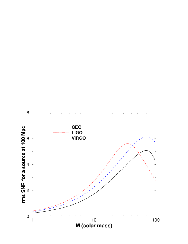
Figure 17: Signal-to-noise ratio, in initial interferometers, as a function of total mass, for inspiral signals from binaries of equal masses at 100 Mpc and averaged over source inclination and location. (TAMA has been left out as the SNRs in that case are too low for these sources.)

For intermediate mass black hole binaries of mass in the range of 100 solar masses, VIRGO and GEO can achieve excellent SNRs. There is no convincing evidence for the existence of BHs of such masses, and their binaries, but future GW observations should shed light on these systems.

As mentioned earlier, enhanced interferometers will have ten times better sensitivity and bandwidth and will therefore be able to achieve similar SNRs at 1 Gpc. As we have seen in earlier Sections at such distances the event rate builds up to several per week. Construction of these advanced interferometers will, therefore, make routine detection of compact binary inspirals and coalescences possible and thereby open up the new gravitational window for observation.

The SNRs achievable for the LISA detector is phenomenal and is listed in Table 7. LISA should be able to observe $\sim$ million solar mass BH inspiral almost anywhere in the Universe. The time spent by a binary in the LISA band width can be larger than the life time of the detector. For this reason we have expressed the SNR in the above equation in terms of the frequency range $(f_{1},f_{2})$ in which the signal is extracted during a given observational period. For a given duration of observation the binary signal will be the strongest if the observation starts closest to the instant of coalescence and therefore we shall take $f_{2}=f_{\rm LSO}.$

Table 7: Signal-to-noise ratios in LISA for supermassive binary black holes and stellar mass compact objects falling into them, at a cosmological distance of 3 Gpc.

$m_{1}(M_{\odot})$	$m_{2}(M_{\odot})$	$f_{1}$ (Hz)	$f_{\rm lso}$ (Hz)	$\rho$
$10^{7}$	$10^{7}$	$1.08\times 10^{-5}$	$2.2\times 10^{-4}$	$1900$
$10^{6}$	$10^{6}$	$4.54\times 10^{-5}$	$2.2\times 10^{-3}$	$4900$
$10^{5}$	$10^{5}$	$1.92\times 10^{-4}$	$2.2\times 10^{-2}$	$1700$
$10^{6}$	$10$	$2.75\times 10^{-3}$	$4.4\times 10^{-3}$	$21$
$10^{5}$	$10$	$5.55\times 10^{-3}$	$4.4\times 10^{-2}$	$11$
$10^{6}$	$1.4$	$3.93\times 10^{-3}$	$4.4\times 10^{-3}$	$3.8$
$10^{5}$	$1.4$	$1.15\times 10^{-2}$	$4.4\times 10^{-2}$	$2.2$

8.3 Sensitivity to stochastic gravitational waves

In Secs. 5 and 6 we have seen how astrophysical processes can generate a stochastic background of GW and what physical interactions can produce a background in the early Universe, respectively. A stochastic background is easily detected if the instrumental and environmental background noise levels in a detector are much smaller than the GW background and especially if the statistical properties of the GW background or its spectral characteristics, are different from what is expected for the background noise.

Even when the GW background is far too small compared to the instrumental noise backgrounds, the theory of matched filtering developed in the previous Sections, for the detection of deterministic signals, can be generalised to the case of a stochastic background of gravitational radiation. As opposed to deterministic signals we will not have the advantage of using a template that we can compute before hand. Rather, the idea is to use the (noisy) data in one detector, in which a stochastic background may be present, as a template to detect the background in (noisy) data from another detector. In other words, we can use the ‘noisy template’ from one detector to match filter the background in another. Because our template is noisy, the enhancement in SNR will not be as good as in the case of matched filtering a deterministic signal. However, as the background will always be present, if we can correlate the outputs of two detectors for a long enough duration, in principle, the background will show up above other noise sources.

The idea that one detector output can be used as a template to enhance the visibility of the background in another essentially assumes that (1) the two detectors record identical GW signals and (2) the instrumental noise in the two detectors are uncorrelated. In reality neither of these assumptions will hold good perfectly. If a pair of detectors happen to be close together on Earth, so that they record identical stochastic signals, then they will also be affected by similar environmental disturbances such as seismic activity, wind, storm, etc., so that the background noise might have a large non-GW correlation. If the two detectors are far apart then their environmental disturbances are unlikely to be correlated but they may be registering different polarisations and phases of the background GW so that the cross-correlation might be insignificant. Clearly, a compromise is in order: Two widely separated detectors are good for cancellation of the noise background, while two nearby detectors are favoured for enhancing the signal background. In what follows we will derive the SNR enhancement achieved on cross-correlating data from two identical detectors placed at the same location. The following derivation is a heuristic one to indicate how the cross-correlation works; see Ref. [159, 160] for a more rigorous derivation involving two detectors of different orientations.

Let $x_{1}(t)$ and $x_{2}(t)$ denote the outputs of two interferometric antennas located nearby to each other and having the same orientation. They will both have the same stochastic signal $h(t)$ and we will assume that the internal noises $n_{1}(t)$ and $n_{2}(t)$ are uncorrelated. We will also assume that the rms value of the internal noise is much larger than the rms value of the stochastic signal we wish to detect. Thus, we can write

$$x_{1}(t)=n_{1}(t)+h(t),\ \ \ \ x_{2}(t)=n_{2}(t)+h(t),\ \ \ \ \overline{n_{1}^{2}}=\overline{n_{2}^{2}}\gg\overline{h^{2}},$$ (137)

where an overline indicates the ensemble average and we have assumed that the ensemble averages of the background noise and stochastic signal are both zero. In order to extract the stochastic background we construct the cross-correlation integral $C.$ The cross-correlation of the two detector outputs each lasting a time $T$ is given by

$$C^{2}\equiv\int_{-T/2}^{T/2}x_{1}(t)x_{2}(t)dt\equiv\left(x_{1},x_{2}\right),$$ (138)

where we have introduced the bracket notation to denote the cross-correlation of two data sets $x_{1}$ and $x_{2}.$ The cross-correlation is denoted as $C^{2}$ since it is quadratic in the useful signal $h.$ Using Eq. (137) $C^{2}$ can be written as

$$C^{2}=\left(n_{1},n_{2}\right)+\left(n_{1},h\right)+\left(h,n_{2}\right)+\left(h,h\right).$$ (139)

$C^{2}$ is a random process whose average, under the assumption that the internal detector noises are uncorrelated, gives the useful signal $S^{2}$

$$S^{2}=\overline{C^{2}}=\overline{\left(h,h\right)}.$$ (140)

From the above equation we conclude that the signal component of $C^{2}$ grows in proportion to the integration time $T,$ i.e., $S^{2}\propto T.$ This, of course, is only the statistical average of $C^{2}$ and it must be compared with the fluctuation in $C^{2}$ to deduce its significance. Let us define the noise component of $C^{2}$ by

$$N^{2}\equiv C^{2}-\overline{C^{2}}=\left(n_{1},n_{2}\right).$$ (141)

$N^{2}$ is also a random variable and its rms value will involve the noise spectral densities [cf. Eqs. (98) and (100)] $S_{n_{1}}(f)$ and $S_{n_{2}}(f)$ of the two detectors. Assuming that the two detectors have identical noise spectra, say $S_{n}(f)$, the rms value of $N^{2}$ turns out to be

$$\overline{N^{4}}\propto T\int_{-\infty}^{\infty}dfS_{n}^{2}(f).$$ (142)

We see from Eqs.(140) and (142) that the SNR for the stochastic background grows as $S/N\propto T^{1/4}.$ Therefore, in principle, a stochastic background that is below the internal noise can be extracted by integrating for a sufficiently long duration. Conversely, given that we have data sets of a certain duration $T$ with internal noise spectrum $S_{n}(f),$ we can estimate the minimum level of the stochastic background we can extract. These estimates show that initial interferometers will be able to detect a stochastic background at the level of $h(f)\approx 2\times 10^{-23}$, or $\Omega_{\rm GW}\sim 5\times 10^{-6},$ (cf. Sec.6), with a 90 % confidence level, after three months of integration [160]. Advanced ground-based detectors should be able to reach a level that is five orders of magnitude lower (in terms of $\Omega_{\rm GW}$). The space-based LISA will have sensitivity to primordial background similar to the advanced ground-based detectors but in a frequency range $\sim 10^{-4}$-$10^{-1}$Hz where the primordial background has larger spectral amplitudes $h(f)$. Since LISA is likely to be in place around the same time as the third generation advanced ground-based detectors, there is an exciting possibility to detect primordial background, of the kind discussed in Sec. 6, within the next decade. They will also help us to understand populations of astrophysical sources that generate a stochastic GW background of the sort discussed in Sec. 5.

8.4 Computational Costs

Matched filtering places stringent demands on the knowledge of the signal’s phase evolution which depends on two things: (1) our modeling of the signal and (2) the parameters characterising the signal. If our signal model is inaccurate or if the signal’s parameters are unknown, there could be a loss in the SNR extracted. For instance, in the case of inspiral signals, a mismatch of one cycle in $10^{4}$ cycles leads to a drop in the SNR by more than a factor of two, losing a factor of eight in the number of potentially detectable events. (Recall that the SNR is inversely proportional to the distance to a source; thus an SNR loss by a factor $a$ will reduce the span of a detector by the same factor, resulting in a decrease in the volume of observation, and hence the number of events, by a factor $a^{3}.$) Moreover, since the parameters of a signal will not be known in advance, it is necessary to filter the data with a family of templates located at various points in the parameter space—e.g., placed on a lattice—such that any signal will lie close enough to at least one of the templates to have a good cross-correlation with that template. The number of such templates is typically very large. This places a great demand on the computational resources needed to make an on-line search, that is to search for signals in the detector output at the same rate at which data is acquired. We shall discuss below the method of finding the number of templates to filter any known signal and the computational resources required to analyse the data on-line. In the next Section we will discuss the tools needed in parameter estimation.

8.4.1 Ambiguity function

Ambiguity function, well known in statistical theory of signal detection [167], is a very powerful tool in signal analysis: It helps in making estimates of variances and covariances involved in the measurement of various parameters, in computing biases introduced in using a family of templates whose shape is not the same as that of a family of signals intended to be detected, in assessing the number of templates required to span the parameter space of the signal, etc. We discuss parameter estimation in this Section and computational costs in the next.

We begin by defining a normalised waveform. A waveform $a$ is said to be normalised if it has unit norm: $||a||\equiv\left<a,a\right>^{1/2}=1.$ The norm $h_{0}$ of a signal $h$ is also its optimal SNR: $\rho_{\rm opt}=\left<h,h\right>^{1/2}=||h||=h_{0}.$ For this reason the norm of a signal is also referred to as the signal strength.

The ambiguity function is defined as the scalar product of two normalised waveforms maximised over the initial phase of one of the waveforms. More precisely, it is the absolute value of the scalar product of two normalised waveforms.

Let $a(t;{\alpha})$ be a normalised waveform. Note that we use the symbol $a$ to denote a family of waveforms all having the same functional form but differing from one another in the parameter values. Indeed, ${\alpha}=\{\alpha^{A}|A=0,\ldots,p\}$ denotes the parameter vector comprising of $p+1$ parameters. It is conventional to choose the parameter $\alpha^{0}$ to be the lag $t^{\prime},$ which simply corresponds to a coordinate time when an event occurs and is, therefore, called an extrinsic parameter, while the rest of the $p$ parameters, $\alpha^{k},\ k=1,\ldots,p,$ are called the intrinsic parameters and characterise the GW source. Given two normalised waveforms, $a(t;{\alpha_{1}})$ and $a(t;{\alpha_{2}}),$ whose parameter vectors are not necessarily the same, the ambiguity ${\cal A}$ is defined as

$${\cal A}({\alpha_{1}},{\alpha_{2}})\equiv\max_{\alpha^{0}}\left|\left<a({\alpha_{1}}),a({\alpha_{2}})\right>\right|.$$ (143)

Since the waveforms are normalised it follows that ${\cal A}({\alpha_{1}},{\alpha_{1}})=1,$ and, if $\alpha_{1}$ is not equal to $\alpha_{2},$ ${\cal A}({\alpha_{1}},{\alpha_{2}})\leq 1.$

It is important to note that in the definition of the ambiguity function there is no need for the functional forms of the template and signal to be the same; the definition holds good for any signal-template pair of waveforms. Moreover, the number of template parameters need not be identical (and usually aren’t) to the number of parameters characterising the signal. For instance, a binary can be characterised by a large number of parameters, such as the masses, spins, eccentricity of the orbit, etc., while we may take as a model waveform the one involving only the masses. In the context of inspiral waves $a(t;{\alpha_{2}})$ is the exact general relativistic waveform emitted by a binary, whose form we do not know, while the template family is a post-Newtonian, or some other, approximation to it, that will be used in detecting the true waveform. Another example would be signals emitted by spinning neutron stars, isolated or in binaries, whose time evolution is unknown, either because we cannot anticipate all the physical effects that affect their spin, or because the parameter space is so large that we cannot possibly take into account all of them in a realistic search. Of course, in such cases we cannot compute the ambiguity function since one of the arguments to the ambiguity function would be unknown. These are indeed issues where substantial work is called for. For this Review it suffices to assume that the signal and template wave forms are of identical shape and the number of parameters in the two cases is the same.

In the definition of the ambiguity function Eq. (143) ${\alpha_{1}}$ can be thought of as the parameters of a (normalised) template, while ${\alpha_{2}}$ those of a signal. With the template parameters ${\alpha_{1}}$ fixed, the ambiguity function is a function of $p$ signal parameters $\alpha^{k}_{2},\ k=1,\ldots,p,$ giving the SNR obtained by the template for different signals. However, one can equally well interpret the ambiguity function as the SNR obtained for a given signal by filters of different parameter values. Now, the region in the signal parameter space for which a template obtains SNRs larger than a chosen value, called the minimal match [179], is the span of that template. Templates should be chosen so that together they span the entire signal parameter space of interest with the least overlap of one other’s spans.

8.4.2 Metric on the space of waveforms

The computational costs of our searches and the estimation of parameters of a signal, afford a lucid geometrical picture [180, 179]. To develop this picture we begin with the space of signal waveforms. A waveform $e(t;{\alpha}),$ with a given set of values of its parameters, can be thought of as a unit vector. (In much of the discussion below we will deal with unit signal and template vectors.) The set of sample values $h=\{h_{k}|k=0,\ldots,N-1\}$ of a waveform, sampled at times $t_{k},$ $k=0,\ldots,N-1,$ can be thought of as an $N$-dimensional signal vector but not necessarily of unit norm. Indeed, the output of a detector sampled in the same way can also be regarded as an $N$-dimensional vector. The set of all detector output vectors forms a vector space. Returning to the signal vector, as its parameters are varied the signal vector spans a space in the underlying N-dimensional vector space of detector outputs. The dimension of this sub-space is equal to the number of parameters of the signal and is called the signal space.

The signal space, which is a sub-space of the full vector space, has a manifold structure, the parameters of the wave constituting a coordinate system and the dimensionality of the space being equal to the number of parameters. Having defined a manifold we can ask if it is possible to define a meaningful metric on this manifold. Indeed, we already have the necessary tool to define the metric, namely the ambiguity function.

Let us fix the template parameters $\alpha_{1}$ of the template in which case the ambiguity function is a function of $p+1$ signal parameters $\alpha_{2}^{k},$ $k=0,\ldots,p.$ Expanding ${\cal A}(\alpha_{1},\alpha_{2})$ about its maximum $\alpha_{2}=\alpha_{1}$ and retaining only quadratic terms we get:

$${\cal A}({\alpha_{1}},{\alpha_{2}})=1-\gamma_{AB}\Delta\alpha^{A}\Delta\alpha^{B}+O[(\Delta{\alpha})^{3}],$$ (144)

where $\Delta{\alpha}\equiv{\alpha_{2}}-{\alpha_{1}}$ and $\gamma_{AB}$ is the metric on the space of waveforms:

$$\gamma_{AB}({\alpha_{1}})\equiv-\frac{1}{2}\left.\frac{\partial^{2}{\cal A}({\alpha_{1}},{\alpha_{2}})}{\partial\alpha_{2}^{A}\partial\alpha_{2}^{B}}\right|{\atop\scriptstyle\alpha_{2}=\alpha_{1}}.$$ (145)

This is the metric at the point $\alpha_{1}$ on the manifold. From now on we shall drop the suffix $1$ on the parameter $\alpha$ since it really represents an arbitrary point on the manifold where a template resides. Since one can easily maximise over the lag parameter $\alpha^{0}$ it is desirable to work with the metric $g_{ij}$that is projected orthogonal to $\alpha^{0},$ namely

$$g_{ij}\equiv\gamma_{ij}-\frac{\gamma_{i0}\gamma_{j0}}{\gamma{ij}}\ \ \ \ i,j=1,\ldots,p.$$ (146)

Let us suppose that it is required to make a choice of a template bank. By a template bank we mean a discrete family of signal waveforms chosen in a given region of the signal parameter space. In such a template bank no template waveform will perfectly match an incoming signal but if the density of templates is large enough then it may be possible to extract every signal with an SNR larger than a certain fraction of the optimal SNR. Most of the early GW data analysis literature concerned itself in studying efficient algorithms to set up a template bank so as to minimise the computational costs of a search. The density of templates in the bank depends on what is the largest fraction of the optimal SNR one is prepared to lose in a search: Smaller this fraction greater is the density of templates. One is normally interested in setting up a bank such that each possible signal will have its maximised overlap larger than a certain minimal match $(MM)$ with at least some member of the bank. By overlap we mean the scalar product of a (normalised) signal waveform with a (normalised) template waveform and maximisation is over all the template parameters. The maximised overlap, sometimes referred to as the match, is always smaller than or equal to one. Demanding that the proper distance between templates, namely $g_{ij}\Delta\alpha^{i}\Delta\alpha^{j}$ be as large as possible, for a given minimal match $MM,$ we can obtain the following formula for a spacing of templates using Eq. (144):

$$\Delta\alpha^{k}=\sqrt{\frac{2(1-MM)}{g_{kk}}}$$ (147)

where a factor 2 in the numerator arises because a proper distance of $(1-MM)$ between the least matched signal and a template implies that the proper distance between templates be twice that value, assuming that the templates are placed on a square lattice.

The distance between templates can also be computed more precisely by employing numerical methods, as was done in [175] (also see [181]). A comparison of the metric-based method discussed above and the numerical method shows that the quadratic approximation (147) is good typically for ${\cal A}\geq 0.95$. Thus, in the limit of close template spacing, Eq. (147) can be used to make a choice of templates.

We now turn our attention to the use of the metric in calculating the number of templates needed for a search. If the number ${\cal N}$ of templates needed to cover a region of interest is large, ${\cal N}$ is well approximated by dividing the proper volume of the region of interest on the signal manifold space by the proper volume per template. The proper volume per template, $\Delta V$, depends on the packing algorithm used, which in turn depends on $p$ the dimension of the parameter space. For instance, we used a square lattice above. For $p=2$, the optimal packing is a hexagonal lattice, and thus

$$\Delta V=\frac{3\sqrt{3}}{2}(1-MM).$$ (148)

There is no packing scheme which is optimal for all $p$, but it is always possible (though inefficient) to use a hypercubic lattice, for which

$$\Delta V=(2\sqrt{(1-MM)/p})^{p},$$ (149)

as a starting point. Once the span of a template is known the total number of templates is straightforward to compute using

$${\cal N}=\frac{\int d^{p}{\alpha}\,\sqrt{\det\|g_{ij}\|}}{\Delta V},$$ (150)

where $p$ is, as before, the dimension of the parameter space.

8.4.3 Computational costs for binary inspiral search

The number of templates for binary inspiral searches has been computed for the post-Newtonian signals and ground-based interferometers discussed earlier [181]. The numbers required at a high minimal match $MM=0.97$ are several hundreds of thousands (cf. Table 8) and imply huge computational costs. For instance, to search for inspiral waves on-line (i.e. to search at the same rate as the rate at which data is recorded) we would require a dedicated computer that can carry out $10^{10}$ floating point operations per second (i.e., 10 GFLOPS). Building economical computers of such speed is the prime concern of various data analysis groups at the moment.

Table 8: Number of templates required to search for inspiral waves from a binary consisting of stars of mass $m_{1},m_{2}\geq 0.2M_{\odot}$ and minimal match of 0.97. The numbers are given for different post-Newtonian families of waveforms.

Interferometer	1PN	1.5PN	2PN
LIGO-I	$2.5\times 10^{5}$	$5.3\times 10^{5}$	$4.7\times 10^{5}$
VIRGO	$1.4\times 10^{7}$	$1.4\times 10^{7}$	$1.3\times 10^{7}$
GEO600	$4.3\times 10^{5}$	$8.5\times 10^{5}$	$7.5\times 10^{5}$

8.4.4 Computational costs to search for continuous waves

The search problem for continuous waves from spinning neutron stars is the most compute-intensive job in gravitational wave data analysis. Today, there is little hope that all-sky searches lasting for a year or more, can be made. It is easy to see why this is such an intensive job: Firstly, the data has to be collected continuously for months together and at a good sensitivity. No one has run interferometers for periods as long as that and we do not yet know if this would be possible. Secondly, though a neutron star emits a periodic signal in its rest frame, save for the neutron star spin-down which indeed induces some modulation in the waveform, because of Earth’s acceleration relative to the source, the detector does not see a periodic wave. The wave is both frequency- and amplitude-modulated. One can, fortunately, de-modulate these effects since Earth’s motion is known quite accurately, and hence recover the original periodic signal. But de-modulation requires a knowledge of the source’s direction and its frequency, which are unknown in a blind search. The angular resolution one obtains in a year’s integration is $\Delta\theta=\lambda/D,$ where $\lambda$ is the wave length of radiation and $D$ is the baseline of the detector in a year’s integration, namely 1 A.U. Thus, for $f=100$ Hz we have $\Delta\theta=10^{-5}$ rad or about two arcsec. Now, assuming that the source may be in any one of the 4 arcsec² patches on the sky we get the number of patches in the sky for which we will have to try out a de-modulation correction to be $4\pi/(\Delta\theta)^{2}=4\pi 10^{10}.$ It is quite an impossible task to apply Doppler de-modulation to the detector output for each of these $\sim 10^{11}$ patches and compute as many Fourier transforms.

One, therefore, asks the question given a compute power what is the best possible search one can do? Is there any advantage in going from a one-step search to a two- or multi-step hierarchical search? What about directional searches? These are some of the problems for which we have some answer; but a great deal of work is needed and is currently under progress, to improve and optimise search algorithms. In the following we will provide a summary of the current status.

The differential geometric formalism discussed above has been used [182] to compute the number of days of data that a TFLOPS-class computer can analyse on-line (that is, analyse $T$-hours of data in $T$ hours) and carry out a blind (that is, unknown direction, frequency and spin-down rate) search. Unfortunately, the longest data we can integrate on-line, for neutron stars with spin frequencies $f\leq 100$ Hz and spin-down rates less than 1000 years, is about 18 days. This yields a SNR lower by a factor of 5 as compared to a year’s worth of observing. On-line searches for neutron stars with $f\leq 500$ Hz (largest observed frequencies of millisecond pulsars) and spin-down rates of 40 years (shortest observed spin-down rates), can only be made for a data set lasting for a duration of 20 hours or less. If the source’s position is known in advance, but not its frequency, then one can carry out an on-line search, again with a TFLOPS-class computer, for the frequency of the source in a data set that is worth 3 months long. This is good news since there are many known pulsars and X-ray binary systems that are potential sources of radiation. In addition, the obvious targeted search locations are the centre of the Galaxy and globular clusters.

There have been efforts [183, 184] to study the effectualness of a two-step hierarchical method for a blind search. Here the basic idea is to construct Fourier transforms of data sets of duration smaller than the period in which Doppler modulations will be important and to stack spectral densities obtained in this way and to add them all up. This is an incoherent way of building the signal since one adds spectral densities that have no phase information. Therefore, one gains in SNR less than what an optimal matched filtering method is able to achieve. However, this does not matter since (i) the targeted SNR’s are quite high $\sim 10$ and (ii) candidate events can always be followed-up using coherent integration methods. These methods afford an on-line all-sky blind search (i.e., a search in which no assumptions are made about the parameters of the source) for continuous gravitational waves for a period of 4 months or less using a 20 GFLOPS computer. Detector groups are planning to build computers of this kind to aid in their search for continuous GW.

8.5 Covariance Matrix and Parameter Estimation

After a detection has been made, say because a high SNR has been recorded that could not be vetoed out, the next step in data analysis is estimation of parameters characterising the event and provide error bounds on the measured values. The first thing to note is that one can never be absolutely certain that a signal is present in a data train; one can only give confidence levels about its presence which could be close to 100% at high values of the SNR. Confidence level is a measure of the probability that the observation of an event, such as a large peak in the correlated output, is generated by a gravitational wave signal as opposed to a random, non-gravitational wave process. The next thing to note is that howsoever high the SNR may be one can’t be absolutely certain about the true parameters of the signal: At best one can compute a range of values in which the true parameters of the signal are most likely to lie. The width of the range depends on the confidence level demanded, being larger for higher confidence levels.

In our search for a signal in the output of a detector we use a discrete, rather than a continuous, family of templates. Each template has a particular set of values of the parameters and the templates together span an interesting region of the parameter space. The spacing between templates in the parameter space will, in general, be quite small. A common estimate of the signal parameters is given by the parameters of the template that obtains the maximum SNR. Such an estimate is called the maximum likelihood estimate – so-named because the parameters of this template maximise what is called the likelihood ratio [167]. Maximum likelihood estimates are not always the minimum uncertainty estimates, as has been particularly demonstrated for the case of binary inspiral signals [180]. Bayesian estimates, which take into account any prior knowledge that may be available about the distribution of the source parameters, as well as the knowledge from the output of a whole bank of templates rather than a single template, often give a much better estimate [185]. The reason for the better performance of Bayesian estimates is that they make a quantitative use of the information at hand.

In a measurement process any estimation of parameters, howsoever efficient, robust and accurate, is unlikely to give the actual parameters of the signal since, at any finite SNR, the presence of noise alters the input signal. In geometric terms, the signal vector is being altered by the noise vector resulting in a vector that lies outside the signal manifold. Techniques such as matched filtering aim at computing the best projection of this altered vector onto the signal space. The true parameters of the signal are expected to lie within an ellipsoid of $p$ dimensions at a certain level of confidence – the volume of the ellipsoid increasing with the level of confidence. The axes of the ellipsoid are the 1–$\sigma$ uncertainties in the estimation of parameters and the confidence level corresponding to a 1–$\sigma$ uncertainty is $0.67^{p}$, confidence level corresponding to a 2–$\sigma$ uncertainty is $0.95^{p},$ and so on.

The topic of parameter estimation deserves a much wider discussion than given here. However, our goal here is only to assemble the necessary tools from estimation theory for ready use. Interested reader can consult the ever-growing literature for further details. (See, Ref. [167] for estimation theory and [180, 186, 187, 188] for applications in GW observations.)

8.5.1 Covariance matrix

The scalar product Eq. (113) induces the following metric on the signal manifold [180]:

$$G_{ij}=\left<{\partial a({\alpha})\over\partial\alpha^{i}},{\partial a({\alpha})\over\partial\alpha^{j}}\right>,$$ (151)

where $a(\alpha)$ is a signal vector of unit norm and $\alpha^{i}$ are the coordinates. The metric $G_{ij}$ is defined on the manifold of all the parameters including the lag $t^{\prime}$ and the initial phase $\phi_{0}$ of the waveform. It is easy to show that $G$ projected orthogonal to the initial phase $\phi_{0}$ yields the metric $\gamma$ in Eq.(145).

The metric on the space of waveforms introduced above is also called the Fisher information matrix [167]. Indeed, it contains the ‘information’ about how similar or dissimilar are the waveforms in a small neighbourhood around the parameter $\alpha$ of the signal. Large values of the metric imply that even small changes in signal and template parameters can greatly affect their overlap while the opposite is true when the metric coefficients are small.

The inverse of the information matrix is the covariance matrix $C_{ij},$ whose diagonal and off-diagonal elements are, in the limit of large SNR, the variances in the measured values of the parameters and correlation coefficients among different parameters, respectively [167]:

$$C_{ij}=\left(G\right)^{-1}_{ij}.$$ (152)

Covariance matrix based errors in the estimation of the total mass, reduced mass and the instant of coalescence $t_{C}$ have been computed by Poisson & Will [188] for the second post-Newtonian inspiral waveforms. They are listed in Table 9 for three archetypal binaries. The relative errors are smaller, for a given SNR, in the case of lighter binaries. This is because lighter binaries last for a longer duration and have a larger number of cycles in the detector, making it relatively easier, as compared to higher mass binaries, to discriminate waveforms of different parameters.

Table 9: Errors in the estimation of instant of coalescence $\Delta t_{C},$ phase at coalescence $\Delta\phi_{C},$ chirp mass $\Delta{\cal M}/{\cal M},$ and symmetric mass ratio $\Delta\eta/\eta,$ and percentage bias in the estimation of the total mass ${\cal B}_{m}=100(1-m^{T}/m^{X})$ and percentage bias in the estimation of the mass ratio ${\cal B}_{\eta}=100(1-\eta^{T}/\eta^{X}),$ where $T$ stands for the parameter of the template and $X$ for the parameter of exact wave form, for the second-post-Newtonian corrected inspiral waveform neglecting the effect of spins. Values are quoted for three archetypal binaries consisting of two 1.4 $M_{\odot}$ NSs (system NS-NS), a 1.4 $M_{\odot}$ NS and a 10 $M_{\odot}$ black hole (system NS-BH), and two 10 $M_{\odot}$ black holes (system BH-BH).

System	$\Delta t_{C}$ (ms)	$\Delta\phi_{C}$ (rad)	$\Delta{\cal M}/{\cal M}$ ($10^{-3}$)	$\Delta\eta/\eta$	${\cal B}^{T}_{m}$	${\cal B}^{T}_{\eta}$
NS-NS	1.07	2.94	0.36	0.28	$0.214$	$0.211$
NS-BH	1.72	2.27	2.20	0.50	$-6.96$	$12.2$
BH-BH	1.50	2.19	5.40	1.50	$1.40$	$0.282$

8.5.2 Biases in estimation

There are two ways in which an error can occur in the estimation of signal parameters. Firstly, an error in the measurement of a parameter occurs because of internal noise which alters the input signal and hence, in the process of maximising the SNR, we err in the estimation of parameter by an amount that depends on the SNR. This type of error is a random error and normally goes down in inverse proportion to the SNR. In the limit of an infinitely large ensemble of measurements the estimated values converge to the true values of the signal parameters. Secondly, our estimator may be a biased estimator in the sense that the average over an ensemble of measurements might converge to values different from the true values of the parameters. This can happen because of one or both of the following two reasons: The search templates we use in our detection algorithms might only be an approximation to the true signal, as in the case of inspiral wave searches where we use post-Newtonian search templates to look for the fully general relativistic signal. As we shall show below, such a search would induce a bias in the estimation of parameters, which we shall refer to as the bias of the first kind. Alternatively, the estimator might be inherently a biased estimator and may give erroneous values even if the search templates are not faulty which we shall refer to as the bias of the second kind.

An example of the bias of the second kind is the following. In the maximum likelihood method we always aim for the largest value of the likelihood ratio. This has the effect of making a higher estimation of the amplitude parameter of the signal as shown in [180]. For inspiral signals, this would mean that the distance to the source would be under-estimated.

Biases in parameter estimation for inspiral signals have been discussed in [189]. Biases in the estimation of the total mass and the symmetric mass ratio on using standard post-Newtonian approximation are quoted in Table 9 and discussed in detail in [170]. They find that while using standard post-Newtonian approximation to the waveform the bias could be quite large, whereas $P$–approximants to inspiral waves greatly reduce the bias in the estimation of parameters.

8.6 Conclusions

Gravitational waves in ground-based interferometers are expected to be below the noise levels of first and second generation instruments. We have seen in this Section how a prior knowledge of the signal’s shape can be used in enhancing the visibility of the signal. With the aid of matched filtering a network of initial interferometers, consisting of GEO, LIGO and VIRGO, should be able to survey a volume of $3\times 10^{6}$ Mpc³ for binary black holes at a minimum SNR of 3. In this volume conservative estimates of coalescence rates predict about a few per year. Thus, the binary black holes may be the first events to be registered in our detectors.

Initial interferometers should also be able detect primordial gravitational wave background at the level of $\Omega_{\rm GW}\sim 5\times 10^{-6}$ by cross-correlating data in nearby interferometer pairs (LIGO-LIGO or GEO-VIRGO). However, this is at a level rather too small from a theoretical point of view. New data analysis algorithms that exploit the specific signature of the primordial background may aid in detecting the background at a much lower level but, at the moment, we do not know how to achieve this.

Initial interferometers will also be able to detect continuous gravitational waves from newly born or rapidly spinning non-spherical neutron stars provided that the amplitude is $h\geq 10^{-26}$ and the signal lasts for a few months. This, of course, assumes that we know the evolution of the phase of the signals emitted in the process which, for old neutron stars is a simple sinusoid. However, in the case of waves emitted due to one of the instabilities we do not have the right templates. This is also true of transient waves emitted during a supernova explosion or the merger of black holes. Thus, much work is needed in understanding sources of gravitational waves. Indeed, it may very well be that the new generation of gravitational wave antennas will open up a new window for observing the Universe which will aid in our understanding of strong and non-linear gravity.

Acknowlegements

We appreciate useful discussions with K. Thorne, V. Braginsky, and B. Schutz. This work was supported in part by a joint research grant from the Royal Society.

1 Appendix

Here we summarize some basic formulae relevant for the description of massive binary evolution.

A1 Keplerian binary system and radiation back reaction

Binary stars is one of the main topics of the present paper, so it is necessary to remind the reader some basic facts about Keplerian motion in a binary system. The stars are highly concentrated objects, so their treatment as point masses is usually adequate for the description of their interaction in the binary. Further, the Newtonian gravitation theory is sufficient for this purpose as long as the orbital velocities are small in comparison with the speed of light $c$. The systematic change of the orbit caused by the emission of gravitational waves will be considered in a separate paragraph below.

A1.1 Keplerian motion

Let us consider two point masses $M_{1}$ and $M_{2}$ orbiting each other under the force of gravity. It is well known (see [190]) that this problem is equivalent to the problem of a single body with mass $\mu$ moving in an external gravitational potential. The value of the external potential is determined by the total mass $M$. The total mass $M$ of the system is

$$M=M_{1}+M_{2}\,,$$ (A1)

and the reduced mass $\mu$ is

$$\mu=\frac{M_{1}M_{2}}{M}\,.$$ (A2)

The body $\mu$ moves along an elliptic orbit with eccentricity $e$ and major semiaxis $a$. The orbital period $P$ and orbital frequency $\Omega=2\pi/P$ are related with $M$ and $a$ by the 3d Kepler’s law

$$\Omega^{2}=\left(\frac{2\pi}{P}\right)^{2}=\frac{GM}{a^{3}}\,.$$ (A3)

This relationship is true for any eccentricity $e$.

Individual bodies $M_{1}$ and $M_{2}$ move around the barycentre of the system in elliptic orbits with the same eccentricity $e$. Major semiaxes $a_{i}$ of the two ellipses are inversely proportional to the masses:

$$\frac{a_{1}}{a_{2}}=\frac{M_{2}}{M_{1}}\,$$ (A4)

and satisfy the relationship $a=a_{1}+a_{2}$. The position vectors of the bodies from the system’s barycenter are ${\mathbf{r}}_{1}=M_{2}{\mathbf{r}}/(M_{1}+M_{2})$ and ${\mathbf{r}}_{2}=-M_{1}{\mathbf{r}}/(M_{1}+M_{2})$, where ${\mathbf{r}}={\mathbf{r}}_{1}-{\mathbf{r}}_{2}$ is the relative position vector. Therefore, the velocities of the bodies with respect to the system’s barycentre are related by

$$-\frac{{\mathbf{V}}_{1}}{{\mathbf{V}}_{2}}=\frac{M_{2}}{M_{1}}\,,$$ (A5)

and the relative velocity is ${\mathbf{V}}={\mathbf{V}}_{1}-{\mathbf{V}}_{2}$.

The total conserved energy of the binary system is

$$E=\frac{M_{1}{\mathbf{V_{1}}}^{2}}{2}+\frac{M_{2}{\mathbf{V_{2}}}^{2}}{2}-\frac{GM_{1}M_{2}}{r}=\frac{\mu{\mathbf{V}}^{2}}{2}-\frac{GM_{1}M_{2}}{r}=-\frac{GM_{1}M_{2}}{2a}\,$$ (A6)

where $r$ is the distance between the bodies. The orbital angular momentum vector is perpendicular to the orbital plane and can be written as

$${\mathbf{J_{orb}}}=M_{1}{\mathbf{V}}_{1}\times{\mathbf{r}}_{1}+M_{2}{\mathbf{V}}_{2}\times{\mathbf{r}}_{2}=\mu{\mathbf{V}}\times{\mathbf{r}}.$$ (A7)

The absolute value of the orbital angular momentum is

$$|{\mathbf{J_{orb}}}|=\mu\sqrt{GMa(1-e^{2})\,}.$$ (A8)

For circular binaries with $e=0$ the distance between orbiting bodies does not depend on time

$$r(t,e=0)=a$$

and is usually referred to as orbital separation. In this case, velocities of the bodies, as well as their relative velocity, are also time-independent:

$$V\equiv|{\mathbf{V}}|=\Omega a=\sqrt{GM/a}\,,$$ (A9)

and the orbital angular momentum becomes

$$|{\mathbf{J}}_{orb}|=\mu Va=\mu\Omega a^{2}.$$ (A10)

A1.2 Gravitational radiation from a binary

The plane of the orbit is determined by the orbital angular momentum vector ${\mathbf{J}}_{orb}$. The line of sight is defined by a unit vector ${\mathbf{n}}$. The binary inclination angle $i$ is defined by the relation $\cos i=({\mathbf{n}},{\mathbf{J}}_{orb}/J_{orb})$ such that $i=90^{\circ}$ corresponds to the system visible edge-on.

Let us start from two point masses $M_{1}$ and $M_{2}$ in a circular orbit. In the quadrupole approximation [2], the two polarization amplitudes of GW at a distance $r$ from the source are given by

$$h_{+}=\frac{G^{5/3}}{c^{4}}\frac{1}{r}\,2(1+\cos^{2}i)(\pi fM)^{2/3}\mu\cos(2\pi ft)$$ (A11)

$$h_{\times}=\pm\frac{G^{5/3}}{c^{4}}\frac{1}{r}\,4\cos i(\pi fM)^{2/3}\mu\sin(2\pi ft)$$ (A12)

Here $M$ is the total mass, $\mu$ is the reduced mass, and $f=\Omega/\pi$ is frequency of the emitted GW (twice the orbital frequency). Note that for a fixed distance $r$ and a given frequency $f$, the GW amplitudes are fully determined by $\mu M^{2/3}={{\cal M}}^{5/3}$, where the combination

$${\cal M}\equiv\mu^{3/5}M^{2/5}$$

is called the “chirp mass” of the binary. After averaging over orbital period (so that the squares of periodic functions are replaced by 1/2) and orientations of binary orbital plane, one arrives at the averaged (characteristic) GW amplitude

$$h(f,{\cal M},r)=(\langle h_{+}^{2}\rangle+\langle h_{\times}^{2}\rangle)^{1/2}=\left(\frac{32}{5}\right)^{1/2}\frac{G^{5/3}}{c^{4}}\frac{{\cal M}^{5/3}}{r}(\pi f)^{2/3}$$ (A13)

A1.3 Energy and angular momentum loss

In the approximation and under the choice of coordinates that we are working with, it is sufficient to use the Landau-Lifshitz gravitational pseudotensor [2] when calculating the gravitational wave’s energy and flux. (This calculation can be justified with the help of a fully satisfactory gravitational energy-momentum tensor that can be derived in the field-theoretical formulation of general relativity [191]). Energy $dE$ carried by a gravitational wave along its direction of propagation per area $dA$ per time $dt$ is given by

$$\frac{dE}{dAdt}\equiv F=\frac{c^{3}}{16\pi G}\left[\left(\frac{\partial h_{+}}{\partial t}\right)^{2}+\left(\frac{\partial h_{\times}}{\partial t}\right)^{2}\right]\,.$$ (A14)

The energy output $dE/dt$ from a localized source in all directions is given by the integral

$$\frac{dE}{dt}=\int F(\theta,\phi)r^{2}d\Omega.$$ (A15)

Replacing

$$\left(\frac{\partial h_{+}}{\partial t}\right)^{2}+\left(\frac{\partial h_{\times}}{\partial t}\right)^{2}=4\pi^{2}f^{2}h^{2}(\theta,\phi),$$

and introducing

$$h^{2}=\frac{1}{4\pi}\int h^{2}(\theta,\phi)d\Omega,$$

we write Eq. (A15) in the form

$$\frac{dE}{dt}=\frac{c^{3}}{G}(\pi f)^{2}h^{2}r^{2}.$$ (A16)

Specifically for a binary system in a circular orbit, one finds the energy loss from the system (sign minus) with the help of Eqs. (A16) and (A13) :

$$\frac{dE}{dt}=-\left(\frac{32}{5}\right)\frac{G^{7/3}}{c^{5}}({\cal M}\pi f)^{10/3}\,.$$ (A17)

This expression is exactly the same one that can be obtained directly from the quadrupole formula [2]

$$\frac{dE}{dt}=-\frac{32}{5}\frac{G^{4}}{c^{5}}\frac{M_{1}^{2}M_{2}^{2}M}{a^{5}}\,$$ (A18)

rewritten using the definition of the chirp mass and the Kepler’s law. Since energy and angular momentum are continuously carried away by gravitational radiation, two masses in orbit spiral toward each other, thus increasing their orbital frequency $\Omega$. The GW frequency $f=\Omega/\pi$ and the GW amplitude $h$ are also increasing functions of time. The rate of the frequency change is

$$\dot{f}=\left(\frac{96}{5}\right)\frac{G^{5/3}}{c^{5}}\pi^{8/3}{\cal M}^{5/3}f^{11/3}.$$ (A19)

In spectral representation, the flux of energy per unit area per unit frequency interval is given by the right-hand-side of the expression

$$\frac{dE}{dA\,df}=\frac{c^{3}}{G}\frac{\pi f^{2}}{2}(|\tilde{h}(f)_{+}|^{2}+|\tilde{h}(f)_{\times}|^{2})\equiv\frac{c^{3}}{G}\frac{\pi f^{2}}{2}S_{h}^{2}(f),$$ (A20)

where we have introduced the spectral density $S_{h}^{2}(f)$ of the gravitational wave field $h$. In case of a binary system, the quantity $S_{h}$ is calculable from Eqs. (A11) and (A12):

$$S_{h}=\frac{G^{5/3}}{c^{3}}\frac{\pi}{12}\frac{{\cal M}^{5/3}}{r^{2}}\frac{1}{(\pi f)^{7/3}}\,.$$ (A21)

A1.4 Binary coalescence time

A binary system in a circular orbit loses energy according to Eq. (A17). For orbits with non-zero eccentricity $e$, the right-hand-side of this formula should be multiplied by the factor

$$f(e)=(1+\frac{73}{24}e^{2}+\frac{37}{96}e^{4})(1-e^{2})^{-7/2}\,$$

(see [192]). The initial binary separation $a_{0}$ decreases and, assuming Eq. (A18) is always valid, it should vanish in a time

$$t_{0}=\frac{c^{5}}{G^{3}}\frac{5a_{0}^{4}}{256M^{2}\mu}=\frac{5c^{5}}{256}\frac{(P_{0}/2\pi)^{8/3}}{(G{\cal M})^{5/3}}\approx(9.8\times 10^{6}\,\hbox{years})\left(\frac{P_{0}}{1\,\hbox{h}}\right)^{8/3}\left(\frac{{\cal M}}{M_{\odot}}\right)^{-5/3}\,.$$ (A22)

As we noted above, gravitational radiation from the binary depends on the chirp mass ${\cal M}$, which can also be written as ${\cal M}\equiv M\eta^{3/5}$, where $\eta$ is the dimensionless ratio $\eta=\mu/M$. Since $\eta\leq 1/4$, one has ${\cal M}\mathrel{\hbox to0.0pt{\lower 3.0pt\hbox{$\mathchar 536\relax$}\hss}\raise 2.0pt\hbox{$\mathchar 316\relax$}}0.435M$. For example, for two NS with equal masses $M_{1}=M_{2}=1.4M_{\odot}$ the chirp mass is ${\cal M}\approx 1.22M_{\odot}$. This explains the choice of normalization in Eq. (A22).

The coalescence time for an initially eccentric orbit with $e_{0}\neq 0$ and separation $a_{0}$ is shorter than the coalescence time for a circular orbit with the same initial separation $a_{0}$ [192]:

$$t_{c}(e_{0})=t_{0}~{}f(e_{0})$$ (A23)

where the correction factor $f(e_{0})$ is

$$f(e_{0})=\frac{48}{19}\frac{(1-e_{0}^{2})^{4}}{e_{0}^{48/19}\left(1+\frac{121}{304}e_{0}^{2}\right)^{3480/2299}}\int\limits_{0}^{e_{0}}\frac{\left(1+\frac{121}{304}e^{2}\right)^{1181/2299}}{(1-e^{2})^{3/2}}\,e^{29/19}\,de\;.$$ (A24)

To merge in a time interval shorter than the Hubble time ($t_{H}\approx 10$ Gyr), the binary should have a small enough initial orbital period $P_{0}\leq P_{cr}(e_{0},{\cal M})$ and, accordingly, a small enough initial semimajor axis $a_{0}\leq a_{cr}(e_{0},{\cal M})$. These critical orbital periods and semi-major axes are shown as functions of the initial eccentricity $e_{0}$ in Fig. 19 and 19, respectively. The lines are plotted for three typical sets of masses: two neutron stars with equal masses (1.4M_⊙+1.4M_⊙), a black hole and a neutron star (10M_⊙+1.4M_⊙), and two black holes with equal masses (10M_⊙+10M_⊙). Note that in order to get a significantly shorter coalescence time, the initial binary eccentricity should be $e_{0}\mathrel{\mathchoice{\vbox{\offinterlineskip\halign{\hfil$\displaystyle#$\hfil\cr>\cr\vskip 1.5pt\cr\sim\cr}}}{\vbox{\offinterlineskip\halign{\hfil$\textstyle#$\hfil\cr>\cr\vskip 1.0pt\cr\sim\cr}}}{\vbox{\offinterlineskip\halign{\hfil$\scriptstyle#$\hfil\cr>\cr\vskip 0.5pt\cr\sim\cr}}}{\vbox{\offinterlineskip\halign{\hfil$\scriptscriptstyle#$\hfil\cr>\cr\vskip 0.5pt\cr\sim\cr}}}}0.6$.

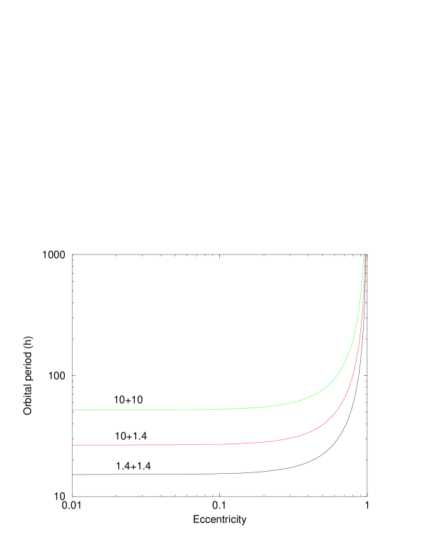
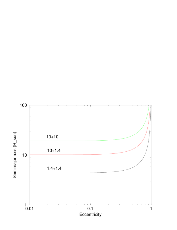
Figure 18: The maximal initial orbital period (in hours) of two point masses which will coalesce due to gravitational wave emission in a time interval shorter than $10^{10}$ years, as a function of the initial eccentricity $e_{0}$. The lines are calculated for 10M_⊙+10M_⊙ (BH+BH), 10M_⊙+1.4M_⊙ (BH+NS), and 1.4M_⊙+1.4M_⊙ (NS+NS).

Figure 19: The maximal initial semimajor axis (in R_⊙) of two point masses which will coalesce due to gravitational wave emission in a time interval shorter than $10^{10}$ years, as a function of the initial eccentricity $e_{0}$. The lines are calculated for 10M_⊙+10M_⊙ (BH+BH), 10M_⊙+1.4M_⊙ (BH+NS), and 1.4M_⊙+1.4M_⊙ (NS+NS).

A2 Mass transfer modes and mass loss in binary systems

The gravitational wave emission is the sole factor responsible for the change of orbital parameters of a pair of compact (degenerate) stars. However, at the early stages of binary evolution, it is the mass transfer between the components and the loss of matter and its orbital momentum that play dominant dynamical role. Strictly speaking, these processes should be treated hydrodynamically and they require complicated numerical calculations. However, binary evolution can also be described semi-qualitatively, using a simplified description in terms of point-like bodies. The change of their integrated physical quantities, such as masses, orbital angular momentum, etc. governs the evolution of the orbit. This description turns out to be successful in reproducing the results of more rigorous numerical calculations (see e.g. [40] for a review). In this approach, the key role is allocated to the total orbital angular momentum $J_{orb}$ of the binary.

Let star 2 lose matter at a rate $\dot{M}_{2}<0$ and let $\beta$ $(0\leq\beta\leq 1)$ be a fraction of the ejected matter which leaves the system (the rest falls on the first star), i.e. $\dot{M}_{1}=-(1-\beta)\dot{M}_{2}\geq 0$. Consider circular orbits with orbital angular momentum given by (A10). Differentiate both parts of Eq. (A10) by time $t$ and exclude $d\Omega/dt$ with the help of the third Kepler’s law (A3). This gives us the rate of change of the orbital separation:

$$\frac{\dot{a}}{a}=-2\left[1+(\beta-1)\frac{M_{2}}{M_{1}}-\frac{\beta}{2}\frac{M_{2}}{M}\right]\frac{\dot{M}_{2}}{M_{2}}+2\frac{\dot{J}_{orb}}{J_{orb}}$$ (A25)

One defines the mass transfer as conservative if both $\beta=0$ and $\dot{J}_{orb}=0$. The mass transfer is called non-conservative if at least one of these conditions is violated.

For massive binaries, which we are mostly interested in, it is important to distinguish some specific cases (modes) of mass transfer. They amount to: (1) conservative accretion mode, (2) non-conservative Jeans’s mode (or fast wind mode), (3) non-conservative isotropic re-emission, (4) sudden mass loss from one of the components during supernova explosion, and (5) common-envelope stage. Separately we consider orbit evolution due to (6) gravitational wave emission, which becomes the main factor for short-period compact binaries. For non-conservative modes, one can also introduce some subcases, such, for example, as a ring-like mode in which a circumbinary ring of expelled matter is being formed (e.g. [193]). Here, we will not go into the details of such subcases.

A2.1 Conservative accretion.

In the case of conservative accretion, matter from $M_{2}$ is fully deposited to $M_{1}$. The transfer process preserves the total mass $M=\hbox{\rm const}$ ($\beta=0$) and the orbital angular momentum $J_{orb}=\hbox{\rm const}$ of the system. It follows from Eq. (A25) that

$$M_{1}M_{2}\sqrt{a}=\hbox{\rm const}\,,$$

so that the initial and final binary separations are related as

$$\frac{a_{f}}{a_{i}}=\left(\frac{M_{1i}\,M_{2i}}{M_{1f}\,M_{2f}}\right)^{2}\,.$$ (A26)

The well-known “rule of thumb” for this case says that the orbit shrinks when the more massive component loses matter, and the orbit widens in the opposite situation. During such a mass exchange, the orbital separation passes through a minimum, if the masses become equal in course of the mass transfer.

A2.2 The Jeans (fast wind) mode.

In this mode the ejected matter completely escapes from the system, that is, $\beta=1$. The escape of matter can take place either in a spherically symmetric way or in the form of bipolar jets moving from the system at high velocity. In both cases, matter carries away some amount of the total orbital momentum proportional to the orbital angular momentum $J_{2}=(M_{1}/M)J_{orb}$ of the mass loosing star (we neglect a possible proper rotation of the star, see [194]). For the loss of orbital momentum $\dot{J}_{orb}$ it is reasonable to take

$$\dot{J}_{orb}=\frac{\dot{M}_{2}}{M_{2}}J_{2}\,.$$ (A27)

In the case $\beta=1$, Eq. (A25) can be written as

$$\frac{(\Omega a^{2})\,\dot{}}{\Omega a^{2}}=\frac{\dot{J}_{orb}}{J_{orb}}-\frac{M_{1}\dot{M}_{2}}{MM_{2}}\,.$$ (A28)

Then Eq. (A28) in conjunction with Eq. (A27) give $\Omega a^{2}=\hbox{\rm const}$, that is, $\sqrt{GaM}=\hbox{\rm const}$. Thus, as a result of such a mass loss, the change in orbital separation is

$$\frac{a_{f}}{a_{i}}=\frac{M_{i}}{M_{f}}\,.$$ (A29)

Since the total mass decreases, the orbit always widens.

A2.3 Isotropic re-emission.

The matter lost by star 2 can first accrete to star 1, and then, a fraction $\beta$ of the accreted matter, can be expelled from the system. This happens when a massive star transfers matter to a compact star on the thermal timescale ($<10^{6}$ years). The accretion luminosity may exceed the Eddington luminosity limit, and the radiation pressure pushes the infalling matter away from the system, in a manner similar to the spectacular example of the SS 433 binary system. In this mode of the mass transfer, the binary orbital momentum carried away by the expelled matter is determined by the orbital momentum of the accreting star $M_{1}$, rather than by the orbital momentum of the mass-loosing star $M_{2}$. The orbital momentum loss can be written as

$$\dot{J}_{orb}=\beta\frac{\dot{M}_{2}}{M_{1}}J_{1}\,,$$ (A30)

where $J_{1}=(M_{2}/M)J_{orb}$ is the orbital momentum of the star $M_{1}$. In the limiting case when all the mass attracted by $M_{1}$ is fully pushed away, $\beta=1$, Eq. (A30) simplifies to

$$\frac{\dot{J}_{orb}}{J_{orb}}=\frac{\dot{M_{2}}M_{2}}{M_{1}M}\,.$$ (A31)

After substitution of this formula into Eq. (A25) and integration over time, one arrives at

$$\frac{a_{f}}{a_{i}}=\frac{M_{i}}{M_{f}}\left(\frac{M_{2i}}{M_{2f}}\right)^{2}\exp{\left(-2\,\frac{M_{2i}-M_{2f}}{M_{1}}\right)}\,.$$ (A32)

The exponential term makes this mode of the mass transfer very sensitive to the components mass ratio. If $M_{1}/M_{2}\ll 1$, the separation $a$ between the stars may decrease so greatly that the approximation of point masses becomes invalid. The tidal orbital instability (Darwin instability) may set in, and the compact star may start spiraling toward the companion star center (the common envelope stage; see section A2.5 below).

A2.4 Supernova explosion.

Supernova explosion in a binary system occurs on a timescale much shorter than the orbital period, so the loss of mass is practically instantaneous. This case can be treated analytically (e.g. [195, 196, 79]). In general, the loss of matter and radiation is aspherical, so that the remnant of the supernova explosion (neutron star or black hole) acquires some recoil velocity called kick velocity ${\mathbf{w}}$. In a binary, kick velocity should be added to the orbital velocity of the pre-supernova star.

The usual treatment proceeds as follows. Let us consider a pre–SN binary with initial masses $M_{1}$ and $M_{2}$. The stars move in a circular orbit with orbital separation $a_{i}$ and relative velocity ${\mathbf{V}}_{i}$. The star $M_{1}$ explodes leaving a compact remnant of mass $M_{c}$. The total mass of the binary decreases by the amount $\Delta M=M_{1}-M_{c}$. The compact star acquires some kick velocity ${\mathbf{w}}$. Unless the binary is disrupted, it will end up in a new orbit with eccentricity $e$, major semiaxis $a_{f}$, and the angle $\theta$ between the orbital planes before and after the explosion. In general, the new barycenter will also receive some velocity, but we neglect this motion. The goal is to evaluate the parameters $a_{f}$, $e$, and $\theta$.

It is convenient to work in an instantaneous reference frame centered on $M_{2}$ right at the time of explosion. The x–axis is the line from $M_{2}$ to $M_{1}$, the y–axis points in the direction of ${\mathbf{V}}_{i}$, and the z–axis is perpendicular to the orbital plane. In this frame, the pre–SN relative velocity is ${\mathbf{V}}_{i}=(0,V_{i},0)$, where $V_{i}=\sqrt{G(M_{1}+M_{2})/a_{i}}$ (Eq. (A9). The initial total orbital momentum is ${\mathbf{J}}_{i}=\mu_{i}a_{i}(0,0,-V_{i})$. The explosion is considered to be instantaneous. Right after the explosion, the position vector of the exploded star $M_{1}$ has not changed: ${\mathbf{r}}=(a_{i},0,0)$. However, other quantities has changed: ${\mathbf{V}}_{f}=(w_{x},V_{i}+w_{y},w_{z})$ and ${\mathbf{J}}_{f}=\mu_{f}a_{i}(0,w_{z},-(V_{i}+w_{y}))$, where ${\mathbf{w}}=(w_{x},w_{y},w_{z})$ is the kick velocity and $\mu_{f}=M_{c}M_{2}/(M_{c}+M_{2})$ is the reduced mass of the system after explosion. The parameters $a_{f}$ and $e$ are being found from equating the total energy and the absolute value of orbital momentum at the initial circular orbit to their expressions at the resulting elliptical orbit (see Eqs. (A6), (A10), and (A8)):

$$\mu_{f}\frac{V_{f}^{2}}{2}-\frac{GM_{c}M_{2}}{a_{i}}=-\frac{GM_{c}M_{2}}{2a_{f}},$$ (A33)

$$\mu_{f}a_{i}\sqrt{w_{z}^{2}+(V_{i}+w_{y})^{2}}=\mu_{f}\sqrt{G(M_{c}+M_{2})a_{f}(1-e^{2})}.$$ (A34)

For the resulting $a_{f}$ and $e$ one finds

$$\frac{a_{f}}{a_{i}}=\left(2-\chi\left[\frac{w_{x}^{2}+w_{z}^{2}+(V_{i}+w_{y})^{2}}{V_{i}^{2}}\right]\right)^{-1}$$ (A35)

and

$$1-e^{2}=\chi\frac{a_{i}}{a_{f}}\left[\frac{w_{z}^{2}+(V_{i}+w_{y})^{2}}{V_{i}^{2}}\right]$$ (A36)

where $\chi\equiv(M_{1}+M_{2})/(M_{c}+M_{2})\geq 1$. The angle $\theta$ is defined by

$$\cos\theta=\frac{{\mathbf{J}}_{f}\cdot{\mathbf{J}}_{i}}{|{\mathbf{J}}_{f}|~{}|{\mathbf{J}}_{i}|},$$

which results in

$$\cos\theta=\frac{V_{i}+w_{y}}{\sqrt{w_{z}^{2}+(V_{i}+w_{y})^{2}}}.$$ (A37)

The condition of disruption of the binary system depends on the absolute value $V_{f}$ of the final velocity, and on the parameter $\chi$. The binary disrupts if its total energy defined by the left-hand-side of Eq. (A33) becomes non-negative or, equivalently, if its eccentricity defined by Eq. (A36) becomes $e\geq 1$. From either of these requirements one derives the condition of disruption:

$$\frac{V_{f}}{V_{i}}\geq\sqrt{\frac{2}{\chi}}.$$ (A38)

The system remains bound if the opposite inequality is satisfied. Eq. (A38) can also be written in terms of the escape (parabolic) velocity $V_{e}$ defined by the requirement

$$\mu_{f}\frac{V_{e}^{2}}{2}-\frac{GM_{c}M_{2}}{a_{i}}=0.$$

Since $\chi=M/(M-\Delta M)$ and $V_{e}^{2}=2G(M-\Delta M)/a_{i}=2V_{i}^{2}/\chi$, one can write Eq. (A38) in the form

$$V_{f}\geq V_{e}.$$ (A39)

The condition of disruption simplifies in the case of a spherically symmetric SN explosion, that is, when there is no kick velocity, ${\mathbf{w}}=0$, and, therefore, $V_{f}=V_{i}$. In this case, Eq. (A38) reads $\chi\geq 2$, which is equivalent to $\Delta M\geq M/2$. Thus, the system unbinds if more than a half of mass of the binary is lost. In other words, the resulting eccentricity

$$e=\frac{M_{1}-M_{c}}{M_{c}+M_{2}}\,$$ (A40)

following from (A35), (A36), and ${\mathbf{w}}=0$ becomes larger than 1, if $\Delta M>M/2$. So far, we have considered an originally circular orbit. If the pre–SN star moves in an originally eccentric orbit, the condition of disruption of the system under symmetric explosion reads

$$\Delta M=M_{1}-M_{c}>\frac{1}{2}\frac{r}{a_{i}}\,,$$

where $r$ is the distance between the components at the moment of explosion.

A2.5 Common envelope stage.

This is a very important stage in binary evolution. A possibility of this stage was first suggested in [197]. Generally, it occurs in binary systems where the mass transfer from the mass-losing star is high, and the companion cannot accrete all the matter. The common envelope stage appears unavoidable on the observational grounds. The evidence for a dramatic orbital angular momentum decrease at some preceding evolutionary stage follows from observations of certain types of close binary stars. They include cataclysmic variables, in which a white dwarf accretes matter from a small red dwarf main-sequence companion, planetary nebulae with double cores, low-mass X-ray binaries and X-ray transients (neutron stars and black holes accreting matter from low-mass main-sequence dwarfs). The radii of progenitors of compact stars in these binaries typically should have been 100–1000 solar radii, that is, much larger than the observed binary separations. This testifies to some dramatic reduction of the orbital momentum at earlier stages of evolution and eventual removal of the common envelope.

There is no exact criterion for the formation of a common envelope. However, a high mass overflow onto a compact star from a normal star is always expected when the normal star leaves the main-sequence and develops a convective envelope. The critical mass ratio for the unstable Roche lobe overflow depends on specifics of the stars, but is close to 1. Another way for the formation of a common envelope is direct penetration of a compact star into the dense outer layers of the companion. This can happen as a result of the Darwin tidal orbital instability in binaries [198, 199], or when a compact remnant of supernova explosion with appropriately directed kick velocity finds itself in an elliptic orbit whose minimum periastron distance $a_{f}(1-e)$ is smaller than the stellar radius of the companion.

A simplified treatment of the common envelope stage is usually done as follows [200]. The orbital evolution of the compact star $M_{c}$ inside the envelope of the normal star $M_{1}$ is driven by the dynamical friction drag. This leads to a gradual spiral-in process of the compact star. The released orbital energy $\Delta E_{orb}$, or a fraction of it, can become numerically equal to the binding energy $E_{bind}$ of the envelope with the rest of the binary system. It is usually assumed that this equality provides a condition for expulsion of the common envelope. What remains of the normal star $M_{1}$ is its stellar core $M_{sc}$. The final orbital parameters are being derived from the condition $E_{bind}=\alpha_{CE}\Delta E_{orb}$, where $\alpha_{CE}$ is the efficiency parameters less or equal to one. This condition reads

$$\frac{GM_{1}(M_{1}-M_{sc})}{\lambda R_{L}}=\alpha_{CE}\left(\frac{GM_{c}M_{sc}}{2a_{f}}-\frac{GM_{1}M_{c}}{2a_{i}}\right),$$ (A41)

where $a_{i}$ and $a_{f}$ are the initial and the final orbital separations, $\lambda$ is a numerical coefficient of order 1. $R_{L}$ is the Roche lobe radius of the normal star approximated by [201]

$$\frac{R_{L}}{a_{i}}=\frac{0.49}{0.6+q^{2/3}\ln(1+q^{-1/3})}$$ (A42)

and $q\equiv M_{1}/M_{2}$. From Eq. (A41) one derives

$$\frac{a_{f}}{a_{i}}=\frac{M_{sc}}{M_{1}}\left(1+\frac{2a_{i}}{\lambda\alpha_{CE}R_{L}}\frac{M_{1}-M_{sc}}{M_{c}}\right)^{-1}\mathrel{\mathchoice{\vbox{\offinterlineskip\halign{\hfil$\displaystyle#$\hfil\cr<\cr\vskip 1.5pt\cr\sim\cr}}}{\vbox{\offinterlineskip\halign{\hfil$\textstyle#$\hfil\cr<\cr\vskip 1.0pt\cr\sim\cr}}}{\vbox{\offinterlineskip\halign{\hfil$\scriptstyle#$\hfil\cr<\cr\vskip 0.5pt\cr\sim\cr}}}{\vbox{\offinterlineskip\halign{\hfil$\scriptscriptstyle#$\hfil\cr<\cr\vskip 0.5pt\cr\sim\cr}}}}\frac{M_{sc}}{M_{1}}\frac{M_{c}}{\Delta M}\,,$$ (A43)

where $\Delta M=M_{1}-M_{sc}$. Recent studies (e.g. [202, 68]) show that $\alpha_{CE}\lambda$ falls within the range from 0.5 to 2. The mass $M_{sc}$ of a helium core of a massive star is (see [203])

$$M_{\rm He}\approx 0.073(M_{1}/M_{\odot})^{1.42},$$ (A44)

so the orbital separation during the common envelope stage may decrease as much as by factor 30–60.

A3 Post-Newtonian expansions of GW flux and energy

The gravitational wave flux escaping a system of two compact stars in quasi-circular orbit when their orbital frequency is $f_{\rm orb}$ (the dominant GW frequency being $f=2f_{\rm orb}$), is given by [204, 205, 206, 207]

$${\cal F}(v) = \frac{32\eta^{2}v^{10}}{5}\Biggl{[}1-\left(\frac{1247}{336}+\frac{35\eta}{12}\right)v^{2}+4\pi v^{3}$$ (A45)

$$- \left(\frac{44711}{9072}+\frac{9271\eta}{504}+\frac{65\eta^{2}}{18}\right)v^{4}-\left(\frac{8191}{672}+\frac{535\eta}{24}\right)\pi v^{5}\Biggr{]}$$

where $v=(\pi Mf)^{1/3}$ is the relative velocity of the two stars and $\eta=M_{1}M_{2}/M^{2}$ is the symmetric mass ratio. The $\eta$-parameter takes a maximum values of 1/4 when the two masses are equal. It characterises the extent to which two-body effects in the system are important. The relativistic energy $E(v)$ of the system is given by

$$E(v)=-\frac{\eta v^{2}}{2}\left[1-\left(\frac{9+\eta}{12}\right)v^{2}-\left(\frac{81-57\eta+\eta^{2}}{24}\right)v^{4}\right].$$ (A46)

Solving the differential equations in Eq. (127) for time and phase in terms of $v$ gives the following equations:

$$t(v) = -\frac{5M}{256\eta v^{8}}\Biggl{[}1+\left(\frac{743}{252}+\frac{11\eta}{3}\right)v^{2}-\frac{32\pi}{5}v^{3}$$ (A47)

$$+ \left(\frac{3058673}{508032}+\frac{5429\eta}{504}+\frac{617\eta^{2}}{72}\right)v^{4}-\left(\frac{7729}{252}+\eta\right)\pi v^{5}\Biggr{]},$$

$$\phi(v) = -\frac{1}{16\eta v^{5}}\Biggl{[}1+\left(\frac{3715}{1008}+\frac{55\eta}{12}\right)v^{2}-10\pi v^{3}+\left(\frac{15293365}{1016064}+\frac{27145\eta}{1008}+\frac{3085\eta^{2}}{144}\right)v^{4}$$ (A48)

$$+ \left(\frac{38645}{672}+\frac{15\eta}{8}\right)\pi\ln\left(\frac{v}{v_{\rm lso}}\right)v^{5}\Biggr{]}.$$

One can invert the first of the equations above to express $v$ in terms of a post-Newtonian expansion in $t$ and then use the resulting expression in the second equation to arrive at an explicit phasing formula. Introducing a new time parameter $\theta$ defined by $\theta=[\eta(t_{\rm lso}-t)/(5M)]^{-1/8},$ where $t_{\rm lso}$ is a reference time taken to be the time at which the GW frequency is equal to twice the orbital frequency at the last stable circular orbit, we find

$$\phi(\theta) = -\frac{2}{\eta\theta^{5}}\Biggl{[}1+\left(\frac{3715}{8064}+\frac{55\eta}{96}\right)\theta^{2}-\frac{3\pi}{4}\theta^{3}+\left(\frac{9275495}{14450688}+\frac{284875\eta}{258048}+\frac{1855\eta^{2}}{2048}\right)\theta^{4}$$ (A49)

$$+ \left(\frac{38645}{21504}+\frac{15\eta}{256}\right)\pi\ln\left(\frac{\theta}{\theta_{\rm lso}}\right)\theta^{5}\Biggr{]}.$$

References

- 1. Weber J General Relativity and Gravitational Waves (New York: Interscience, 1961)
- 2. Landau L D, Lifshitz E M The classical theory of fields (Oxford, England: Pergamon Press, 1975)
- 3. Misner C W, Thorne K S, Wheeler J A Gravitation (San Francisco: W. H. Freeman and Company, 1973)
- 4. Thorne K S in Three Hundred Years of Gravitation (Ed. S W Hawking, W Israel) (Cambridge: Cambridge University Press, 1987) p. 330
- 5. Thorne K S in Particle and Nuclear Astrophysics and Cosmology in the Next Millenium (Ed. E W Kolb, R D Peccei) (Singapore: World Scientific Publ., 1995) p. 160
- 6. Schutz B F Class. Quant. Gravity 16 A131 (1999)
- 7. Braginsky V B, Rudenko V N Usp. Fiz. Nauk 100 395 (1970)
- 8. Grishchuk L P Usp. Fiz. Nauk 121 629 (1977) [Sov. Phys. Usp. 20 319 (1977)]
- 9. Grishchuk L P Usp. Fiz. Nauk 156 297 (1988) [Sov. Phys. Usp. 31 940 (1988)]
- 10. Will C M Usp. Fiz. Nauk 164 765 (1994) [Phys. Usp. 37 697 (1994)]
- 11. King A R in Relativistic Gravitation and Gravitational Radiation (Cambridge: Cambridge University Press, 1997) p. 105
- 12. Taylor J Rev. Mod. Phys. 66 711 (1994)
- 13. Danzmann K et al. in First Edoardo Amaldi Conference on Gravitational Wave Experiments (Ed. E Coccia, G Pizzella, F Ronga) (Singapore: World Scientific, 1995) p. 100
- 14. Bradaschia C et al. Nucl. Instr. Meth. A 289 518 (1990)
- 15. Abramovici A et al. Science 256 325 (1992)
- 16. Bender P et al. LISA: Pre–Phase A Report, Second Edition, Garching, Germany, 1998
- 17. LIGO II Conceptual Project Book, 1999, LIGO-M990288-00-M
- 18. Taylor J H, Manchester R N, Lyne A G Astrophys. J. Suppl. 88 529 (1993)
- 19. D’Amico N et al. Preprint astro–ph/9911482 (1999)
- 20. Camilo F et al. in ASP Conf. Ser. 202: IAU Colloq. 177: Pulsar Astronomy — 2000 and Beyond (San Francisco: Astronomical Society of the Pacific, 2000) p. 3
- 21. Cherepashchuk A M Usp. Fiz. Nauk 166 809 (1996) [Phys. Usp. 39 759 (1996)]
- 22. Thorsett S E, Chakrabarty D Astrophys. J. 512 288 (1999)
- 23. Nice D J, Sayer R W, Taylor J H Astrophys. J. Lett. 466 L87 (1996)
- 24. Phinney E S Astrophys. J. Lett. 380 L17 (1991)
- 25. Narayan R, Piran T, Shemi A Astrophys. J. Lett. 379 L17 (1991)
- 26. Curran S J, Lorimer D R Montly Not. RAS 276 347 (1995)
- 27. van den Heuvel E P J, Lorimer D R Montly Not. RAS 283 L37 (1996)
- 28. Bailes M in IAU Symp. 165: Compact Star in Binaries (Ed. J A van Paradijs, E P J van den Heuvel, E Kuulkers) (Dordrecht: Kluwer, 1996) p. 213
- 29. Arzoumanian Z, Cordes J M, Wasserman I Astrophys. J. 520 696 (1999)
- 30. Stairs I H et al. Astrophys. J. 505 352 (1998)
- 31. Kalogera V, Lorimer D R Astrophys. J. 530 890 (2000)
- 32. Clark J P A, van den Heuvel E P J, Sutantyo W Astron. Astrophys. 72 120 (1979)
- 33. Lipunov V M, Postnov K A, Prokhorov M E Astron. Astrophys. 176 L1 (1987)
- 34. Hils D, Bender P L, Webbink R F Astrophys. J. 360 75 (1990)
- 35. Tutukov A V, Yungelson L R Astron. Zhurn. 70 812 (1993) [Astron. Rep. 37 411 (1993)]
- 36. Lipunov V M et al. Astron. Astrophys. 298 677 (1995)
- 37. Portegies Zwart S F, Spreeuw H N Astron. Astrophys. 312 670 (1996)
- 38. Lipunov V M, Postnov K A, Prokhorov M E Astrophys. Scape Phys. Rev. 9 1 (1996)
- 39. Portegies Zwart S F, Yungelson L R Astron. Astrophys. 332 173 (1998)
- 40. van den Heuvel E P J in Interacting Binaries (Ed. H Nussbaumer, A Orr) (Berlin: Springer, 1994) p. 263
- 41. Abt H A Ann. Rev. Astron. Astrophys. 21 343 (1983)
- 42. Salpeter E E Astrophys. J. 121 161 (1955)
- 43. Popova E I, Tutukov A V, Yungelson L R Astrophys. Space Sci. 88 55 (1982)
- 44. Trimble V Nature 303 137 (1983)
- 45. Lipunov V M, Postnov K A, Prokhorov M E Astron. Astrophys. 310 489 (1996)
- 46. Kaspi V M et al. Nature 381 584 (1996)
- 47. Prokhorov M E, Postnov K A Pis’ma Astron. Zhurn. 23 503 (1997) [Astron. Lett. 23 439 (1997)]
- 48. Karastergiou A, Kramer M, Wex N, von Hoensbroech A in ASP Conf. Ser. 202: IAU Colloq. 177: Pulsar Astronomy — 2000 and Beyond (San Francisco: Astronomical Society of the Pacific, 2000) p. 125
- 49. Karastergiou A, Kramer M, Wex N, von Hoensbroech A Preprint astro–ph/0002099 (2000)
- 50. Iben J, Tutukov A V Astrophys. J. 456 738 (1996)
- 51. Portegies Zwart S F, van den Heuvel E P J New Astron. 4 355 (1999)
- 52. van den Heuvel E P J, van Paradijs J Astrophys. J. 483 399 (1997)
- 53. Tauris T M, van den Heuvel E P J in ASP Conf. Ser. 202: IAU Colloq. 177: Pulsar Astronomy — 2000 and Beyond (San Francisco: Astronomical Society of the Pacific, 2000) p. 595
- 54. Tauris A, van den Heuvel E P J Preprint astro–ph/0001015 (2000)
- 55. Lai D Preprint astro–ph/9912522 (1999)
- 56. Dorofeev O F, Rodionov V N, Ternov I M Pis’ma Astron. Zhurn. 11 302 (1985) [Sov. Astron. Lett. 11 123 (1985)]
- 57. Bisnovatyi–Kogan G S Astron. Astroph. Trans. 3 287 (1993)
- 58. Lyne A G, Lorimer D R Nature 369 127 (1994)
- 59. Blaauw A, Ramachandran R J. Astron. Astrophys. 19 19 (1998)
- 60. Frail D A, Goss W M, Whiteoak J B Z Astrophys. J. 437 781 (1994)
- 61. Lorimer D R 1997, private communication
- 62. Hansen B M S, Phinney E S Montly Not. RAS 291 569 (1997)
- 63. Lipunov V M, Postnov K A, Prokhorov M E Montly Not. RAS 288 245 (1997)
- 64. Belczynski K, Bulik T Astron. Astrophys. 346 91 (1999)
- 65. Bagot P Astron. Astrophys. 322 533 (1997)
- 66. Wettig T, Brown G E New Astron. 1 17 (1996)
- 67. Terman J L, Taam R E, Savage C O Montly Not. RAS 281 552 (1996)
- 68. Rasio F A, Livio M Astrophys. J. 471 366 (1996)
- 69. van den Heuvel E P J, Habets G M H J Nature 309 598 (1984)
- 70. Woosley S E, Langer N, Weaver T A Astrophys. J. 448 315 (1995)
- 71. Portegies Zwart S F, Verbunt F, Ergma E Astron. Astrophys. 321 207 (1997)
- 72. Timmes F X, Woosley S E, Weaver T A Astrophys. J. 457 834 (1996)
- 73. Bethe H A, Brown G E Astrophys. J. 517 318 (1999)
- 74. Fryer C L Astrophys. J. 522 413 (1999)
- 75. Fryer C L, Kalogera V Preprint astro–ph/9911312 (1999)
- 76. Nelemans G, Tauris T M, van den Heuvel E P J Astron. Astrophys. 352 L87 (1999)
- 77. Kuranov A G, Postnov K A, Prokhorov M E 2000, submitted to Astron. Rep.
- 78. Schaller G, Schaerer D, Meynet G, Maeder A Astron. Astrophys. Suppl. 96 269 (1992)
- 79. Yamaoka H, Shigeyama T, Nomoto K Astron. Astrophys. 267 433 (1993)
- 80. Brandt N, Podsiadlowski P Montly Not. RAS 274 461 (1995)
- 81. Lipunov V M, Postnov K A, Prokhorov M E Pis’ma Astron. Zhurn. 23 563 (1997) [Astron. Lett. 23 492 (1997)]
- 82. Tutukov A V, Yungelson L R Montly Not. RAS 260 675 (1993)
- 83. Fukugita M, Hogan C J, Peebles P J E Astrophys. J. 503 518 (1998)
- 84. Edmunds M G in ASP Conf. Ser.:The Low Surface Brightness Universe Vol. 170 (San Francisco: Astronomical Society of the Pacific, 1999) p. 383
- 85. Olive K A Nucl. Phys. B Proc. Suppl. 80 79 (2000)
- 86. Lipunov V M et al. Astrophys. J. 454 593 (1995)
- 87. Vanbeveren D et al. New Astron. 3 443 (1998)
- 88. Flanagan É É, Hughes S A Phys. Rev. D 57 4535 (1998)
- 89. Postnov K A, Prokhorov M E Preprint astro-ph/9903193 (1999)
- 90. Kalogera V Preprint astro–ph/9911417 (1999)
- 91. Müller E Class. Quant. Gravity 14 1455 (1997)
- 92. Palomba C Preprint astro-ph/0003321 (2000)
- 93. Burrows A, Hayes J C Amer. Astr. Soc. Meeting 187 1704 (1995)
- 94. Nazin S N, Postnov K A Astron. Astrophys. 317 L79 (1997)
- 95. Braginskii V B, Grishchuk L P Zh. Eksp. Teor. Fiz. 89 744 (1985)
- 96. Braginskii V B, Thorne K S Nature 327 123 (1987)
- 97. Bonnell I A, Pringle J E Montly Not. RAS 273 L12 (1995)
- 98. Schutz B F Preprint gr–qc/9802020 (1998)
- 99. Burrows A, Hayes J Phys. Rev. Lett. 76 352 (1996)
- 100. Müller E, Janka H T Astron. Astrophys. 317 140 (1997)
- 101. Buonanno A, Damour T Preprint gr-qc/0001013 (2000)
- 102. Alcock C et al. Astrophys. J. 486 697 (1997)
- 103. Nakamura T, Sasaki M, Tanaka T, Thorne K S Astrophys. J. Lett. 487 L139 (1997)
- 104. Echeverria F Phys. Rev. D 40 3194 (1989)
- 105. Chandrasekhar S Phys. Rev. Lett. 24 611 (1970)
- 106. Friedman J L, Schutz B F Astrophys. J. 222 281 (1978)
- 107. Andersson N Astrophys. J. 502 708 (1998)
- 108. Andersson N, Kokkotas K, Schutz B F Astrophys. J. 510 846 (1999)
- 109. Owen B J et al. Phys. Rev. D 58 14834 (1998)
- 110. Bildsten L Astrophys. J. Lett. 501 89 (1998)
- 111. Kulkarni S R et al. in X–ray Binaries and Recycled Pulsars Vol. 377 (Ed. E P J van den Heuvel, S A Rappaport) (Dordrecht, The Netherlands: Kluwer Academic Publisher, 1992) p. 99
- 112. Caron B et al. Nucl. Phys. B Proc. Suppl. 54 167 (1997)
- 113. Giampieri G, Polnarev A G Montly Not. RAS 291 149 (1997)
- 114. Lipunov V M, Postnov K A Astron. Zhurn. 64 438 (1987) [Sov. Astron. 31 228 (1987)]
- 115. Schneider R, Ferrari V, Mattarese S, Portegies Zwart S Preprint astro–ph/0002055 (2000)
- 116. Marsh T R, Dhillon V S, Duck S R Montly Not. RAS 275 828 (1995)
- 117. Iben J, Tutukov A V Astrophys. J. Suppl. 54 335 (1984)
- 118. Branch D et al. Publ. Astron. Soc. Pacif. 107 1019 (1995)
- 119. Tammann G A, Loeffler W, Schroeder A Astrophys. J. Suppl. 92 487 (1994)
- 120. van den Bergh S, McClure R D Astrophys. J. 425 205 (1994)
- 121. Postnov K A, Prokhorov M E Astrophys. J. 494 674 (1998)
- 122. Kosenko D I, Postnov K A Astron. Astrophys. 336 786 (1998)
- 123. Kosenko D I, Postnov K A Astron. Astrophys. 355 1209 (2000)
- 124. Grishchuk L P Zh. Eksp. Teor. Fiz. 67 825 (1974) [Sov. Phys. JETP 40 409 (1975)]
- 125. Grishchuk L P Ann. NY Acad. Sci. 302 439 (1977)
- 126. Knight P L in Quantum Fluctuations (Ed. S Reynaud, E Giacobino, J Zinn–Justin) (Amsterdam: Elsevier Science, 1997) p. 5
- 127. Grishchuk L P, Sidorov Y V Class. Quant. Gravity 6 L161 (1989)
- 128. Grishchuk L P, Sidorov Y V Phys. Rev. D 42 3413 (1990)
- 129. Grishchuk L P in Workshop on Squeezed States and Uncertainty Relations (New York: NASA Conf. Publ. No. 3135, 1992) p. 329
- 130. Grishchuk L P in Quantum Fluctuations (Ed. S Reynaud, E Giacobino, J Zinn–Justin) (Amsterdam: Elsevier Science, 1997) p. 541
- 131. Schleich W, Wheeler J A Opt. Soc. Amer. J. B 4 1715 (1987)
- 132. Schleich W, Horowicz R J, Varro S Phys. Rev. A 40 7405 (1989)
- 133. Zeldovich Y B, Novikov I D Relativistic Astrophysics. Volume 2 — The Structure and Evolution of the Universe. (Chicago: University of Chicago Press, 1983)
- 134. Giovannini M Phys. Rev. D 58 14630 (1998)
- 135. Grishchuk L P Preprint gr–qc/9810055 (1998)
- 136. Veneziano G Phys. Lett. B 256 287 (1991)
- 137. Gasperini M, Veneziano G Astropart. Phys. 1 317 (1993)
- 138. Gasperini M, Giovannini M Phys. Rev. D 47 1519 (1993)
- 139. Creighton T Preprint gr–qc/9907045 (1999)
- 140. Smoot G F et al. Astrophys. J. Lett. 396 L1 (1992)
- 141. Bennett C L et al. Astrophys. J. Lett. 464 L1 (1996)
- 142. Melchiorri A, Sazhin M V, Shulga V V, Vittorio N Astrophys. J. 518 562 (1999)
- 143. Grishchuk L P Phys. Rev. D 50 7154 (1994)
- 144. Grishchuk L P in Current Topics in Astrofundamental Physics: Primordial Cosmology (Ed. N Sanchez, A Zichichi) (Dordrecht: Kluwer Academic Publishers, 1998) p. 539
- 145. Grishchuk L P Preprint gr–qc/9801011 (1998)
- 146. Grishchuk L P Class. Quant. Gravity 14 1445 (1997)
- 147. Tegmark M, Zaldarriaga M Preprint astro-ph/0002091 (2000)
- 148. Kolb E W, Turner M S The Early Universe (Reading, Massachusetts: Addison-Wesley, 1990)
- 149. Martin J, Schwarz D J Preprint astro–ph/9911225 (1999)
- 150. Hawking S W, Hertog T, Reall H S Phys. Rev. D 62 9ed (2000)
- 151. Hough J et al. GEO600 Proposal, 1994
- 152. Larson S L, Hiscock W A, Hellings R W Phys. Rev. D 62 231 (2000)
- 153. Gravitational Wave Experiments (Ed. E Coccia, G Pizzella, F Ronga) (Singapore: World Scientific, 1995)
- 154. Gravitational Waves: Sources and Detection (Ed. I Giufolini, F Fidecaro) (Singapore: World Scientific, 1997)
- 155. AIP Conference Proceedings: Laser Interferometer Space Antenna Vol. 456 (Ed. W M Folkner) (Melvill, NY: AIP, 1998)
- 156. Grishchuk L P Sov. Phys. JETP Lett. 23 293 (1976)
- 157. Michelson P F Montly Not. RAS 227 933 (1987)
- 158. Christensen N Phys. Rev. D 46 5250 (1992)
- 159. Flanagan É É Phys. Rev. D 48 2389 (1993)
- 160. Allen B in Relativistic Gravitation and Gravitational Radiation (Ed. J A Marck, J P Lasota) (Cambridge: Cambridge University Press, 1997) p. 373
- 161. Allen B, Flanagan É É, Papa M A Phys. Rev. D 61 024024 (2000)
- 162. Tsubono K in First Edoardo Amaldi Conference on Gravitational Wave Experiments (Singapore: World Scientific, 1995) p. 112
- 163. Lück H et al. Class. Quant. Gravity 14 1471 (1997)
- 164. Caron B et al. Class. Quant. Gravity 14 1461 (1997)
- 165. Meers B, MacDonald N Phys. Rev. A 40 3754 (1989)
- 166. Dhurandhar S V, Tinto M Montly Not. RAS 234 663 (1988)
- 167. Helstrom C W Statistical Theory of Signal Detection (London: Pergamon Press, 1968)
- 168. Schutz B F in The Detection of Gravitational Waves (Ed. D G Blair) (Cambridge, England: Cambridge University Press, 1991) p. 406
- 169. Cutler C et al. Phys. Rev. D 70 2984 (1993)
- 170. Damour T, Iyer B R, Sathyaprakash B S Phys. Rev. D 57 885 (1998)
- 171. Damour T, Iyer B R, Sathyaprakash B S, in preparation
-
172.
Allen B et al. GRASP software package,
( http://www.lsc-group.phys.uwm.edu/~ballen/grasp-distribution/ ) - 173. Poisson E Phys. Rev. D 52 5719 (1995)
- 174. Damour T, Iyer B R, Sathyaprakash B S, submitted to Phys. Rev. D
- 175. Sathyaprakash B S, Dhurandhar S V Phys. Rev. D 44 3819 (1991)
- 176. Schutz B F Nature 323 310 (1986)
- 177. Blanchet L, Sathyaprakash B S Class. Quant. Gravity 11 2807 (1994)
- 178. Blanchet L, Sathyaprakash B S Phys. Rev. D 74 1067 (1995)
- 179. Owen B J Phys. Rev. D 53 6749 (1996)
- 180. Balasubramanian R, Sathyaprakash B S, Dhurandhar S V Phys. Rev. D 53 3033 (1996)
- 181. Owen B J, Sathyaprakash B S Phys. Rev. D 60 022002 (1999)
- 182. Brady P R, Creighton T, Cutler C, Schutz B F Phys. Rev. D 57 2101 (1998)
- 183. Brady P R, Creighton T, private communication
- 184. Schutz B F, Papa M A Preprint gr–qc/9905018 (1999)
- 185. Nicholson D, Vecchio A Phys. Rev. D 57 4588 (1998)
- 186. Balasubramanian R, Sathyaprakash B S, Dhurandhar S V Phys. Rev. D 54 1860 (1996)
- 187. Cutler C, Flanagan É É Phys. Rev. D 49 2658 (1994)
- 188. Poisson E, Will C M Phys. Rev. D 52 848 (1995)
- 189. Sathyaprakash B S in Relativistic Gravitation and Gravitational Radiation (Cambridge: Cambridge University Press, 1997) p. 361
- 190. Landau L D, Lifshitz E M Mechanics (Oxford, England: Pergamon Press, 1969)
- 191. Babak S V, Grishchuk L P Phys. Rev. D 61 024038 (1999)
- 192. Peters P C Phys. Rev. B 136 1224 (1964)
- 193. Soberman G E, Phinney E S, van den Heuvel E P J Astron. Astrophys. 327 620 (1997)
- 194. van den Heuvel E P J in Formation and Evolution of X-ray Binaries (Cambridge: Cambridge University Press, 1983) p. 303
- 195. Blaauw A Bull. Astron. Inst. Netherland 15 265 (1961)
- 196. Flannery B P, van den Heuvel E P J Astron. Astrophys. 39 61 (1975)
- 197. Paczynski B IAU Symp. 73 75 (1976)
- 198. Counselman C C Astrophys. J. 180 307 (1973)
- 199. Bagot P Astron. Astrophys. 314 576 (1996)
- 200. Webbink R F Astrophys. J. 277 355 (1984)
- 201. Eggleton P P Astrophys. J. 268 368 (1983)
- 202. van den Heuvel E P J Astron. Astrophys. 291 L39 (1994)
- 203. Iben J, Tutukov A V Astrophys. J. Suppl. 58 661 (1985)
- 204. Blanchet L et al. Phys. Rev. D 74 3515 (1995)
- 205. Blanchet L, Damour T, Iyer B R Phys. Rev. D 51 5360 (1995)
- 206. Will C M, Wiseman A G Phys. Rev. D 54 4813 (1996)
- 207. Blanchet L, Iyer B R, Will C M, Wiseman A G Class. Quant. Gravity 13 575 (1996)