Neutrino-electron processes in a strongly magnetized thermal plasma

Abstract

We present a new method of calculating the rate of neutrino-electron interactions in a strong magnetic field based on finite temperature field theory. Using this method, in which the effect of the magnetic field on the electron states is taken into account exactly, we calculate the rates of all of the lowest order neutrino-electron interactions in a plasma. As an example of the use of this technique, we explicitly calculate the rate at which neutrinos and antineutrinos annihilate in a highly magnetized plasma, and compare that to the rate in an unmagnetized plasma. The most important channel for energy deposition is the gyromagnetic absorption of a neutrino-antineutrino pair on an electron or positron in the plasma ($\nu\bar{\nu}e^{\pm}\leftrightarrow e^{\pm}$). Our results show that the rate of annihilation increases with the magnetic field strength once it reaches a certain critical value, which is dependent on the incident neutrino energies and the ambient temperature of the plasma. It is also shown that the annihilation rates are strongly dependent on the angle between the incident particles and the direction of the magnetic field. If sufficiently strong fields exist in the regions surrounding the core of a type II supernovae or in the central engines of gamma ray bursts, these processes will lead to more efficient plasma heating mechanism than in an unmagnetized medium, and moreover, one which is intrinsically anisotropic.

I Introduction

Neutrino heating and cooling plays an important role in a variety of astrophysical objects. In core collapse supernovae (SNe) neutrinos produced deep within the core of the forming protoneutron star (PNS) are thought to deposit some fraction of their energy in a semitransparent region above the surface of the PNS, leading to a neutrino driven wind [1] and a robust supernova explosion [2]. Although it is currently thought that neutrino-nucleon scattering provides the bulk of energy transfer in this region, a significant fraction of the energy and momentum exchange between the neutrinos and the matter occurs through neutrino-antineutrino annihilation to electron-positron pairs and through neutrino-electron scattering.

More recently, neutrino-electron interactions have been proposed as an energy deposition mechanism for the central engines of gamma-ray bursts (GRBs). A large fraction of the binding energy released during the formation of a compact object is emitted in the form of neutrinos and antineutrinos. Both neutron star-neutron star mergers and the new “collapsar” models for the formation of GRB fireballs rely on neutrino-antineutrino annihilation to electron-positron pairs as a mechanism for the transport of energy from the dense and hot regions to regions of low baryon loading where a fireball can form and expand [3]. Unfortunately, even for the extremely high neutrino densities expected in these systems, the cross section of neutrino-antineutrino annihilation in the absence of a strong magnetic field is still quite low, which means that the overall efficiency of conversion of gravitational potential energy to fireball energy is also low. Thus, it is very difficult to explain the most energetic of GRBs using neutron star-neutron star merger models, and even the collapsar models have some difficulty in depositing sufficient energy to drive the fireball through the overlying mantle of the star [4].

The astrophysical arguments for the existence of supercritical fields in nature have grown stronger recently with the discovery of magnetars [5]. In these slowly rotating X-ray emitters, field strengths of up to $4\times 10^{15}\,\mbox{G}$ have been inferred. One may speculate that even stronger fields may be present when such objects are born. This discovery negates previous theoretical prejudice against the existence of such strong fields, and suggest further examination of the effect that strong magnetic fields may have on neutrino-electron processes.

In the absence of a strong magnetic field, there are only two allowed types of interaction between neutrinos and electrons – neutrino-electron scattering ($\nu e^{\pm}\leftrightarrow\nu e^{\pm}$, $\bar{\nu}e^{\pm}\leftrightarrow\bar{\nu}e^{\pm}$), and electron-positron pair creation and annihilation ($\nu\bar{\nu}\leftrightarrow e^{+}e^{-}$). In the presence of a quantizing magnetic field, electrons occupy definite states of momentum perpendicular to the field (Landau levels) and conservation of perpendicular momentum between interacting particles is no longer required, as some of the momentum may be absorbed by the field. This allows a number of exotic reactions to proceed, where electrons or positrons jump between different Landau levels while interacting with an external neutrino current. These processes are very similar to interactions between photons and electrons in a strong field, such as single photon pair creation, which is also forbidden in the absence of a strong field. The additional neutrino processes allowed in the presence of a strong magnetic field are absorption of a neutrino-antineutrino pair by an electron or positron ($\nu\bar{\nu}e^{\pm}\leftrightarrow e^{\pm}$), and the absorption or emission of an electron positron pair by a neutrino or antineutrino ($\nu e^{+}e^{-}\leftrightarrow\nu$, $\bar{\nu}e^{+}e^{-}\leftrightarrow\bar{\nu}$). Each of these may have an important effect on the neutrino energy exchange opacities in a strongly magnetized plasma.

A number of authors have shown that the rate of neutrino-electron processes are increased due to the presence of a supercritical magnetic field ($B>B_{cr}=4.4\times 10^{13}\,\mbox{G}$). Kuznetsov and Mikheev [6] considered neutrino-electron scattering and the emission of an electron positron pair by a neutrino propagating through a magnetic field in the limit that the electrons and positrons are in the lowest Landau level. They concluded that with a very strong field, the neutrino could lose only a small fraction of its energy through this process. While we do not analyse this process in detail numerically, our results for the neutrino-antineutrino annihilation processes suggest that the restriction that the electron and positron be in the lowest Landau level is too strong. A more general calculation may be performed using the results presented in this paper. Benesh and Horowitz [7] calculated the rate of neutrino-antineutrino annihilation to electron-positron pairs in a strong magnetic field. They examined two restrictive cases - nearly parallel collisions and head-on collisions - and found no significant enhancement of the cross section for these types of interactions. Our more general calculation shows that there are regions of phase space with a significant increase in the annihilation cross-section, though for moderate field strengths, these regions are small. More importantly, we show that the new channels for annihilation which appears in a strong magnetic field - gyromagnetic absorption on electrons and positrons in the plasma - are more important over an astrophysically interesting range of phase space.

Bezchastnov and Haensel [8] calculated the rate of neutrino-electron scattering in a strong magnetic field by evaluating the matrix element for the Feynman diagrams shown in figure 1, using the exact wave-functions of the electrons in the strong field as external states for the calculation. Considering energy ranges and magnetic field strengths appropriate for SNe calculations, they showed that while the overall cross-section for this scattering rate was not a strong function of magnetic field strength up to $10^{15}$G, the strong field introduced significant anisotropies in the rate, and could lead to interesting parity violating effects.

Here we adopt a new approach to calculating the rates of neutrino-electron processes in a strong magnetic field. Rather than adopting the direct approach of calculating the cross-sections from the diagrams shown in figure 1, such as adopted in [7] and [8], we use a technique of finite temperature field theory (FTFT) which relates the interaction rates to the imaginary part of the diagram shown in figure 2 (as the energy of our interactions are low compared to the $W$-boson mass, we use the Fermi theory to describe our interactions). This technique allows all the neutrino-electron interaction rates to be calculated on the same footing, and includes the effects of Pauli blocking. We follow the approach of Gale and Kapusta [9] which was developed in the context of calculating the rate of dilepton production from hadron interactions in heavy ion collisions. It is based on the fact that the rate of dilepton production is related to the imaginary part of the polarization tensor. In general, production as well as decay rates of particles in matter can be extracted from the imaginary part of self energies computed by using FTFT [10]. In our case, the interacting particles are neutrinos, not hadrons, and our interactions are electroweak interactions and not due to nuclear forces. This approach leads to two important simplifications, in that one obtains the total net rate of a given process, taking into account both forward and back reactions. Also, numerical evaluation of the rates is greatly simplified, as one can calculate all of the rates virtually simultaneously.

The plan of this paper is as follows. In the first section, the expression relating the rate of a given neutrino-electron process to the imaginary part of the polarization tensor, based on the work of Weldon [10] and Gale and Kapusta [9], is presented. This expression is then used to calculate the rate at which neutrinos and antineutrinos annihilate to electron-positron pairs in an unmagnetized vacuum, demonstrating that one obtains the same results as the direct calculation.

In the following section, a strong magnetic field is introduced, and the polarization tensor in a strongly magnetized plasma is presented. The imaginary part of the polarization tensor is calculated, and expressions for the rates of each of the neutrino-electron processes are given. A detailed numerical evaluation of the annihilation rate is then performed, and the rate is shown to reproduce the unmagnetized rate in the limit of a weak magnetic field.

Finally, the behaviour of the annihilation rate with increasing magnetic field strength is examined, and the implications for systems in which significant neutrino heating occurs, such as core collapse SNe and GRBs are discussed.

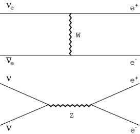
FIG. 1.: Feynman diagram for electron-positron pair creation through neutrino-antineutrino annihilation.

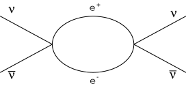
FIG. 2.: This is the diagrammatic representation of the polarization tensor used to calculate the rate of electron-positron pair production through neutrino-antineutrino annihilation. The imaginary part of this diagram is related to the rate of the process shown in figure 1.

II Basic formalism

Ultimately, we wish to calculate the rate at which neutrinos and antineutrinos interact with electrons and positrons in a strong magnetic field in matter through the processes shown in figure 1. Rather than calculate these rates directly through the use of the exact electron wave functions in the magnetic field, such as performed by Bezchastnov and Haensel [8] in their evaluation of the neutrino-electron scattering rate, we adopt an alternative approach suggested by the use of finite temperature field theory (FTFT). This theory has been pioneered by Weldon [10] and also applied by Gale and Kapusta [9] to calculate the rate at which electron-positron pairs are emitted from the fireball in heavy ion collisions.

According to Weldon [10] the decay and production rate of a boson with energy $E$ at temperature $T$ can be related to the imaginary part of the boson self energy $\Pi$ by

$$\Gamma(E)=-\frac{1}{E}\>{\rm Im}\{\Pi(E)\},$$ (1)

where $\Gamma=\Gamma_{d}-\Gamma_{i}$ is the difference of the forward rate of the boson decay $\Gamma_{d}$ and the rate of the inverse process $\Gamma_{i}$. The decay and production rates are related by the principle of detailed balance

$$\frac{\Gamma_{d}}{\Gamma_{i}}=e^{E/T},$$ (2)

from which we get

$$\Gamma_{d}(E)=-\frac{1}{E}\frac{1}{1-e^{-E/T}}\>{\rm Im}\{\Pi(E)\}.$$ (3)

Instead of considering the decay of a boson we will investigate first the case of neutrino-antineutrino annihilation to an electron-positron pair, $\nu\bar{\nu}\rightarrow e^{-}e^{+}$, in an electron-positron plasma at temperature $T_{e}$ and chemical potential $\mu_{e}$. The corresponding annihilation rate is given by equation (3), where the boson is replaced by the neutrino-antineutrino pair. To lowest order the self energy is now given by the diagram of figure 2 which contains an electron loop. The four momenta of the neutrino and antineutrino are denoted by $Q_{1}$ and $Q_{2}$ and of the electron and positron by $P_{1}$ and $P_{2}$, respectively. Here we use the notation $Q_{i}=(q_{i},{\bf q_{i}})$ with $q_{i}=|{\bf q_{i}}|$ and $P_{i}=(E_{i},{\bf p_{i}})$ with $E_{i}=\sqrt{p_{i}^{2}+m^{2}}$, where $m$ is the electron mass. Then in equation (3) $E=q_{1}+q_{2}$ holds and the self energy is given by a Lorentz tensor $\Pi_{\mu\nu}$.

Next we want to relate the annihilation rate to the differential rate $dR_{\nu\bar{\nu}}/{d^{3}q_{1}d^{3}q_{2}}$ describing the absorption of a neutrino-antineutrino pair with momenta ${\bf q_{1}}$ and ${\bf q_{2}}$ in the electron-positron plasma. Usually, this rate would be calculated from the matrix element ${\cal M}$ of figure 1 according to

$$\frac{dR_{\nu\bar{\nu}}}{d^{3}q_{1}d^{3}q_{2}} =\frac{1}{2q_{1}2q_{2}}\int\frac{d^{3}p_{1}}{2E_{1}(2\pi)^{3}}[1-n_{e^{+}}(E_{1})]\int\frac{d^{3}p_{2}}{2E_{2}(2\pi)^{3}}[1-n_{e^{-}}(E_{2})]$$ (5)

$$(2\pi)^{4}\delta^{4}(Q_{1}+Q_{2}-P_{1}-P_{2})\sum_{i}\langle|{\cal M}|^{2}\rangle,$$

where there is a sum over initial states and the Fermi distribution function for the electron is given by

$$n_{e^{-}}(E)=\frac{1}{e^{(E-\mu_{e})/T_{e}}+1}$$ (6)

and the one of the positron by replacing $\mu_{e}$ by $-\mu_{e}$ in equation (6). The distribution functions in equation (5) describe Pauli blocking of the produced electron and positron in the plasma.

Following Gale and Kapusta [9] the differential rate is obtained from the annihilation rate $\Gamma_{d}$ by taking into account the neutrino current

$$\frac{dR_{\nu\bar{\nu}}}{d^{3}q_{1}d^{3}q_{2}}=\frac{1}{2q_{1}2q_{2}}\frac{1}{1-e^{-E/T_{e}}}M^{\mu\nu}\>{\rm Im}\{\Pi_{\mu\nu}(Q_{1}+Q_{2})\}.$$ (7)

Here the leptonic tensor for the neutrinos is given by

$$M^{\mu\nu} = \sum_{s_{1}s_{2}}\bar{v}(q_{2})\gamma^{\mu}(1-\gamma_{5})u(q_{1})\bar{u}(q_{1})\gamma^{\nu}(1-\gamma_{5})v(q_{2})$$ (8)

$$= 8(Q_{2}^{\mu}Q_{1}^{\nu}+Q_{1}^{\mu}Q_{2}^{\nu}-(Q_{1}Q_{2})g^{\mu\nu}+iQ_{1\alpha}Q_{2\beta}\varepsilon^{\alpha\mu\beta\nu}),$$ (9)

where we have summed over the neutrino spins. This formula differs from the one for the dilepton production rate given in the appendix of ref. [9] by the absence of a photon propagator and a different structure of the leptonic tensor for massless neutrinos instead of electrons leading to the appearance of the antisymmetric tensor $\varepsilon^{\alpha\mu\beta\nu}$ in equation (9). Furthermore the two expressions differ by a factor $\exp{(E/T_{e})}$ according to (2) because we are considering a decay instead of a production rate.

The total rate for the production of electron-positron pairs from neutrino-antineutrino annihilation follows by integrating the differential forward rate, equation (7), over the neutrino distribution functions $f_{\nu,\bar{\nu}}(q_{i})$

$$R_{\nu\bar{\nu}}=\int\frac{d^{3}q_{1}}{(2\pi)^{3}}\int\frac{d^{3}q_{2}}{(2\pi)^{3}}[f_{\nu}(q_{1})f_{\bar{\nu}}(q_{2})-(1-f_{\nu}(q_{1}))(1-f_{\bar{\nu}}(q_{2}))e^{-E/T_{e}}]\>\frac{dR_{\nu\bar{\nu}}}{d^{3}q_{1}d^{3}q_{2}}.$$ (10)

Here we have included the back reaction $e^{-}e^{+}\rightarrow\nu\bar{\nu}$, which is described by the second term in the square brackets. It should be noted that our derivation of the rates at no time assumed that the neutrinos are in thermal equilibrium with the electron-positron plasma. For example, neutrinos that escape from the core of a supernova explosion may have a roughly thermal distribution with a temperature of $T_{\nu}\simeq 5$ MeV. After leaving the core these neutrinos will interact with the surrounding electron-positron plasma which has a typical temperature of about $T_{e}\simeq 1$ MeV. In this case the neutrino distribution functions in equation (10) are given by the equilibrium Fermi distributions, equation (6), where the temperature and the chemical potential are replaced by the corresponding values for the neutrinos escaping from the core, $T_{\nu}$ and $\mu_{\nu}$.

One may also determine the rate at which a neutrino scatters in a thermal plasma in a similar manner. The differential rate at which a neutrino (or antineutrino) scatters from an initial state $Q_{1}$ to a final state $Q_{2}$, is given simply by replacing $Q_{1}+Q_{2}$ by $Q_{1}-Q_{2}$ in ${\rm Im}\{\Pi_{\mu\nu}\}$ and $E=q_{1}+q_{2}$ by $q_{1}-q_{2}$ in equation (7). The total rate of scattering,$R_{\nu e^{\pm}}$, is then given by

$$R_{\nu e^{\pm}}=\int\frac{d^{3}q_{1}}{(2\pi)^{3}}\int\frac{d^{3}q_{2}}{(2\pi)^{3}}[f_{\nu}(q_{1})(1-f_{\nu}(q_{2}))-f_{\nu}(q_{2})(1-f_{\nu}(q_{1}))e^{-E/T_{e}}]\>\frac{dR_{\nu e^{\pm}}}{d^{3}q_{1}d^{3}q_{2}}$$ (11)

with

$$\frac{dR_{\nu e^{\pm}}}{d^{3}q_{1}d^{3}q_{2}}=\frac{1}{2q_{1}2q_{2}}\frac{1}{1-e^{-E/T_{e}}}M^{\mu\nu}\>{\rm Im}\{\Pi_{\mu\nu}(Q_{1}-Q_{2})\},$$ (12)

where $E=q_{1}-q_{2}$. Note that both the electron and positron scattering rates are included within the imaginary part of the polarisation tensor in equation (12). The strength of this method lies in the fact that the correct calculation of the imaginary part of the polarisation tensor leads the differential annihilation and scattering rates for all of the separate channels that are allowed within the plasma. Thus, if one includes the effect of the magnetic field in the polarisation tensor properly, all of the exotic processes which occur in a magnetic field are included in the rate calculations by default.

A The unmagnetized rate

To demonstrate that the two approaches, based either on the matrix element as in equation (5) or on the FTFT as in equation (7) are equivalent, we use equation (7) to calculate the rate of neutrino-antineutrino annihilation to electron positron pairs in an unmagnetized vacuum at zero temperature, and show that it reproduces the results of the calculation of the process using the matrix element method.

In the one-loop approximation the polarisation tensor in equation (7) is given by

$$\Pi^{\mu\nu}(K)=-{G_{F}^{2}\over 2}{\rm Tr}\int{d^{4}P\over(2\pi)^{4}}\gamma^{\mu}(c_{V}-c_{A}\gamma_{5})G(P)\gamma^{\nu}(c_{V}-c_{A}\gamma_{5})G(P-K),$$ (13)

where $G_{F}$ is the Fermi constant, $G(P)$ is an electron propagator, and

$$c_{V}=\pm{1\over 2}+2\sin^{2}\theta_{W},\qquad c_{A}=\pm{1\over 2}$$ (14)

with $\theta_{W}$ the Weinberg angle, and the plus sign corresponding to electron neutrinos, and the minus sign to muon and tau neutrinos. This tensor has been formulated in the limit that the neutrino energies are small compared to the $W$ mass, which will always be justified in practice. This allows the use of effective Fermi 4-vertices in the processes shown in figure 1 and 2. The polarization tensor in equation (13) may be decomposed into vector-vector, axial-vector, and axial-axial parts through

$$\Pi^{\mu\nu}=c_{V}^{2}\alpha^{\mu\nu}+2c_{V}c_{A}\alpha^{\mu\nu}_{5}+c_{A}^{2}\alpha^{\mu\nu}_{55}$$ (15)

with

$$\alpha^{\mu\nu}=-{G_{F}^{2}\over 2}{\rm Tr}\int{d^{4}P\over(2\pi)^{4}}\gamma^{\mu}G(P)\gamma^{\nu}G(P-K),$$ (16)

$$\alpha^{\mu\nu}_{5}={G_{F}^{2}\over 2}{\rm Tr}\int{d^{4}P\over(2\pi)^{4}}{1\over 2}\left[\gamma^{\mu}\gamma_{5}G(P)\gamma^{\nu}G(P-K)+\gamma^{\mu}G(P)\gamma^{\nu}\gamma_{5}G(P-K)\right],$$ (17)

and

$$\alpha^{\mu\nu}_{55}=-{G_{F}^{2}\over 2}{\rm Tr}\int{d^{4}P\over(2\pi)^{4}}\gamma^{\mu}\gamma_{5}G(P)\gamma^{\nu}\gamma_{5}G(P-K).$$ (18)

In this section we will neglect matter contributions to the rate, i.e., we set $T_{e}=0$ in equation (7), set the distribution function to zero and use only the vacuum part of the polarization tensor, equation (13). This corresponds to neglecting the effects of Pauli blocking on the final state particles in equation (5). Inserting only the vacuum part of the electron propagators, the vacuum part of the polarization tensor, equation (13), may be written

$$\Pi^{\mu\nu}(K)=-{G_{F}^{2}\over 2}{\rm Tr}\int{d^{4}P\over(2\pi)^{4}}{\gamma^{\mu}(c_{V}-c_{A}\gamma_{5})(/\!\!\!\!P+m)\gamma^{\nu}(c_{V}-c_{A}\gamma_{5})(/\!\!\!\!P-/\!\!\!\!K+m)\over\left[P^{2}-m^{2}+i0\right]\left[(P-K)^{2}-m^{2}+i0\right]}.$$ (19)

Note that the real part of this tensor must be renormalized due to the singularities in the denominator of the integrand, but the imaginary part is finite.

The imaginary part of $\Pi^{\mu\nu}$ (actually, the anti-hermitian part) is related to its discontinuity across a branch cut. The branch cut is related to poles that appear above the pair creation threshold, $K^{2}=4m^{2}$, and it lies along the positive $K^{2}$ axis from $4m^{2}$ to infinity. One has

$${\rm Im}\{\Pi^{\mu\nu}(K)\}=-{G_{F}^{2}\over 32\pi^{2}}I^{\mu\nu}$$ (20)

with

$$I^{\mu\nu} = \int d^{4}P\>{\rm Tr}\left[\gamma^{\mu}(c_{V}-c_{A}\gamma_{5})(/\!\!\!\!P+m)\gamma^{\nu}(c_{V}-c_{A}\gamma_{5})(/\!\!\!\!P-/\!\!\!\!K+m)\right]$$ (22)

$$\qquad\times\delta(P^{2}-m^{2})\,\delta((P-K)^{2}-m^{2}).$$

Inserting a delta function into equation (22) and relabelling $P\rightarrow P_{1}$, leads to

$$I^{\mu\nu} = -\int d^{4}P_{1}\int d^{4}P_{2}\>{\rm Tr}\left[\gamma^{\mu}(c_{V}-c_{A}\gamma_{5})(/\!\!\!\!P_{1}+m)\gamma^{\nu}(c_{V}-c_{A}\gamma_{5})(/\!\!\!\!P_{2}-m)\right]$$ (24)

$$\qquad\times\delta(P_{1}^{2}-m^{2})\,\delta(P_{2}^{2}-m^{2})\delta^{4}(P_{2}+P_{1}-K).$$

The trace in the integrand of equation (24) may be recognized as proportional to the electron leptonic tensor, $L^{\mu\nu}$, and the rate of pair production, equation (7), is then given by

$${dR\over d^{3}q_{1}d^{3}q_{2}}={G_{F}^{2}\over 2}\int{d^{3}p_{1}\over(2\pi)^{3}}\int{d^{3}p_{2}\over(2\pi)^{3}}{L_{\mu\nu}M^{\mu\nu}\over 2E_{1}\,2E_{2}\,2q_{1}\,2q_{2}}(2\pi)^{4}\,\delta^{4}(P_{1}+P_{2}-Q_{1}-Q_{2}),$$ (25)

where

$$\int d^{4}P_{i}\,\delta(P_{i}^{2}-m^{2})=\int{d^{3}p_{i}\over E_{i}}$$ (26)

has been used.

Equation (25) is identical to the rate, equation (4), directly calculated for the process shown in figure 1 by electroweak theory, using $L_{\mu\nu}M^{\mu\nu}=\sum_{i}\langle|{\cal M}|^{2}\rangle$. Thus we have shown that the procedure outlined above is identical to the standard method of calculating rates.

For later reference, the rate at which the annihilation process proceeds in the absence of a magnetic field at zero temperature and in the limit of a vanishing electron mass, $m=0$, is given by

$${dR\over d^{3}q_{1}d^{3}q_{2}}={2G_{F}^{2}(c_{V}^{2}+c_{A}^{2})\over 3\pi}q_{1}^{2}q_{2}^{2}(1-\cos\Theta)^{2},$$ (27)

where $\Theta$ is the angle between the neutrino and antineutrino.

III Strong magnetic fields

We may now make a significant generalization of our theory, which justifies its introduction. The essential point is that the polarization tensor used in equation (7) contains all the information about the electronic part of the process, without reference to the presence or lack of a medium, or the presence or lack of a magnetic field. All that is required to calculate the correct rate is the appropriate polarization tensor for the given plasma. To determine the rate of neutrino-electron processes in a strongly magnetized plasma, one must use the polarization tensor for a strongly magnetized plasma. Thankfully, for our purposes, the polarization tensors in a strong magnetic field are well known, the vector-vector part was calculated in the form used here by Melrose and coworkers [11], the vector-axial part was calculated by Kennett and Melrose [12], and the axial-axial part may be calculated in a manner directly analogous to both.

The polarization tensor is calculated in [11] and [12] using a vertex formulation of the coupling between an electron in a magnetic field and an external 4 current. The various parts of the polarization tensor can be expressed in terms of the vector vertex function $[\Gamma^{\epsilon^{\prime}\epsilon}_{q^{\prime}q}(K)]^{\mu}$, and the axial vertex function, $\ {}_{5}[\Gamma^{\epsilon^{\prime}\epsilon}_{q^{\prime}q}(K)]^{\mu}$, where $q^{\prime}$ and $q$ denote the quantum numbers of the particles on either side of the interaction ($p_{\parallel}$, momentum, $\sigma$, spin, $n$, Landau orbital), and $\epsilon$ and $\epsilon^{\prime}$ denote the nature of the particles, with a plus sign for electrons (the particles) and a minus sign for the positrons (the antiparticles). The various components of the polarization tensor may be written,

$$\alpha^{\mu\nu}(K) = -{G_{F}^{2}eB\over 4\pi}\sum_{n^{\prime},n=0}^{\infty}\sum_{\epsilon^{\prime},\epsilon=\pm 1}$$ (29)

$$\qquad\times\int{dp_{\parallel}\over 2\pi}{\left\{{1\over 2}(\epsilon^{\prime}-\epsilon)+\epsilon n^{\epsilon}_{q}-\epsilon^{\prime}n^{\epsilon^{\prime}}_{q^{\prime}}\right\}\over\omega-\epsilon\varepsilon_{q}+\epsilon^{\prime}\varepsilon_{q^{\prime}}+i0}T^{\mu\nu}_{\epsilon^{\prime}\epsilon},$$

$$\alpha^{\mu\nu}_{5}(K) = {G_{F}^{2}eB\over 4\pi}\sum_{n^{\prime},n=0}^{\infty}\sum_{\epsilon^{\prime},\epsilon=\pm 1}$$ (31)

$$\qquad\times\int{dp_{\parallel}\over 2\pi}{\left\{{1\over 2}(\epsilon^{\prime}-\epsilon)+\epsilon n^{\epsilon}_{q}-\epsilon^{\prime}n^{\epsilon^{\prime}}_{q^{\prime}}\right\}\over\omega-\epsilon\varepsilon_{q}+\epsilon^{\prime}\varepsilon_{q^{\prime}}+i0}\,_{5}T^{\mu\nu}_{\epsilon^{\prime}\epsilon},$$

$$\alpha^{\mu\nu}_{55}(K) = -{G_{F}^{2}eB\over 4\pi}\sum_{n^{\prime},n=0}^{\infty}\sum_{\epsilon^{\prime},\epsilon=\pm 1}$$ (33)

$$\qquad\times\int{dp_{\parallel}\over 2\pi}{\left\{{1\over 2}(\epsilon^{\prime}-\epsilon)+\epsilon n^{\epsilon}_{q}-\epsilon^{\prime}n^{\epsilon^{\prime}}_{q^{\prime}}\right\}\over\omega-\epsilon\varepsilon_{q}+\epsilon^{\prime}\varepsilon_{q^{\prime}}+i0}\,_{55}T^{\mu\nu}_{\epsilon^{\prime}\epsilon}$$

with

$$T^{\mu\nu}_{\epsilon^{\prime}\epsilon}=\sum_{\sigma^{\prime},\sigma=\pm 1}[\Gamma^{\epsilon^{\prime}\epsilon}_{q^{\prime}q}({\bf k})]^{\mu}[\Gamma^{\epsilon^{\prime}\epsilon}_{q^{\prime}q}({\bf k})]^{\nu*},$$ (34)

$$\,{}_{5}T^{\mu\nu}_{\epsilon^{\prime}\epsilon}=\sum_{\sigma^{\prime},\sigma=\pm 1}{1\over 2}\left\{\,{}_{5}[\Gamma^{\epsilon^{\prime}\epsilon}_{q^{\prime}q}({\bf k})]^{\mu}[\Gamma^{\epsilon^{\prime}\epsilon}_{q^{\prime}q}({\bf k})]^{\nu*}+[\Gamma^{\epsilon^{\prime}\epsilon}_{q^{\prime}q}({\bf k})]^{\mu}\,_{5}[\Gamma^{\epsilon^{\prime}\epsilon}_{q^{\prime}q}({\bf k})]^{\nu*}\right\},$$ (35)

$$\,{}_{55}T^{\mu\nu}_{\epsilon^{\prime}\epsilon}=\sum_{\sigma^{\prime},\sigma=\pm 1}\,{}_{5}[\Gamma^{\epsilon^{\prime}\epsilon}_{q^{\prime}q}({\bf k})]^{\mu}\,_{5}[\Gamma^{\epsilon^{\prime}\epsilon}_{q^{\prime}q}({\bf k})]^{\nu*},$$ (36)

and where $K=(\omega,{\bf k})$, $n^{\epsilon}_{q}$ are the electron distribution functions, and $\varepsilon_{q}$ denotes the energy of the particle in the magnetic field,

$$\varepsilon_{q}\equiv\varepsilon(p_{\parallel},n)=\left(m^{2}+p_{\parallel}^{2}+2neB\right)^{1/2}.$$ (37)

Implicit throughout equations (29) to (36) is the relation $\epsilon^{\prime}p_{\parallel}^{\prime}=\epsilon p_{\parallel}-k_{\parallel}$. Note also that we are using natural units with all physical quantities scaled against the electron mass.

The polarization tensors given in equations (29) to (33) contain the contributions from both the vacuum polarization and the electrons and positrons in the plasma. The vacuum part is given by the term ${1\over 2}(\epsilon^{\prime}-\epsilon)$ in the numerator of the integrand. The real part of this term is divergent and must be renormalized. We are concerned here only with the imaginary part, which is finite. Hence, we perform no renormalization here. The electrons and positrons of the plasma contribute to the polarization tensor through the distribution functions (more properly, the occupation numbers) $n^{\epsilon}_{q}$, which in a magnetized thermal medium are given by the Fermi distributions

$$n^{\epsilon}_{q}\equiv n^{\epsilon}(p_{\parallel},n)=\frac{1}{e^{(\varepsilon(p_{\parallel},n)-\epsilon\mu_{e})/T_{e}}+1}.$$ (38)

The general form of the magnetic vertex functions are given in [12], and a general discussion of the properties of the vector part may be found in [11]. The components of the vertex functions are

$$[\Gamma^{\epsilon\epsilon^{\prime}}_{q^{\prime}q}({\bf k})]^{0} = C_{q^{\prime}}C_{q}[\delta_{\sigma^{\prime},\sigma}(\delta_{\epsilon^{\prime},\epsilon}{\cal B}+\sigma\delta_{\epsilon^{\prime},-\epsilon}{\cal A})(J^{l}_{l^{\prime}-l}+\rho_{n^{\prime}}\rho_{n}J^{l+\sigma}_{l^{\prime}-l})$$ (40)

$$-\epsilon\delta_{\sigma^{\prime},-\sigma}(\sigma\delta_{\epsilon^{\prime},\epsilon}{\cal A}-\delta_{\epsilon^{\prime},-\epsilon}{\cal B})(-\rho_{n}J^{l+\sigma}_{l^{\prime}-l-\sigma}+\rho_{n^{\prime}}J^{l}_{l^{\prime}-l-\sigma})],$$

$$[\Gamma^{\epsilon\epsilon^{\prime}}_{q^{\prime}q}({\bf k})]^{1} = C_{q^{\prime}}C_{q}[\delta_{\sigma^{\prime},\sigma}\epsilon(\delta_{\epsilon^{\prime},\epsilon}{\cal D}+\sigma\delta_{\epsilon^{\prime},-\epsilon}{\cal C})(-\rho_{n}J^{l+\sigma}_{l^{\prime}-l-\sigma}-\rho_{n^{\prime}}J^{l}_{l^{\prime}-l+\sigma})$$ (42)

$$-\delta_{\sigma^{\prime},-\sigma}(\sigma\delta_{\epsilon^{\prime},\epsilon}{\cal C}-\delta_{\epsilon^{\prime},-\epsilon}{\cal D})(J^{l}_{l^{\prime}-l}-\rho_{n^{\prime}}\rho_{n}J^{l+\sigma}_{l^{\prime}-l-2\sigma})],$$

$$[\Gamma^{\epsilon\epsilon^{\prime}}_{q^{\prime}q}({\bf k})]^{2} = iC_{q^{\prime}}C_{q}[\delta_{\sigma^{\prime},\sigma}\epsilon(\sigma\delta_{\epsilon^{\prime},\epsilon}{\cal D}+\delta_{\epsilon^{\prime},-\epsilon}{\cal C})(\rho_{n}J^{l+\sigma}_{l^{\prime}-l-\sigma}-\rho_{n^{\prime}}J^{l}_{l^{\prime}-l+\sigma})$$ (44)

$$-\delta_{\sigma^{\prime},-\sigma}(\delta_{\epsilon^{\prime},\epsilon}{\cal C}-\sigma\delta_{\epsilon^{\prime},-\epsilon}{\cal D})(J^{l}_{l^{\prime}-l}+\rho_{n^{\prime}}\rho_{n}J^{l+\sigma}_{l^{\prime}-l-2\sigma})],$$

$$[\Gamma^{\epsilon\epsilon^{\prime}}_{q^{\prime}q}({\bf k})]^{3} = C_{q^{\prime}}C_{q}[\delta_{\sigma^{\prime},\sigma}(\delta_{\epsilon^{\prime},\epsilon}{\cal A}+\sigma\delta_{\epsilon^{\prime},-\epsilon}{\cal B})(J^{l}_{l^{\prime}-l}+\rho_{n^{\prime}}\rho_{n}J^{l+\sigma}_{l^{\prime}-l})$$ (46)

$$-\epsilon\delta_{\sigma^{\prime},-\sigma}(\sigma\delta_{\epsilon^{\prime},\epsilon}{\cal B}-\delta_{\epsilon^{\prime},-\epsilon}{\cal A})(-\rho_{n}J^{l+\sigma}_{l^{\prime}-l-\sigma}+\rho_{n^{\prime}}J^{l}_{l^{\prime}-l-\sigma})],$$

and

$$\,{}_{5}[\Gamma^{\epsilon\epsilon^{\prime}}_{q^{\prime}q}({\bf k})]^{0} = C_{q^{\prime}}C_{q}[\delta_{\sigma^{\prime},\sigma}(\sigma\delta_{\epsilon^{\prime},\epsilon}{\cal A}+\delta_{\epsilon^{\prime},-\epsilon}{\cal B})(J^{l}_{l^{\prime}-l}-\rho_{n^{\prime}}\rho_{n}J^{l+\sigma}_{l^{\prime}-l})$$ (48)

$$-\epsilon\delta_{\sigma^{\prime},-\sigma}(-\delta_{\epsilon^{\prime},\epsilon}{\cal B}+\sigma\delta_{\epsilon^{\prime},-\epsilon}{\cal A})(-\rho_{n}J^{l+\sigma}_{l^{\prime}-l-\sigma}-\rho_{n^{\prime}}J^{l}_{l^{\prime}-l-\sigma})],$$

$$\,{}_{5}[\Gamma^{\epsilon\epsilon^{\prime}}_{q^{\prime}q}({\bf k})]^{1} = C_{q^{\prime}}C_{q}[\delta_{\sigma^{\prime},\sigma}\epsilon(\sigma\delta_{\epsilon^{\prime},\epsilon}{\cal C}+\delta_{\epsilon^{\prime},-\epsilon}{\cal D})(-\rho_{n}J^{l+\sigma}_{l^{\prime}-l-\sigma}+\rho_{n^{\prime}}J^{l}_{l^{\prime}-l+\sigma})$$ (50)

$$-\delta_{\sigma^{\prime},-\sigma}(-\delta_{\epsilon^{\prime},\epsilon}{\cal D}+\sigma\delta_{\epsilon^{\prime},-\epsilon}{\cal C})(J^{l}_{l^{\prime}-l}+\rho_{n^{\prime}}\rho_{n}J^{l+\sigma}_{l^{\prime}-l-2\sigma})],$$

$$\,{}_{5}[\Gamma^{\epsilon\epsilon^{\prime}}_{q^{\prime}q}({\bf k})]^{2} = iC_{q^{\prime}}C_{q}[\delta_{\sigma^{\prime},\sigma}\epsilon(\delta_{\epsilon^{\prime},\epsilon}{\cal C}+\sigma\delta_{\epsilon^{\prime},-\epsilon}{\cal D})(\rho_{n}J^{l+\sigma}_{l^{\prime}-l-\sigma}+\rho_{n^{\prime}}J^{l}_{l^{\prime}-l+\sigma})$$ (52)

$$-\delta_{\sigma^{\prime},-\sigma}(-\sigma\delta_{\epsilon^{\prime},\epsilon}{\cal D}+\delta_{\epsilon^{\prime},-\epsilon}{\cal C})(J^{l}_{l^{\prime}-l}-\rho_{n^{\prime}}\rho_{n}J^{l+\sigma}_{l^{\prime}-l-2\sigma})],$$

$$\,{}_{5}[\Gamma^{\epsilon\epsilon^{\prime}}_{q^{\prime}q}({\bf k})]^{3} = C_{q^{\prime}}C_{q}[\delta_{\sigma^{\prime},\sigma}(\sigma\delta_{\epsilon^{\prime},\epsilon}{\cal B}+\delta_{\epsilon^{\prime},-\epsilon}{\cal A})(J^{l}_{l^{\prime}-l}-\rho_{n^{\prime}}\rho_{n}J^{l+\sigma}_{l^{\prime}-l})$$ (54)

$$-\delta_{\sigma^{\prime},-\sigma}\epsilon(-\delta_{\epsilon^{\prime},\epsilon}{\cal A}+\sigma\delta_{\epsilon^{\prime},-\epsilon}{\cal B})(-\rho_{n}J^{l+\sigma}_{l^{\prime}-l-\sigma}-\rho_{n^{\prime}}J^{l}_{l^{\prime}-l-\sigma})],$$

where $l=n-{1\over 2}(1+\sigma)$ is an orbital quantum number, and

$$C_{q}\equiv\left({(\varepsilon_{q}+\varepsilon_{q}^{0})(\varepsilon_{q}^{0}+m)\over 4\varepsilon_{q}^{0}\varepsilon_{q}}\right)^{1/2},$$ (55)

$$\rho_{\parallel}\equiv p_{\parallel}/(\varepsilon_{q}+\varepsilon_{q}^{0}),\qquad\rho_{n}\equiv p_{n}/(\varepsilon_{q}^{0}+m),$$ (56)

$${\cal A}=\rho_{\parallel}^{\prime}+\rho_{\parallel},\qquad{\cal B}=1+\rho_{\parallel}^{\prime}\rho_{\parallel},$$ (57)

$${\cal C}=\rho_{\parallel}^{\prime}-\rho_{\parallel},\qquad{\cal D}=1-\rho_{\parallel}^{\prime}\rho_{\parallel},$$ (58)

and $p_{n}=\sqrt{2nB}$, $\varepsilon_{q}^{0}\equiv\varepsilon(0,n)$, and the primed versions of the same quantities have unprimed variables replaced by primed variables. Note again that $\epsilon^{\prime}p_{\parallel}^{\prime}=\epsilon p_{\parallel}-k_{\parallel}$ is implicit throughout.

The functions $J^{n}_{v}(k_{\perp}^{2}/2B)$ in equations (40) to (54) (the argument is suppressed) are generalized functions related to the Laguerre polynomials and defined by

$$J^{n}_{v}(x)=\left[{n!\over(n+v)!}\right]^{1/2}\exp(-x/2)x^{v/2}L^{v}_{n}(x)=(-1)^{v}J^{n+v}_{-v}(x),$$ (59)

where $L^{v}_{n}(x)$ are associated Laguerre polynomials. One may write explicitly

$$J^{n}_{v}(x)=\exp(-x/2)x^{v/2}\sum_{m=0}^{n}(-1)^{m}{\left[n!(n+v)!\right]^{1/2}\over(v+m)!(n-m)!m!}x^{m}.$$ (60)

Note that $J^{n}_{v}(x)=0$ if $n<0$ or $v<-n$. A summary of the properties of the $J$ functions may be found in [11].

A Annihilation rate

We now use the imaginary parts of equations (29) to (33) to determine the rate at which a neutrino annihilates on an antineutrino in a strongly magnetized electron-positron plasma. The imaginary parts of these integrals come from the poles in the denominators of the integrands, where $\omega-\epsilon\varepsilon_{q}+\epsilon^{\prime}\varepsilon_{q^{\prime}}=0$. The contribution of these poles may be calculated through the Plemelj formula

$${1\over\omega-\omega_{0}}={\cal P}{1\over\omega-\omega_{0}}-i\pi\delta(\omega-\omega_{0}),$$ (61)

where ${\cal P}$ denotes the principle value. The integral over the delta-function introduced into equations (29) to (33) by the Plemelj formula may be done explicitly by determining the positions of the poles of the integrand. For $\omega>0$, which is the case for neutrino-antineutrino annihilation, the denominators of equations (29) to (33) only have zeros if $\epsilon=1$, $\epsilon^{\prime}=-1$, (pair creation), $\epsilon=-1$, $\epsilon^{\prime}=-1$ (neutrino pair absorption on a positron), and $\epsilon=1$, $\epsilon^{\prime}=1$ (neutrino pair absorption on an electron). Each of these processes occurs in a different region of the phase space, determined by the existence of the roots of the energy conservation equation $\omega-\epsilon\varepsilon_{q}+\epsilon^{\prime}\varepsilon_{q^{\prime}}=0$. Writing $\delta=\omega^{2}-k_{\parallel}^{2}$, this equation has general solutions of the form

$$p_{\parallel}=\pm{k_{\parallel}\over 2}\xi\pm{\omega\over 2}\Delta^{1/2}$$ (62)

with

$$\xi=1+{2(n-n^{\prime})B\over\delta},$$ (63)

and

$$\Delta=\xi^{2}-{4(1+2nB)\over\delta}.$$ (64)

The roots given by equation (62) are real if $\Delta>0$, which is true if and only if

$$0<\delta<\left[\sqrt{1+2n^{\prime}B}-\sqrt{1+2nB}\right]^{2},$$ (65)

which corresponds to a pair absorption on an electron or positron, and

$$\delta>\left[\sqrt{1+2n^{\prime}B}+\sqrt{1+2nB}\right]^{2},$$ (66)

which corresponds to an electron positron pair creation. Note that for two annihilating neutrinos one has $\delta=\omega^{2}-k_{\parallel}^{2}>0$.

The contributions of the vector-vector, axial-vector and axial-axial parts of the rates may be separated out through

$$\frac{dR_{\nu\bar{\nu}}}{d^{3}q_{1}d^{3}q_{2}}={1\over 2q_{1}2q_{2}}\frac{1}{1-e^{-E/T_{e}}}M_{\mu\nu}{\rm Im}\{c_{V}^{2}\alpha^{\mu\nu}(K)+2c_{V}c_{A}\,\alpha^{\mu\nu}_{5}(K)+c_{A}^{2}\,\alpha^{\mu\nu}_{55}(K)\}$$ (67)

with $K=Q_{1}+Q_{2}$. Each of the polarization tensor components in equation (67) contains a sum over two sets of Landau levels evaluated at the root of the denominator, and a sum over the $\epsilon$ and $\epsilon^{\prime}$, which denote the type of particles which are interacting. Here, we divide the rate into the three contributing combinations of $\epsilon$ and $\epsilon^{\prime}$, corresponding to three different physical processes.

1 Neutrino pair creation

If equation (66) holds, and $\epsilon=1$, $\epsilon^{\prime}=-1$, the poles in the integrand of the polarization tensor components correspond to the physical process of neutrino-antineutrino annihilation to form an electron-positron pair, $\nu\bar{\nu}\leftrightarrow e^{+}e^{-}$. Letting $X$ stand for a blank, 5, or 55, the imaginary part of the polarization tensor components may be written

$${\rm Im}\{\alpha^{\mu\nu}_{X}(K)\} = {G_{F}^{2}eB\over 4\pi}\sum_{n,n^{\prime}=0}^{\infty}{\varepsilon_{q}\varepsilon_{q^{\prime}}\over|p_{\parallel}\varepsilon_{q^{\prime}}-p_{\parallel}^{\prime}\varepsilon_{q}|}\times$$ (69)

$$\left.\,{}_{X}T^{\mu\nu}_{-+}(-1+n_{e^{-}}(p_{\parallel},n)+n_{e^{+}}(p_{\parallel}^{\prime},n^{\prime}))\right|_{p_{\parallel}:\omega-\varepsilon_{q}-\varepsilon_{q^{\prime}}=0}$$

with $p_{\parallel}^{\prime}=-p_{\parallel}+k_{\parallel}$. This equation is combined with equation (67) and equation (10) to obtain the net rate of annihilation to neutrino antineutrino pairs to electron positron pairs. The sum in equation (69) is evaluated at the parallel momenta for which the resonance condition is satisfied

$$p_{\parallel}={k_{\parallel}\over 2}\xi\pm{\omega\over 2}\Delta^{1/2},$$ (70)

$$p_{\parallel}^{\prime}={k_{\parallel}\over 2}\xi\mp{\omega\over 2}\Delta^{1/2}.$$ (71)

Equation (69) should be evaluated at both of these roots, and the sum over the Landau orbitals is limited to $n$ and $n^{\prime}$ such that $\sqrt{1+2nB}+\sqrt{1+2n^{\prime}B}<\sqrt{\omega^{2}-k_{\parallel}^{2}}$.

The form taken by the blocking factors in equation (69) is due to the fact that the imaginary part of the polarization tensor is related to the difference of the forward and reverse rates [10].

2 Gyromagnetic absorption on positrons

If condition (65) holds and if $n^{\prime}>n$, with $\epsilon=-1$, and $\epsilon^{\prime}=-1$, the neutrino-antineutrino pair may be absorbed on a positron, $\nu\bar{\nu}e^{+}\leftrightarrow e^{+}$, a process which is forbidden in the absence of a strong magnetic field. The contribution to the imaginary part of the polarization tensor due to the root corresponding to this process may be written

$${\rm Im}\{\alpha^{\mu\nu}_{X}(K)\} = {G_{F}^{2}eB\over 4\pi}\sum_{n,n^{\prime}=0}^{\infty}{\varepsilon_{q}\varepsilon_{q^{\prime}}\over|p_{\parallel}\varepsilon_{q^{\prime}}-p_{\parallel}^{\prime}\varepsilon_{q}|}\times$$ (73)

$$\left.\,{}_{X}T^{\mu\nu}_{--}(-n_{e^{+}}(p_{\parallel},n)+n_{e^{+}}(p_{\parallel}^{\prime},n^{\prime}))\right|_{p_{\parallel}:\omega+\varepsilon_{q}-\varepsilon_{q^{\prime}}=0}$$

with $p_{\parallel}^{\prime}=p_{\parallel}+k_{\parallel}$. The sum is evaluated for this process at parallel momenta

$$p_{\parallel}=-{k_{\parallel}\over 2}\xi\pm{\omega\over 2}\Delta^{1/2},$$ (74)

$$p_{\parallel}^{\prime}={k_{\parallel}\over 2}\xi\pm{\omega\over 2}\Delta^{1/2}.$$ (75)

3 Gyromagnetic absorption on electrons

On the other hand, if condition (65) holds and if $n>n^{\prime}$, and $\epsilon=1$ and $\epsilon^{\prime}=1$, the neutrino-antineutrino pair may be absorbed on an electron, $\nu\bar{\nu}e^{-}\leftrightarrow e^{-}$, a process which is also forbidden in the absence of a strong magnetic field. The contribution to the imaginary part of the polarization tensor due to the root corresponding to this process may be written

$${\rm Im}\{\alpha^{\mu\nu}_{X}(K)\} = {G_{F}^{2}eB\over 4\pi}\sum_{n,n^{\prime}=0}^{\infty}{\varepsilon_{q}\varepsilon_{q^{\prime}}\over|p_{\parallel}\varepsilon_{q^{\prime}}-p_{\parallel}^{\prime}\varepsilon_{q}|}\times$$ (77)

$$\left.\,{}_{X}T^{\mu\nu}_{++}(n_{e^{-}}(p_{\parallel},n)-n_{e^{-}}(p_{\parallel}^{\prime},n^{\prime}))\right|_{p_{\parallel}:\omega-\varepsilon_{q}+\varepsilon_{q^{\prime}}=0}$$

with $p_{\parallel}^{\prime}=p_{\parallel}-k_{\parallel}$. The sum in equation (77) should be evaluated at the roots

$$p_{\parallel}={k_{\parallel}\over 2}\xi\pm{\omega\over 2}\Delta^{1/2},$$ (78)

$$p_{\parallel}^{\prime}=-{k_{\parallel}\over 2}\xi\pm{\omega\over 2}\Delta^{1/2}.$$ (79)

For the gyromagnetic absorption processes, the limits on the sums over the Landau levels enumerated by $n$ and $n^{\prime}$ are given by $\left|\sqrt{1+2nB}-\sqrt{1+2n^{\prime}B}\right|>\sqrt{\omega^{2}-k_{\parallel}^{2}}$. There is no upper limit on either $n$ or $n^{\prime}$ implied by this relation. Instead, the upper limit on the Landau level is constrained by the fact that one of the distribution functions in equations (73) and (77) must be non-zero for there to be a rate, and these distribution functions are sampled at the resonant momenta given above, which grow with increasing Landau number.

B Scattering rate

A similar procedure may be used to calculate the rate of scattering of a neutrino or antineutrino off a thermal pair plasma in a strong magnetic field. In this case, the frequency of the disturbance in the field is given by $\omega=q_{1}-q_{2}$, which may be negative or positive. Hence, there are four contributions to the scattering rate, whereas there are only three contributions to the annihilation rate. The processes correspond to $\epsilon=1$,$\epsilon^{\prime}=-1$, pair creation by a neutrino, $\epsilon=1$,$\epsilon^{\prime}=-1$ pair absorption by a neutrino, $\epsilon=-1$,$\epsilon^{\prime}=-1$, neutrino positron scattering, and $\epsilon=1$,$\epsilon^{\prime}=1$ neutrino electron scattering. The rates of these processes are given by equation (11) with

$$\frac{dR_{\nu e^{\pm}}}{d^{3}q_{1}d^{3}q_{2}}={1\over 2q_{1}2q_{2}}\frac{1}{1-e^{-E/T_{e}}}M_{\mu\nu}{\rm Im}\{c_{V}^{2}\alpha^{\mu\nu}(K)+2c_{V}c_{A}\,\alpha^{\mu\nu}_{5}(K)+c_{A}^{2}\,\alpha^{\mu\nu}_{55}(K)\}$$ (80)

and with $K=Q_{1}-Q_{2}$. Again, the scattering and absorption processes occur in different regions of the phase space, with the conditions

$$\delta=\omega^{2}-k_{\parallel}^{2}<\left[\sqrt{1+2n^{\prime}B}-\sqrt{1+2nB}\right]^{2},$$ (81)

which corresponds to neutrino scattering off electrons and positrons, and

$$\delta>\left[\sqrt{1+2n^{\prime}B}+\sqrt{1+2nB}\right]^{2},$$ (82)

which corresponds to electron positron pair creation and absorption on neutrinos.

1 Electron-positron pair creation and absorption

The contribution of the pair creation and absorption processes to the total neutrino scattering rate, $\nu e^{+}e^{-}\leftrightarrow\nu$, appears in two parts, for opposite signs of the energy transfer, $\omega$. For $\omega=q_{1}-q_{2}>0$, one has a contribution for $\epsilon=1$, $\epsilon^{\prime}=-1$ if $\delta>\left[\sqrt{1+2nB}+\sqrt{1+2n^{\prime}B}\right]^{2}$. This contribution is given by

$${\rm Im}\{\alpha^{\mu\nu}_{X}(K)\} = {G_{F}^{2}eB\over 4\pi}\sum_{n,n^{\prime}=0}^{\infty}{\varepsilon_{q}\varepsilon_{q^{\prime}}\over|p_{\parallel}\varepsilon_{q^{\prime}}-p_{\parallel}^{\prime}\varepsilon_{q}|}\times$$ (84)

$$\left.\,{}_{X}T^{\mu\nu}_{+-}(-1+n_{e^{-}}(p_{\parallel},n)+n_{e^{+}}(p_{\parallel}^{\prime},n^{\prime}))\right|_{p_{\parallel}:\omega-\varepsilon_{q}-\varepsilon_{q^{\prime}}=0}$$

with $p_{\parallel}^{\prime}=-p_{\parallel}+k_{\parallel}$. Equation (84) should be evaluated at both the roots given by,

$$p_{\parallel}={k_{\parallel}\over 2}\xi\pm{\omega\over 2}\Delta^{1/2},$$ (85)

$$p_{\parallel}^{\prime}={k_{\parallel}\over 2}\xi\mp{\omega\over 2}\Delta^{1/2}.$$ (86)

For negative energy transfer, $\omega=q_{1}-q_{2}<0$, one has a contribution for $\epsilon=-1$, $\epsilon^{\prime}=1$ if $\delta>\left[\sqrt{1+2nB}+\sqrt{1+2n^{\prime}B}\right]^{2}$. This contribution is given by

$${\rm Im}\{\alpha^{\mu\nu}_{X}(K)\} = {G_{F}^{2}eB\over 4\pi}\sum_{n,n^{\prime}=0}^{\infty}{\varepsilon_{q}\varepsilon_{q^{\prime}}\over|p_{\parallel}\varepsilon_{q^{\prime}}-p_{\parallel}^{\prime}\varepsilon_{q}|}\times$$ (88)

$$\left.\,{}_{X}T^{\mu\nu}_{-+}(1-n_{e^{+}}(p_{\parallel},n)-n_{e^{-}}(p_{\parallel}^{\prime},n^{\prime}))\right|_{p_{\parallel}:\omega+\varepsilon_{q}+\varepsilon_{q^{\prime}}=0}$$

with $p_{\parallel}^{\prime}=-p_{\parallel}-k_{\parallel}$. Equation (88) should be evaluated at both the roots given by,

$$p_{\parallel}=-{k_{\parallel}\over 2}\xi\pm{\omega\over 2}\Delta^{1/2},$$ (89)

$$p_{\parallel}^{\prime}=-{k_{\parallel}\over 2}\xi\mp{\omega\over 2}\Delta^{1/2}.$$ (90)

2 Neutrino-electron scattering

There is a contribution to the imaginary part of the polarization tensor for $\epsilon=\epsilon^{\prime}=1$, if $\delta<\left[\sqrt{1+2nB}+\sqrt{1+2n^{\prime}B}\right]^{2}$. That is, if this condition holds, the neutrino-electron scattering is kinematically allowed, and it contributes to the total neutrino scattering rate through

$${\rm Im}\{\alpha^{\mu\nu}_{X}(K)\} = {G_{F}^{2}eB\over 4\pi}\sum_{n,n^{\prime}=0}^{\infty}{\varepsilon_{q}\varepsilon_{q^{\prime}}\over|p_{\parallel}\varepsilon_{q^{\prime}}-p_{\parallel}^{\prime}\varepsilon_{q}|}\times$$ (92)

$$\left.\,{}_{X}T^{\mu\nu}_{++}(n_{e^{-}}(p_{\parallel},n)-n_{e^{-}}(p_{\parallel}^{\prime},n^{\prime}))\right|_{p_{\parallel}:\omega-\varepsilon_{q}+\varepsilon_{q^{\prime}}=0}$$

with $p_{\parallel}^{\prime}=p_{\parallel}-k_{\parallel}$. If $\delta<0$, then there is only one root to the equation $\omega-\varepsilon_{q}+\varepsilon_{q^{\prime}}=0$, which lies at

$$p_{\parallel}={k_{\parallel}\over 2}\xi+{\omega\over 2}\Delta^{1/2},$$ (93)

if $k_{\parallel}>0$, and at

$$p_{\parallel}={k_{\parallel}\over 2}\xi-{\omega\over 2}\Delta^{1/2},$$ (94)

if $k_{\parallel}<0$. If, on the other hand, $0<\delta<\left[\sqrt{1+2nB}+\sqrt{1+2n^{\prime}B}\right]^{2}$, then there are possibly two roots or no roots, depending on the relative sign of $\omega+k_{\parallel}$ and $n^{\prime}-n$. If $n^{\prime}-n$ has the same sign as $\omega+k_{\parallel}$, then there are no roots, and this scattering reaction is not kinematically allowed. If they are different in sign, then both the solutions given by equations (93) and (94) are roots to the equation and represent open scattering channels.

3 Neutrino-positron scattering

The structure of the theory for neutrino-positron scattering is similar to that of neutrino-electron scattering. The rate of neutrino positron scattering may be written,

$${\rm Im}\{\alpha^{\mu\nu}_{X}(K)\} = {G_{F}^{2}eB\over 4\pi}\sum_{n,n^{\prime}=0}^{\infty}{\varepsilon_{q}\varepsilon_{q^{\prime}}\over|p_{\parallel}\varepsilon_{q^{\prime}}-p_{\parallel}^{\prime}\varepsilon_{q}|}\times$$ (96)

$$\left.\,{}_{X}T^{\mu\nu}_{--}(-n_{e^{+}}(p_{\parallel},n)+n_{e^{+}}(p_{\parallel}^{\prime},n^{\prime}))\right|_{p_{\parallel}:\omega+\varepsilon_{q}-\varepsilon_{q^{\prime}}=0}$$

with $p_{\parallel}^{\prime}=p_{\parallel}+k_{\parallel}$. If $\omega^{2}-k_{\parallel}^{2}<0$ then the energy conservation equation, $\omega+\varepsilon_{q}-\varepsilon_{q^{\prime}}=0$ has a single root given by

$$p_{\parallel}=-{k_{\parallel}\over 2}\xi+{\omega\over 2}\Delta^{1/2},$$ (97)

if $k_{\parallel}>0$, and at

$$p_{\parallel}=-{k_{\parallel}\over 2}\xi-{\omega\over 2}\Delta^{1/2},$$ (98)

if $k_{\parallel}<0$.

Alternately, if $0<\delta<\left[\sqrt{1+2nB}+\sqrt{1+2n^{\prime}B}\right]^{2}$, then there are possibly two roots or no roots, depending on the relative sign of $\omega+k_{\parallel}$ and $n^{\prime}-n$. In this case, if $n^{\prime}-n$ has the opposite sign to $\omega+k_{\parallel}$, then there are no roots, and this scattering reaction is not kinematically allowed. If they have the same sign, then both the solutions given by equations (97) and (98) are roots to the equation and represent open neutrino-positron scattering channels.

IV Explicit evaluation of the rates

In equations (69) to (77) and equations (84) to (96) we have expressions for the rates of the various neutrino-electron processes in terms of double sums over the electronic Landau orbitals. In general, these expressions may only be evaluated numerically. To demonstrate how this is done, we now make a simple calculation of the rate of electron-positron pair production through neutrino-antineutrino pair annihilation in such a strong field that only electrons and positrons in the lowest Landau orbital may be produced. This is not a physically interesting calculation, as the approximations made to allow an analytic calculation are quite extreme.

A Emission into the lowest Landau orbital

To illustrate the use of equation (67) we calculate the rate at which electrons and positrons are created in the lowest Landau orbital by neutrino-antineutrino annihilation for head-on collisions.

We assume that the magnetic field lies in the $z$-direction, and let the neutrino 4-momenta be given by $Q_{1}=(q_{1},q_{1}\sin\alpha,0,q_{1}\cos\alpha)$ which lies in the $x$-$z$ plane, and $Q_{2}=(q_{2},q_{2}\sin\theta\cos\phi,q_{2}\sin\theta\sin\phi,q_{2}\cos\theta)$. As the electron and positron are created in the lowest Landau orbital, we have that $n=n^{\prime}=0$, $l=l^{\prime}=0$, and thus, $\sigma=\sigma^{\prime}=-1$. This then leads to the following expressions for the vertex functions,

$$\Gamma^{0}=-C_{q}C_{q}^{\prime}(\rho_{\parallel}^{\prime}+\rho_{\parallel})J_{0}^{0},$$ (99)

$$\Gamma^{3}=-C_{q}C_{q}^{\prime}(1+\rho_{\parallel}^{\prime}\rho_{\parallel})J_{0}^{0},$$ (100)

$$\,{}_{5}\Gamma^{0}=C_{q}C_{q}^{\prime}(1+\rho_{\parallel}^{\prime}\rho_{\parallel})J_{0}^{0},$$ (101)

$$\,{}_{5}\Gamma^{3}=C_{q}C_{q}^{\prime}(\rho_{\parallel}^{\prime}+\rho_{\parallel})J_{0}^{0}$$ (102)

with the other components zero.

Using equations (99) to (102), the contraction over the neutrino tensor in equation (67) may be performed explicitly, leading to the rate of production of electron positron pairs in the lowest Landau orbital from a neutrino-antineutrino pair,

$${dR_{\nu\bar{\nu}}\over d^{3}\,q_{1}\ d^{3}\,q_{2}} = {G_{F}^{2}eB\over 2\pi}C_{q}^{2}C_{q}^{{}^{\prime}2}E^{-k_{\perp}^{2}/2B}{\varepsilon_{q}\varepsilon_{q^{\prime}}\over|p_{\parallel}\varepsilon_{q^{\prime}}-p_{\parallel}^{\prime}\varepsilon_{q}|}$$ (106)

$$\times[(1+\cos\theta\cos\alpha+\sin\theta\sin\alpha\cos\phi)(c_{V}A-c_{A}B)^{2}$$

$$+2(\cos\theta+\cos\alpha)(c_{V}A-c_{A}B)(c_{A}A-c_{V}B)$$

$$+(1+\cos\theta\cos\alpha-\sin\theta\sin\alpha\cos\phi)(c_{V}B-c_{A}A)^{2}],$$

where $A=\rho_{\parallel}+\rho_{\parallel}^{\prime}$, $B=1+\rho_{\parallel}\rho_{\parallel}^{\prime}$, and $(J^{0}_{0})^{2}=e^{-k_{\perp}^{2}/2B}$ has been used.

Equation (106) is to be evaluated at both of the solutions to $\omega=\varepsilon(p_{\parallel},0)+\varepsilon(-p_{\parallel}+k_{\parallel},0)$. These are given by

$$p_{\parallel}={k_{\parallel}\over 2}\pm{\omega\over 2}\sqrt{1-{4\over\omega^{2}-k_{\parallel}^{2}}}$$ (107)

with

$$\omega=q_{1}+q_{2},\qquad k_{\parallel}^{2}=q_{1}^{2}\cos^{2}\alpha+q_{2}^{2}\cos^{2}\theta+2q_{1}q_{2}\cos\alpha\cos\theta.$$ (108)

Also,

$$p_{\parallel}^{\prime}={k_{\parallel}\over 2}\mp{\omega\over 2}\sqrt{1-{4\over\omega^{2}-k_{\parallel}^{2}}}.$$ (109)

We further restrict our attention to head-on collisions between a neutrino and antineutrino with the same energy, $q_{1}=q_{2}=q$. Leaving the angle between the neutrino and the magnetic field as $\alpha$, the antineutrino angles must be $\theta=\pi-\alpha$, and $\phi=\pi$. Under these conditions, $k_{\parallel}=0$, and $k_{\perp}=0$, as we are in the centre of momentum frame. Thus, $p_{\parallel}=\pm\sqrt{q^{2}-1}$, and $p_{\parallel}^{\prime}=-p_{\parallel}$. Evaluating equation (106) leads to

$${dR_{\nu\bar{\nu}}\over d^{3}q_{1}d^{3}q_{2}}={G_{F}^{2}c_{V}^{2}eB\over\pi}{m_{e}^{2}\over q\sqrt{q^{2}-1}}\sin^{2}\alpha,$$ (110)

where there is a factor of 2 due to the two roots of the resonant denominator. Note the dependence on the angle with respect to the magnetic field. This shows the intrinsic anisotropy of this process, in that neutrinos approaching head-on along the field line cannot interact to produce pairs.

B General Calculation

In general, the calculation of the rates proceeds numerically. Our simple calculation motivates the numerical approach. One specifies the incident neutrino energies and angles, and explicitly calculates the leptonic tensor, equation (9). Then, for each allowed $n$ and $n^{\prime}$ for the process in question, one calculates the location of the roots, and the vertex functions, equations (40) to (54), evaluated at these roots. From the vertex functions, one constructs the $\,{}_{X}T^{\mu\nu}_{\epsilon\epsilon^{\prime}}$ matrices and contracts them with the leptonic tensor. The results of the sum are then premultiplied with the phase space factors and other prefactors to give the differential rate of the process.

While this is a reasonably complicated procedure, it has a certain natural advantage, as it exploits the similarities between the calculations of the different processes. The alternate method of Bezchastnov and Haensel [8] is not essentially simpler. The procedure outlined here can be performed in such a way that the rates for all seven processes can be calculated simultaneously, with the common elements of the calculation shared for computational efficiency.

C Weak magnetic field limit

FIG. 3.: Rate of neutrino-antineutrino annihilation for a nearly head-on collision between a 5 MeV neutrino and a 6 MeV antineutrino in vacuum as a function of magnetic field. The rate has been scaled against the unmagnetized rate, and shows that the unmagnetized theory is reproduced in the limit of a small magnetic field. The behaviour of the rate for very high field strengths where only particles in the lowest Landau orbitals are produced is linear, and follows the results derived in section 4A.

Thus far, it has proved impossible to show analytically that the expressions given above reduce to the unmagnetized rate in the limit of a weak magnetic field. However, the numerical calculation of the rates does reproduce the expected behaviour in the weak field limit. In figure 3, we show the rate of electron-positron pair production through neutrino annihilation as a function of magnetic field strength, normalized to the unmagnetized rate. This plot shows that the unmagnetized limit is obtained in the limit of small magnetic field strength, as the graph tends to unity for a small magnetic field.

D Numerical results

We turn now to a more general survey of the properties of the annihilation rate as a function of magnetic field strength, neutrino energy, plasma temperature, and the various angles in the system. Throughout we assume that the chemical potential of the plasma is zero. In general, the rates are very complicated functions of these variables. To determine the effect of a strong magnetic field on an astrophysical system, these rates must be averaged over thermal distributions of neutrinos and over a realistic angular distribution. This exercise is beyond the scope of this work.

In figure 4 we show the rate of neutrino-antineutrino annihilation, scaled to the unmagnetized rate, of a 4 MeV neutrino and a 5 MeV antineutrino in a pair plasma of temperature $T=2$ MeV as a function of magnetic field strength. This plot shows the fine structure that comes about due to the quantized perpendicular momentum states. The underlying rate of electron-positron pair production is a weak function of the field strength until around $10^{15}$ G. This is the field strength at which $B\approx q_{1}+q_{2}$ in scaled coordinates, and thus, the magnetic field begins to dominate above this level. It is also here that the rate of gyromagnetic absorption of neutrino-antineutrino pairs becomes significant - this is because the amount of energy required to lift an electron or positron from its lowest Landau level to another (low) Landau level is more closely matched to the available neutrino energy. This allows the phase space for this reaction to grow and for the process to proceed more vigorously. Consequently, the effect of the magnetic field is stronger for low energy neutrinos.

In figure 5 we show the annihilation rate for the same conditions as figure 4, except that the magnetic field is fixed at $4\times 10^{15}$ G and the energy of the annihilating neutrino is allowed to vary. This plot shows the standard increase in cross section as a function of energy for the pair creation rate, but also shows a number of other interesting features. For instance, for low energy neutrinos, the pair creation rate is suppressed - this is because there is only enough energy to create pairs in the lowest Landau level, and these states are filled by the thermal plasma. On the other hand, there is a significant rate of gyromagnetic absorption on the plasma particles in the lowest Landau orbital, even for annihilation with the lowest energy neutrinos. Of course, these rates must be averaged over thermal distributions of neutrinos and antineutrinos, so it is very unclear as to which of the processes will dominate for which regions of parameter space.

Figures 6 to 8 show the annihilation rates as a function of the angles of the system. They show that the annihilation rates are anisotropic, and can have a very sensitive dependence on angle. At higher neutrino energies or at lower field strengths there can be many more resonances, leading to highly anisotropic heating and momentum deposition.

FIG. 4.: Representative calculation calculation of the rate of annihilation of a 4 MeV neutrino and an 5 MeV antineutrino in a 2 MeV pair plasma as a function of magnetic field strength. The solid line shows the rate at which the pair process occurs as a function of field strength, and the dashed line shows the rate of gyromagnetic absorption onto electrons and positrons. The angular variables were chosen such that $\alpha=0.2$, $\theta=1.1$, and $\phi=0.4$.

FIG. 5.: The rate of neutrino-antineutrino annihilation in a 2 MeV pair plasma as a function of the neutrino energy. The magnetic field is fixed at $4\times 10^{15}$ G, and the other variables are as in figure 4.

FIG. 6.: The rate of neutrino-antineutrino annihilation in a 2 MeV pair plasma as a function of $\alpha$, the angle between the incoming neutrino and the magnetic field. The other variables are as in figures 4 and 5.

FIG. 7.: The rate of neutrino-antineutrino annihilation in a 2 MeV pair plasma as a function of $\theta$, the poloidal angle between the incoming anti-neutrino and the magnetic field. The other variables are as in figures 4 and 5.

FIG. 8.: The rate of neutrino-antineutrino annihilation in a 2 MeV pair plasma as a function of $\phi$, the toroidal angle between the incoming anti-neutrino and the magnetic field. The other variables are as in figures 4 and 5.

V Conclusions

We have presented here a new calculation of the rates of neutrino-electron interactions in a strongly magnetized thermal electron-positron plasma using FTFT. Starting from the imaginary part of the polarization tensor all neutrino-electron processes, allowed in a strong magnetic field, can be treated simultaneously. This calculation is accurate to first order in the Fermi theory, treats the effect of the magnetic field on the wave functions of the electrons exactly, and includes the effects of Pauli blocking.

These calculations show that the rate of the standard unmagnetized processes may be modified greatly by the presence of a strong magnetic field, and that processes which only occur in a strong magnetic field are the dominant energy deposition processes for a range of field strengths and neutrino and antineutrino parameters.

To make stronger conclusions about the physical implications of these processes in strong magnetic fields it is necessary to average the rates calculated here over thermal distributions of neutrinos appropriate to the astrophysical scenarios being considered. However, it is clear that there must be a reconsideration of the role strong magnetic fields and neutrinos may play in extremely energetic astrophysical events such as core collapse supernovae and gamma ray bursts.

REFERENCES

• [1] R.C. Duncan, S.L Shapiro, and I. Wasserman, Astrophys. J. 309, 141 (1986).
• [2] S.A. Colgate and R.H. White, Astrophys. J. 143, 626 (1966); H.A. Bethe and J.R. Wilson, Astrophys. J. 295, 14 (1985); M. Rampp and H.T. Janka, astro-ph/0005438.
• [3] R. Popham, S.E. Woosley, and C.L. Fryer, Astrophys. J. 518, 356 (1999).
• [4] H.T. Janka, T. Eberl, M. Ruffert, and C.L. Fryer, Astrophys. J. 527, L39 (1999); M. Ruffert and H.T. Janka, Astron. Astrophys. 344, 573 (1999).
• [5] K. Hurley et al., Astrophys. J. 510, L111 (1998); E.V. Gotthelf, G. Vasisht, and T. Dotani, Astrophys. J. 522, L49 (1999).
• [6] A.V. Kuznetsov and N.V. Mikheev, Phys. Lett. B 394, 123 (1997).
• [7] C.J. Benesh and C.J. Horowitz, astro-ph/9708033.
• [8] V.G. Bezchastnov and P. Haensel, Phys. Rev. D 54, 3706 (1996).
• [9] C. Gale and J.I. Kapusta, Nucl. Phys. B357, 65 (1991).
• [10] H.A. Weldon, Phys. Rev. D 28, 2007 (1983).
• [11] D.B. Melrose and R.J. Stoneham, J. Phys. A 10, 1211 (1977); D.B. Melrose and A.J. Parle, Aust. J. Phys. 36, 799 (1983).
• [12] M.P. Kennett and D.B. Melrose, Phys.Rev. D58, 093011 (1998).