Density, Velocity, and Magnetic Field Structure in
Turbulent Molecular Cloud Models

Abstract

We use three-dimensional (3D) numerical magnetohydrodynamic simulations to follow the evolution of cold, turbulent, gaseous systems with parameters chosen to represent conditions in giant molecular clouds (GMCs). We present results of three model cloud simulations in which the mean magnetic field strength is varied ($B_{0}=1.4-14\ \mu{\rm G}$ for GMC parameters), but an identical initial turbulent velocity field is introduced. We describe the energy evolution, showing that (i) turbulence decays rapidly, with the turbulent energy reduced by a factor two after 0.4-0.8 flow crossing times ($\sim 2-4\ {\rm Myr}$ for GMC parameters), and (ii) the magnetically supercritical cloud models gravitationally collapse after time $\approx 6\ {\rm Myr}$, while the magnetically subcritical cloud does not collapse.

We compare density, velocity, and magnetic field structure in three sets of model “snapshots” with matched values of the Mach number ${\cal M}\approx 9,7,5$. We show that the distributions of volume density and column density are both approximately log-normal, with mean mass-weighted volume density a factor $3-6$ times the unperturbed value, but mean mass-weighted column density only a factor $1.1-1.4$ times the unperturbed value. We introduce a spatial binning algorithm to investigate the dependence of kinetic quantities on spatial scale for regions of column density contrast (ROCs) on the plane of the sky. We show that the average velocity dispersion for the distribution of ROCs is only weakly correlated with scale, similar to mean size-linewidth distributions for clumps within GMCs. We find that ROCs are often superpositions of spatially unconnected regions that cannot easily be separated using velocity information; we argue that the same difficulty may affect observed GMC clumps. We suggest that it may be possible to deduce the mean 3D size-linewidth relation using the lower envelope of the 2D size-linewidth distribution. We analyze magnetic field structure, and show that in the high density regime $n_{H_{2}}\lower 2.15277pt\hbox{$\;\buildrel>\over{\sim}\;$}10^{3}{\rm cm}^{-3}$, total magnetic field strengths increase with density with logarithmic slope $\sim 1/3-2/3$. We find that mean line-of-sight magnetic field strengths may vary widely across a projected cloud, and are not positively correlated with column density. We compute simulated interstellar polarization maps at varying observer orientations, and determine that the Chandrasekhar-Fermi formula multiplied by a factor $\sim 0.5$ yields a good estimate of the plane-of sky magnetic field strength, provided the dispersion in polarization angles is $\lower 2.15277pt\hbox{$\;\buildrel<\over{\sim}\;$}25^{\circ}$.

1 Introduction

Since the identification of cold interstellar clouds in radio molecular lines, observational campaigns in many wavelengths have provided an increasingly detailed and sophisticated characterization of their structural properties. These clouds are self-gravitating entities permeated by magnetic fields and strongly supersonic turbulence; the observational properties of giant molecular clouds (GMCs) are summarized, for example, by Blitz (1993); Williams, Blitz, & McKee (2000); Evans (1999). Although it has long been appreciated by theorists that turbulence and magnetic fields must play a decisive role in cloud dynamics (e.g. Mestel & Spitzer (1956); Shu et al. (1987); McKee et al. (1993); Shu et al (1999); McKee (1999)), much of the theoretical emphasis has been on evolutionary models in which the effects of turbulent magnetohydrodynamics (MHD) is modeled rather than treated in an explicit fashion.

Recent advances in computer hardware and development of robust computational MHD algorithms have now made it possible to evolve simplified representations of molecular clouds using direct numerical simulations. Fully nonlinear, time-dependent, MHD integrations can test theoretical ideas about the roles of turbulence and magnetic fields in cloud evolution, and also make it possible to investigate how turbulence affects the structural properties of clouds. Progress in the rapidly-developing field of simulations of GMC turbulence is reviewed by, e.g., Vázquez-Semadeni et al (2000).

This is the fourth in a series of papers (Gammie & Ostriker, 1996; Stone, Ostriker, & Gammie, 1998; Ostriker, Gammie, & Stone, 1999)[Papers I-III] investigating the dynamics of turbulent, magnetized, cold clouds using direct numerical simulations. The previous papers presented several results on energetics and overall cloud evolution. They showed that (1) MHD turbulence can delay gravitational collapse along the mean magnetic field in one-dimensional models since dissipation is slow (Paper I); however (2) in higher dimensional models dissipation occurs on the flow crossing timescale $t_{f}$ (Paper II); as a consequence, (3) the fate of a cloud depends on whether its mass-to-magnetic flux ratio is subcritical or supercritical, independent of the initial turbulent excitation, provided that turbulence is not steadily driven (Paper III).

Some important astrophysical implications of these results are that (1) star formation in turbulent clouds may be initiated rapidly, essentially on a flow crossing timescale; and (2) models that rely on slowly dissipating turbulence to support GMCs against collapse do not appear to be viable. One is still faced with the problem of avoiding the excessive Galactic star formation rate that would result from the collapse and fragmentation of the whole cold component of the ISM within its gravitational free-fall time (comparable to its flow crossing time; Zuckerman & Palmer (1974)). This requires either (a) limitation of the star formation rate in individual clouds (if self-gravitating clouds are long-lived after formation), or (b) limitation of the lifetimes of self-gravitating clouds. Both of these effects may be important. Processes that contribute to limiting star formation rates in individual clouds include turbulent feedback from star formation, transmission of turbulence from the larger-scale ISM, or a large (subcritical) mean magnetization of clouds. The first two of these processes, together with destabilizing environmental factors such as enhanced galactic shear outside spiral arms, contribute to limiting lifetimes of individual clouds.

Other workers have independently used simulations to deduce the same results about the rapidity of turbulent dissipation under likely GMC conditions (Mac Low et al, 1998; Mac Low, 1999; Padoan & Nordlund, 1999). Similar conclusions have also been reached concerning ongoing turbulent driving and the potential for star formation to be initiated on a rapid timescale (see also Ballesteros-Paredes, Hartmann, & Vázquez-Semadeni (1999); Elmegreen (2000); Klessen, Heitsch, & Mac Low (2000)).

In addition to studying cloud evolution, our previous work also investigated structural properties of our model clouds. We found that density contrasts produced by turbulent stresses are compatible with the typical clump/interclump ratio estimated in GMCs (Papers I-III). We also found that velocity and magnetic field power spectra evolve to be comparable to power-law forms of Burgers and Kolmogorov turbulence, regardless of the driving scale (Paper I; see also Stone, Gammie, & Ostriker (2000)). Other workers have also studied the basic structural properties of the turbulent gas in compressible hydrodynamic and MHD simulations, concentrating on distribution functions of density and velocity (Vázquez-Semadeni, 1994; Passot & Vázquez-Semadeni, 1998; Scalo et al, 1998; Nordlund & Padoan, 1999; Klessen, 2000), the ability of stresses to produce transient structure (Ballesteros-Paredes, Vázquez-Semadeni, & Scalo, 1999), and power spectra and related functions (Passot, Vázquez-Semadeni, & Pouquet, 1995; Vázquez-Semadeni, Ballesteros-Paredes, & Rodriguez, 1997; Elmegreen, 1997, 1999; Klessen, Heitsch, & Mac Low, 2000; Mac Low & Ossenkopf, 2000).

In this paper, we analyze decaying turbulence in self-gravitating cloud models with varying mean magnetization (i.e. mass-to-magnetic flux ratio). We begin by briefly describing the energy evolutions of our models, which serve to confirm our earlier results on turbulent dissipation times and the gravitational collapse criterion for magnetized clouds. We then turn to detailed structural investigations. We analyze the density, velocity, and magnetic field distributions in our models at those stages of evolution when the turbulent Mach number is comparable to that in large ($\sim 5-10\ {\rm pc}$ scale) clouds. Our goals are (1) to provide a basic description of structural characteristics and how they depend on input parameters; (2) to make connections between cloud models seen in projection and their true three-dimensional (3D) structure, so as to help interpret observational maps; and (3) to assess whether certain statistical properties of clouds can be used to estimate the mean magnetization.

We divide our analysis of structure into three main sections. The first (§4) is a discussion of density structure. Numerical hydrodynamic and MHD simulations of supersonic, turbulent flows have shown that magnetic pressure and ram pressure fluctuations produce structures with large density contrast that appear to resemble analogous “clumpy and filamentary” structures in real clouds (e.g. Passot, Vázquez-Semadeni, & Pouquet (1995); Padoan & Nordlund (1999); Ostriker, Gammie, & Stone (1999); Klessen (2000); Balsara et al (1999)). Studies of density maxima and their immediate surroundings (“clumps”) show that many are transient, as indicated by comparable values for the kinetic energy and kinetic surface terms in the virial theorem (Ballesteros-Paredes, Vázquez-Semadeni, & Scalo (1999), cf. McKee & Zweibel (1992)). Clump properties in our turbulent cloud models will be examined in a companion paper (Gammie, Stone, & Ostriker, 2000).

Analysis of the correlations of overdensity – via clump studies or multi-point statistics – will be needed to characterize fully how a spectrum of self-gravitating condensations is established. This process is of great interest because it may ultimately determine the stellar IMF. A first step in understanding the effect of turbulence on density structure, however, is to examine one-point statistics. Here, we compute and compare the distributions of density and and column density in different cloud models. We consider both because volume densities can be inferred only indirectly from observations, whereas column density distributions can be obtained directly from surveys of stellar extinction to background stars (Lada et al (1994); Alves et al (1998); Lada, Alves, & Lada (1999)).

The second structural analysis section (§5) considers the linewidth-size relation. Observations give differing results for the slope of this relation depending on whether the structures involved are clearly spatially separated from the surroundings (e.g. by a large density contrasts), or are identified as coherent regions in position-velocity maps. The former case yields relatively steep power spectra (Larson, 1981; Solomon et al, 1987); the latter case yields shallower power spectra and larger scatter (Bertoldi & McKee, 1992; Williams, de Geus, & Blitz, 1994; Stutzki & Güsten, 1990), and has led to the concept of moderate-density “pressure-confined clumps” within GMCs. We believe the different slopes are a consequence of different definitions of “clump.” We use a simple binning algorithm to explore the scaling of kinetic properties of apparent clumps within projected clouds, and in particular to understand the consequences of projection effects for linewidth-size relations for 2D areas and 3D volumes. We argue, consistent with the suggestions of some other workers (e.g. Adler & Roberts (1992); Pichardo et al (2000)) that it may be difficult to identify spatially-coherent condensations from observed position-velocity maps.

The third structural analysis section (§6) considers the magnetic field. A topic of much interest in turbulence modeling is understanding how the magnetic field affects both the intrinsic dynamics and the observable properties of a cloud. As shown in §3, a major dynamical effect of the magnetic field is to prevent gravitational collapse in subcritical clouds. Because magnetic field strengths are difficult to measure directly, however, it is highly desirable to determine if more-readily observable structural properties of clouds could act as proxies for the magnetic field strength. With simulations, it is possible to make comparisons of different models in which the mean field strength is varied, but other key properties (such as the turbulent Mach number and power spectrum) are controlled.

An important theme in our analysis in §4 and §5 is to test how the quantitative measures of structure depend on the mean magnetization, to evaluate the potential use of such measures as indirect magnetic field diagnostics. In §6, we analyze how more direct magnetic field diagnostics may be affected by cloud turbulence. We evaluate the distribution of total magnetic field strength as a function of density in cloud models with different mean magnetization. We also compute the distribution of mean line-of-sight integrated magnetic field (one-point statistic), which is relevant for interpreting Zeeman effect measurements of magnetic field strength. Finally, we study the distribution of polarization directions in simulated maps of polarized extinction produced by turbulent clouds (one-point statistic). One of the earliest estimates of magnetic field strength in the interstellar medium (Chandrasekhar & Fermi (1953)) was based on the dispersion in polarization direction, using a simple one-wave description of the magnetic field. We update the Chandrasekhar-Fermi (CF) estimate using our simulations as presumably more realistic descriptions of the magnetic field geometry.

The plan of this paper is as follows: We start (§2) by describing our numerical method and model parameters. We then (§3) describe our results on energy evolution, confirming the previous results from 3D non-self-gravitating models on dissipation rates, and 2.5D self-gravitating models on the criterion for collapse. We present our structural analyses in §§4-6, and conclude in §7 with a summary and discussion of these investigations.

2 Numerical method and model parameters

We create model clouds by integrating the compressible, ideal MHD equations using the ZEUS code (Stone & Norman, 1992a, b). ZEUS is an operator-split, finite-difference algorithm on a staggered mesh that uses an artificial viscosity to capture shocks. ZEUS uses “constrained transport” to guarantee that ${\bf\nabla}\cdot{\bf B}=0$ to machine precision, and the “method of characteristics” to update the magnetic field in a way that ensures accurate propagation of Alfvénic disturbances (Evans & Hawley, 1988; Hawley & Stone, 1995). The solutions are obtained in a cubic box of side $L$ with grids of 256³ zones, which permits spatial resolution over a large dynamic range at manageable computational cost. We apply periodic boundary conditions in all models. The simulations were run on an SGI Origin 2000 at NCSA.

For the energy equation, we adopt an isothermal equation of state with sound speed $c_{s}$. In the absence of a fully time-dependent radiative transfer, this represents a good first approximation for the gas at densities higher than the mean – comprising most of the matter – for conditions appropriate to molecular clouds (see discussion in Paper III, and also Scalo et al (1998)).

The gravitational potential is computed from the density using standard Fourier transform methods. The $k=0$ components of the density are not included in the solution due to the periodic boundary conditions. Rather than the usual Poisson equation, the gravitational potential $\phi_{G}$ therefore obeys $\nabla^{2}\phi_{G}=4\pi{\rm G}(\rho-\bar{\rho})$, where $\bar{\rho}\equiv M/L^{3}$ is the mean density (mass/volume in the box).

The initial conditions are as follows: We start with uniform density, a uniform magnetic field ${\bf B}_{0}\equiv B_{0}\hat{x}$, and a random velocity field $\delta{\bf v}$. As in our earlier decay models (Papers I-III), $\delta{\bf v}$ is a Gaussian random perturbation field with a power spectrum $|\delta v_{k}|^{2}\propto k^{-4}$, subject to the constraint ${\bf\nabla}\cdot{\bf\delta v}=0$ so that the initial velocity field is non-compressive. This power spectrum is slightly steeper than the Kolmogorov spectrum ($|\delta v_{k}|^{2}\propto k^{-11/3}$) and matches the amplitude scaling of the Burgers spectrum associated with an ensemble of shocks (but differs from Burgers turbulence in that the initial phases are uncorrelated).

In configuration space, the velocity dispersion of the initial conditions averaged over a volume of linear size $R$ increases as $\sigma_{v}\propto R^{1/2}$. This spectrum is comparable to the spectrum inferred for large-scale cold interstellar clouds (e.g. Larson (1981); Solomon et al (1987); Heyer & Schloerb (1997)) and the spectrum that naturally arises from the evolution of compressible turbulence that is either decaying or is driven over a limited range of scales (Stone, Gammie, & Ostriker, 2000). We use an identical realization of the initial velocity field for all of the models, so that initial states of the simulations differ only in the strength of the (uniform) mean magnetic field.

This paper considers three different simulated cloud models. All are initiated with kinetic energy $E_{k}=100\bar{\rho}L^{3}c_{s}^{2}$, corresponding to initial Mach number ${\cal M}\equiv\sigma_{v}/c_{s}=10\sqrt{2}$. For the purposes of comparison with observations, we shall use a fiducial mean matter density (i.e. corresponding to the total mass divided by total volume) $n_{H_{2}}=100{\rm cm}^{-3}$ and isothermal temperature $T=10{\rm K}$ in normalizing the local simulation variables of our models to dimensional values. The velocity dispersion in physical units is given by $\sigma_{v}=0.19\times{\cal M}\ {\rm km\,s^{-1}}(T/10{\rm K})^{1/2}$, so that the initial value is $\sigma_{v}=2.7\ {\rm km\,s^{-1}}(T/10{\rm K})^{1/2}$.

The models differ in their initial magnetic field strength, parameterized by $\beta\equiv c_{s}^{2}/v_{A,0}^{2}=c_{s}^{2}/(B_{0}^{2}/4\pi\bar{\rho})$, with physical value given by

$$B_{0}=1.4\times\beta^{-1/2}\mu{\rm G}\left({T\over 10{\rm K}}\right)^{1/2}\left(n_{H_{2}}\over 100{\rm cm}^{-3}\right)^{1/2}.$$ (1)

We run a “strong field” model with $\beta=0.01$, a “moderate field” model with $\beta=0.1$, and a “weak field” model with $\beta=1$. For characteristic fiducial densities and temperatures of molecular clouds ($T\sim 10{\rm K}$, $n_{H_{2}}\sim 100{\rm cm}^{-3}$), the corresponding uniform magnetic field strengths are 14, 4.4, and 1.4 $\mu{\rm G}$. Of course, the evolved fields are spatially nonuniform and can differ greatly from these initial values (see §6), although the mean magnetic field (i.e. the volume-averaged value or $k=0$ Fourier component) is a constant $B_{0}\hat{x}$ in time. The values of $\beta$ – half the ratio of the gas pressure to the mean field magnetic pressure – are proportional to the square of the mass-to-magnetic-flux ratio in the simulation box; this ratio cannot change in time.

We may identify several different, physically significant timescales in the model evolution. The sound crossing time, $t_{s}\equiv L/c_{s}$, is fixed due to the isothermal equation of state. Another important timescale is the flow crossing time over the box scale $L$, $t_{f}\equiv{L\over\sigma_{v}}=9.8{\rm Myr}\times\left({L\over 10{\rm pc}}\right)\left({\sigma_{v}\over{\rm km\,s^{-1}}}\right)^{-1}.$ Because the turbulence decays (i.e. $\cal M$ decreases), the instantaneous flow crossing time increases relative to the sound crossing time as $t_{f}=t_{s}/{\cal M}$. Where we relate $t_{f}$ and $t_{s}$, we use the Mach number associated with the initial turbulent velocity dispersion, $\sigma_{v}/c_{s}=14.1$, such that $t_{f}=0.07t_{s}$.

This paper concentrates on structures that form as a consequence of turbulence, before self-gravity becomes important. However, we also use the present models to test our previous results from lower-dimensional simulations (Paper III) on the differences in the gravitational collapse times with strong and weak mean magnetic fields $B_{0}$. It is therefore useful to define a gravitational contraction timescale

$$t_{g}\equiv\left({\pi\over{\rm G}\bar{\rho}}\right)^{1/2}=9.9{\rm Myr}\left({n_{H_{2}}\over 100{\rm cm}^{-3}}\right)^{-1/2}.$$ (2)

In the absence of self-gravity, the unit of length $L$ defining the linear scale of the simulation cube would be arbitrary. In a self-gravitating simulation, an additional parameter must be chosen to represent the relative importance of gravity and thermal pressure forces to the evolution. A useful dimensionless measure of this is $t_{g}/t_{s}$; in all the models considered here this ratio is $1/3$. A more transparent way of stating this is that there are three thermal Jeans lengths $L_{J}\equiv c_{s}(\pi/G\bar{\rho})^{1/2}$ across a box scale $L$.

The three simulations described herein differ in the relative importance of magnetic and gravitational forces to their ultimate evolution. As described in Paper III, a cloud with constant mass-to-flux ratio is super- or sub- critical if $t_{g}$ is smaller or larger than $\pi L/v_{A}$, respectively. A supercritical (subcritical) cloud has a ratio of mass-to-magnetic-flux greater (smaller) than the critical value, $1/(2\pi G^{1/2})$. Subcritical clouds can collapse along the field but not perpendicular to the field (“pancake”); in the nonlinear outcome the peak density would be limited by the thermal pressure. Supercritical clouds can collapse both parallel and perpendicular to the field, with unlimited asymptotic density. The three models discussed here have $t_{g}v_{A}/(\pi L)=0.11,0.34$, and $1.1$. Thus, the strong-field model is subcritical and the other two models are supercritical. The results on long-term gravitational evolution reported in §3 confirm the expected differences between super- and sub- critical clouds under the condition that turbulence secularly decays.

Since self-gravity is weak for the first portion of the evolution in our simulations, the freedom of normalization of $L$ that applies to non- self-gravitating models also effectively applies during this temporal epoch. In particular, the structural analyses of §§4-6 are performed at stages of the simulations’ evolutions for which the kinetic energy is at least five times as large as the components of the gravitational energy $E_{G}$ associated with the fluctuating density distribution. Because of our periodic boundary conditions, the gravitational energy associated with the mean density (i.e. the $k=0$ Fourier component) is not included in $E_{G}$. In order of magnitude, the value of this lowest-order gravity is $\sim GM^{2}/L=Mc_{s}^{2}\pi(L/L_{J})^{2}$, which equals $28Mc_{s}^{2}$ for our present $L/L_{J}=3$ models. This energy is in the middle of the range of kinetic energies for the ${\cal M}=9,7,5$ snapshots we analyze. Thus, as for observed clouds (e.g. Larson (1981); Myers & Goodman (1988)), the lowest-order gravitational energy in these snapshots would be comparable to the kinetic energy.

A useful reference length scale may be obtained by combining the well-known observational relations between velocity dispersion, mass, and size for GMCs (see Paper III). The characteristic outer linear size scale $L_{obs}$ for observed clouds scales with Mach number $\cal M$ according to

$$L_{obs}\approx 1.1\times{\cal M}\ {\rm pc}\left({T\over 10{\rm K}}\right)^{1/2}\left({n_{H_{2}}\over 100{\rm cm}^{-3}}\right)^{-1/2}.$$ (3)

Because the observed scale is proportional to the Mach number, the flow crossing time for observed clouds is independent of $\cal M$, and given by

$$t_{f,obs}\approx 5.8\ {\rm Myr}\times\left({n_{H_{2}}\over 100{\rm cm}^{-3}}\right)^{-1/2}.$$ (4)

For observed clouds, the flow crossing time and gravitational contraction time are proportional, with $t_{f,obs}\approx 0.59t_{g}$.

Since the turbulence (and therefore $\cal M$) decays in our models, they are comparable in their kinetic properties to increasingly small clouds as time progresses. For example, using the relation (3), the observational scale associated with the initial models with ${\cal M}=14.1$ would be $L_{obs,init}=16{\rm pc}\times\left({T/10{\rm K}}\right)^{1/2}\left({n_{H_{2}}/100{\rm cm}^{-3}}\right)^{-1/2}$. At this size scale, the corresponding sound crossing time would be $t_{s}=82\ {\rm Myr}\times\left({n_{H_{2}}/100{\rm cm}^{-3}}\right)^{-1/2}$. In the structural analyses of §§4-6, we report on properties of model snapshots in which ${\cal M}\sim 9$, 7, and 5; observed clouds of linear size scale $\sim 10,$ 8, and 6 pc, respectively, have kinetic energies corresponding to those of the model snapshots. To the extent that gravity may be unimportant for much of the internal substructure in multi-parsec scale observed clouds (suggested by GMCs’ lack of central concentration, and by the weak self-gravity of substructures aside from the dense cores and largest clumps [e.g. Bertoldi & McKee (1992); Williams, de Geus, & Blitz (1994)]), the correspondence between the intermediate-scale (“clump”) structure in real clouds and in our model snapshots may be quite direct.

Since some ambiguity remains in associating an overall physical length scale with our simulated models (due to the periodic boundary conditions), we report integrated quantities solely in dimensionless units, giving e.g. column densities in units of the mean column density, $\bar{N}\equiv\bar{\rho}L$. For local variables (such as magnetic field strengths) which bear no such ambiguity, we report values in dimensionless units and also transform to physical units based on our adopted fiducial density and temperature.

3 Energy evolution in model clouds

The early evolution in all the models follows a similar course. Kinetic energy initially decreases as the fluid works to deform the magnetic field. The initially non-compressive velocity field is transformed into a compressive field, by interactions with the magnetic field and nonlinear coupling of the spatial Fourier components. This leads to the development of density-enhanced and density-deficient regions, and results in the dissipation of energy in shocks. Fluctuations in the density cause fluctuations in the gravitational potential that begin to dominate the dynamics at late times, and lead to runaway gravitational collapse for supercritical models.

To quantify the energetic evolution, we define the kinetic energy

$$E_{K}={1\over 2}\int d^{3}{\bf r}\,(v_{x}^{2}+v_{y}^{2}+v_{z}^{2})\rho,$$ (5)

the perturbed magnetic energy

$$\delta E_{B}={1\over 8\pi}\int d^{3}{\bf r}\,(B_{x}^{2}+B_{y}^{2}+B_{z}^{2})-E_{B,0},$$ (6)

where $E_{B,0}=L^{3}B_{0}^{2}/8\pi$ is the energy in the mean magnetic field, and the gravitational potential energy

$$E_{G}={1\over 2}\int d^{3}{\bf r}\,(\rho\phi_{G}),$$ (7)

where $\phi_{G}$ is the gravitational potential computed from the Poisson equation modified for periodic boundary conditions.

Figure 1 shows the evolution of $E_{tot}\equiv E_{K}+\delta E_{B}+E_{G}$, $E_{G}$, $E_{K}$, and $E_{B}$ (see panels $a$-$d$, respectively). From Fig. 1b, it is clear that, consistent with expectations and previous results on self-gravitating cloud models with decaying turbulence (Paper III), all but the magnetically subcritical $\beta=0.01$ model suffers a gravitational runaway. Both of the supercritical models become gravitationally bound at time $\sim 0.6t_{g},$ corresponding to $\sim 6\,{\rm Myr}\left({n_{H_{2}}/{10^{2}{\rm cm}^{-3}}}\right)^{-1/2}$. The gravitational runaway time is comparable to that found in lower-dimensional simulations.

The kinetic energies in all models decay rapidly. After one flow crossing time $t_{f}$, the kinetic energy has been reduced by $73-85\%$ compared to the initial value (see Table 1). The kinetic energy is reduced by a factor two after $0.2-0.4$ flow crossing times (Table 1), with this kinetic loss time decreasing toward lower $\beta$ (stronger $B_{0}$) because of the more rapid transfer of kinetic to perturbed magnetic energy when the Alfvén frequency is higher. For GMC parameters (see eq. 4), the corresponding dimensional kinetic energy decay time would be 1-2 Myr. The growth of magnetic energy stored in these magnetic field fluctuations (due to advection by the turbulent velocity field) is apparent in Figure 1d; the initial increase is followed by decreasing or flat perturbed magnetic energy as the turbulent velocity field decays. The time to reach the maximum perturbed magnetic energy lies in the range $0.1-0.2$ times the Alfvén crossing time, similar to what was found in lower-dimensional simulations (Paper III). At the point when $\delta E_{B}$ is maximal, it accounts for 20-50% of $E_{turb}$. The fraction increases with the mean field strength $B_{0}$.

The total “turbulent” energy ($E_{turb}=E_{K}+\delta E_{B}$) secularly decreases in time; after somewhat more than half of the initial turbulent energy is lost, the decay approaches a power-law temporal behavior with $E_{turb}\propto t^{-1}$ (Figure 2). This late-time scaling in non-self-gravitating models of 3D MHD turbulence has been noted previously (Mac Low et al, 1998; Stone, Ostriker, & Gammie, 1998; Mac Low, 1999). Most of the turbulent losses, however, occur before the onset of this behavior. The turbulent decay can be characterized by the time $t_{dec}$ to reduce the turbulent energy by a factor two from its initial value. We find that this time is in the range $0.4-0.8$ flow crossing times (see Table 1), comparable to our results from Paper II, and consistent with other findings (Paper III, Mac Low et al (1998); Mac Low (1999),Padoan & Nordlund (1999)) that dissipation times vary by only a factor $\sim 2$ over the range of Mach numbers and magnetic field strengths present in GMCs. The corresponding dimensional time for turbulent energy decay with GMC parameters is 2-4 Myr.

Table 1: Comparative Energy Evolution

model	$\beta$	$E_{K}(t_{f})/E_{\rm K,init}$	$\delta E_{B}/E_{K}(t_{f})$	$t_{dec}/t_{f}$	$t_{dec}^{K}/t_{f}$	$t_{bind}/t_{g}$
B	$0.01$	$0.27$	$0.51$	$0.76$	$0.21$	$>0.9$
C	$0.1$	$0.15$	$1.13$	$0.55$	$0.31$	$0.6$
D	$1.0$	$0.17$	$0.35$	$0.41$	$0.37$	$0.6$

4 Density and column density distributions

A basic statistical property of a real or model cloud is the distribution of density in its constituent parts. This distribution may be described either by its fractional volume per unit density ($dV/d\rho$) or by its fractional mass per unit density ($dM/d\rho$). Previous analyses of the density distributions in compressible hydrodynamic turbulence simulations (before gravity becomes important) show that when the equation of state is approximately isothermal, the density distribution is close to a log-normal (Vázquez-Semadeni, 1994; Padoan, Jones, & Nordlund, 1997; Passot & Vázquez-Semadeni, 1998; Ostriker, Gammie, & Stone, 1999). Scalo et al (1998), Passot & Vázquez-Semadeni (1998), and Nordlund & Padoan (1999) also show that in a medium where the temperature decreases (increases) with increasing density, an extended tail in the density distribution function develops at density higher (lower) than the mean density. In the present models we assume an isothermal equation of state. This is is a reasonable approximation here since most of the gas is contained in condensations at density larger than the mean value where the temperature likely varies by less than a factor $\sim 2$ (see Paper III, also Scalo et al (1998)).

As described in §1, a key question is whether it is possible to discriminate the magnetic field strength in a cloud from its structural properties. Using our present models, we can test how the strength of the mean magnetic field affects the observable density and column density statistics. For these tests, we choose sets of model “snapshots” from the three decay models in which the Mach number ${\cal M}\equiv\left<v^{2}/c_{s}^{2}\right>^{1/2}$ (or kinetic energy) matches in the three models; because the energy evolves at somewhat different rates in the runs with different $\beta$, these times of the snapshots vary. The sets of model snapshots have ${\cal M}\approx 9,7,5$.

Figure 3 shows an example of the distributions of volume and mass as a function of volume density, $\rho$, where $\rho$ is measured in units of the mean density $\bar{\rho}=M/L^{3}$ in the simulation cube. The volume density distributions are well approximated by log-normal functions, i.e., volume and mass distributions in $y\equiv\log(\rho/\bar{\rho})$ of the form

$$f_{V,M}(y)={1\over\sqrt{2\pi\sigma^{2}}}\exp[-(y\pm|\mu|)^{2}/2\sigma^{2}],$$ (8)

where the upper/lower sign on the subscript applies to the volume/mass distribution; $f_{V,M}dy$ is the fraction of the volume or mass with $y$ in the interval $(y,y+dy)$. It is straightforward to show that the mean $\mu$ and dispersion $\sigma$ are related by $|\mu[y]|=\ln(10)\sigma[y]^{2}/2$ for a log-normal distribution, so $\sigma[y]=0.93\sqrt{\mu[y]}$. Table 2 (cols. 5,6) gives the values of $\mu_{V}[y]$ ($\equiv\langle y\rangle_{V}$) and $\mu_{M}[y]$ ($\equiv\langle y\rangle_{M}$) for three sets of models at different Mach numbers (where the subscript on the angle brackets denotes weighting by volume or mass). In all cases, $\mu_{V}[y]\sim-\mu_{M}[y]$, consistent with a lognormal distribution.

Table 2: Comparative Density and Column Density

snapshot	$\beta$	$t/t_{s}$	$\cal M$	$\mu_{V}[y]$	$\mu_{M}[y]$	$\mu_{M;x}[Y]$	$\mu_{M;y}[Y]$	$\mu_{M;z}[Y]$
B1	$0.01$	$0.03$	$8.8$	$-0.25$	$0.30$	$0.024$	$0.033$	$0.029$
C1	$0.1$	$0.03$	$8.8$	$-0.27$	$0.28$	$0.030$	$0.037$	$0.047$
D1	$1.0$	$0.03$	$9.4$	$-0.42$	$0.37$	$0.044$	$0.047$	$0.061$
B2	$0.01$	$0.07$	$7.4$	$-0.38$	$0.38$	$0.038$	$0.037$	$0.046$
C2	$0.1$	$0.04$	$7.6$	$-0.27$	$0.29$	$0.034$	$0.046$	$0.048$
D2	$1.0$	$0.05$	$7.2$	$-0.37$	$0.34$	$0.060$	$0.054$	$0.065$
B3	$0.01$	$0.19$	$4.9$	$-0.23$	$0.21$	$0.015$	$0.028$	$0.021$
C3	$0.1$	$0.09$	$4.9$	$-0.35$	$0.37$	$0.047$	$0.050$	$0.056$
D3	$1.0$	$0.09$	$4.9$	$-0.31$	$0.33$	$0.048$	$0.057$	$0.063$

For a log-normal distribution, the weighted mean and dispersion of the density itself are related to the mean of the logarithmic density contrast $\mu[y]$ using

$$\log\left<{\rho\over\bar{\rho}}\right>_{M}=2\left<{\log{\rho\over\bar{\rho}}}\right>_{M}\equiv 2|\mu[y]|,$$ (9)

$$\left<\left({\rho\over\bar{\rho}}\right)^{2}\right>_{V}=\left<{\rho\over\bar{\rho}}\right>_{M}=10^{2|\mu[y]|},$$ (10)

and

$$\left<\left({\rho\over\bar{\rho}}\right)^{2}\right>_{M}=\left<{\rho\over\bar{\rho}}\right>_{M}^{3}=10^{6|\mu[y]|},$$ (11)

where “V” and “M” subscripts denote weighting by volume and mass, and $\langle\rho\rangle_{V}\equiv\bar{\rho}$. From Table 2, $\mu[y]$ is in the range $\sim 0.2-0.4$ for ${\cal M}=5-9$, implying from equation (9) that the typical mass element has been compressed by a factor $\langle\rho/\bar{\rho}\rangle_{M}\sim 2.5-6$ compared to its unperturbed initial value. Because of the log-normal form of the distribution, two-thirds of the matter is within a factor $10^{0.93\sqrt{|}\mu[y]|}$ ($\sim 2.7-3.8$) above or below the value $10^{|\mu[y]|}\bar{\rho}\sim(1.6-2.5)\bar{\rho}$, and 95% is within a factor $10^{1.86\sqrt{|}\mu[y]|}$ ($\sim 7.2-14$) above or below this value. The volume-weighted rms standard deviation in $\rho/\bar{\rho}$ is $(10^{2\mu[y]}-1)^{1/2}$ ($\sim 1.3-2.2$), and the mass-weighted rms standard deviation in $\rho/\bar{\rho}$ is $10^{2\mu[y]}(10^{2\mu[y]}-1)^{1/2}$ ($\sim 3-13$).

The above results on density contrast may be compared with previous work. In Paper III, we found that for 2.5 dimensional models of decaying turbulence with $\beta=0.01,0.1,1.0$, the mean logarithmic density contrast $|\mu[y]|=0.2-0.5$ for Mach numbers in the range $5-10$, with a weak trend toward an increase in the contrast with increasing Mach number, and the largest contrast in the strong-field ($\beta=0.01$) group. For the quasi-steady forced-turbulence models with ${\cal M}\approx 5$ reported on in Paper II, the mean logarithmic density contrasts $|\mu[y]|$ are in the range 0.20-0.28, increasing from $\beta=1.0$ to $0.01$. Thus, overall, we find comparable values of the density contrast in all our analyses of turbulence in those stages where self-gravity is not important.

Nordlund & Padoan (1999) and Padoan, Jones, & Nordlund (1997) report findings implying that, for 3D unmagnetized forced turbulence, $\mu[y]$ is related to the Mach number $\cal M$ by $|\mu[y]|=(1/2)\log(1+0.25{\cal M}^{2})$. For the range of Mach numbers (${\cal M}\sim 5-9$) in our Table 2, the corresponding values of $|\mu[y]|$ would be $\sim 0.4-0.7$, somewhat larger than those we found; however, Nordlund & Padoan (1999) remark that they find lower density contrasts when the magnetic field is nonzero, which would yield better agreement with our results for magnetized turbulence. Analysis of simulations of compressible, isothermal, unmagnetized turbulence in one dimension by Passot & Vázquez-Semadeni (1998) suggest a linear rather than logarithmic scaling for $\mu[y]$ with Mach number $\cal M$ and much larger values of the contrast than those found in 3D simulations. This may be due to the purely compressive velocity field in 1D.

The present analysis suggests that for non-steady magnetized turbulence, there is no one-to-one relationship between the density contrast and the sonic Mach number or other simple characteristic of the flow. There does, however, appear to be a secular increase in the minimum value of the contrast with the effective Mach number for magnetized flow, the fast magnetosonic Mach number ${\cal M}_{F}$ defined by ${\cal M}_{F}^{2}\equiv\langle v^{2}\rangle/\langle v_{A}^{2}+c_{s}^{2}\rangle$. In Figure 4, we plot the logarithmic contrast factors against the value of $\log(1+{\cal M}_{F}^{2})$; the lower envelope of the contrast is found to be fit by $|\mu[y]|=0.2(\log(1+{\cal M}_{F}^{2})+1)$ for the models studied. There is no similar secular relationship between the density contrast and the ordinary sonic Mach number $\cal M$.

Applying similar reasoning to the argument of Passot & Vázquez-Semadeni (1998), the weak relation between the effective Mach number ${\cal M}_{F}$ and the density contrast may be understood heuristically as follows. From equations (9) and (11), we may write the mean logarithmic contrast in terms of the mass-weighted dispersion in density amplitude as

$$\left<\log\left({\rho\over\bar{\rho}}\right)\right>_{M}={1\over 6}\log\left[\left<\left({\rho\over\bar{\rho}}\right)^{2}\right>_{M}\right].$$ (12)

In strong, unmagnetized, isothermal shocks, which would occur for flow parallel to the field, the preshock and postshock densities $\rho_{1}$ and $\rho_{2}$ have $(\rho_{2}/\rho_{1})-1\approx{\cal M}^{2}$. For strong isothermal shocks magnetized parallel to the shock front and $\beta\lower 2.15277pt\hbox{$\;\buildrel<\over{\sim}\;$}1$, $(\rho_{2}/\rho_{1})-1$ is linear rather than quadratic in ${\cal M}_{F}$, approaching $\sqrt{2}v/v_{A}\sim\sqrt{2}{\cal M}_{F}$. If the typical shock jump compression factor determines the rms dispersion in the density, then the term in square brackets in equation (12) would scale between quadratically and quartically in ${\cal M}_{F}$ for a range of $\beta$ and shock geometries (noting that ${\cal M}_{F}\rightarrow{\cal M}$ for $\beta$ large). The real situation is of course more complicated. It is interesting, however, that the slope $\sim 0.2$ of the lower envelope of the $<\log(\rho/\bar{\rho})>$ vs. $\log(1+{\cal M}_{F}^{2})$ relation does fall in the range between $0.17$ and $0.33$ suggested by this heuristic argument. The fact that this lower envelope lies closer to the (shallower) slope corresponding to parallel-magnetized shocks indicates that the model turbulent clouds do not invariably evolve to be dominated by (more compressive) flows aligned with the mean magnetic field.

Because of the potential for direct comparison with observation, it useful to examine the distributions of column density $N$. In particular, we would like to ascertain if the distribution depends on the mean magnetization. The distribution of column densities can be described by the fractional area, $dA/dN({\hat{s}})$, or fractional mass, $dM/dN({\hat{s}})$ per unit column density, where ${\hat{s}}$ is the orientation of the line of sight through the cloud. In Figure 5, we compare the distributions of projected area and mass as a function of column density for model snapshots (B2,C2,D2 from Table 2) with matched Mach numbers and different values of the mean magnetic field strength. Although the statistics are poorer than for the distributions of volume density, the column density distributions are also approximately log-normal in shape. Thus, the column density distributions can be described using the same form as equation (8), but replacing $y\rightarrow Y\equiv\log(N/\bar{N})$, where $\bar{N}\equiv\bar{\rho}L$. The mean and dispersion may depend on the projection direction $\hat{s}$, so $\mu[y]\rightarrow\mu_{s}[Y]$, and $\sigma[y]\rightarrow\sigma_{s}[Y]$. To the extent that the distributions follow log-normal forms, the formal relations (9)-(11) would apply, with $\rho/\bar{\rho}\rightarrow N/\bar{N}$ and area-weighting replacing volume-weighting.

In Table 2, we list the values of the mass-weighted mean of the logarithmic column density contrast ($|\mu_{M;s}[Y]|\equiv\left<\log(N/\bar{N})\right>_{M;s}$) for the different model snapshots in each of three projection orientations $\hat{s}=\hat{x},\hat{y},\hat{z}$. From the data in the Table, the projections in the various directions for any model snapshot yield somewhat different statistics (mostly 10-20 % differences in $\sigma[Y]$ and twice that in $\mu[Y]$); the projection along the magnetic field tends to give slightly lower contrast than the two perpendicular projections. Differences between the two perpendicular directions ($\hat{z}$ and $\hat{y}$) are simply a result of specific realizations of random initial conditions. Because the models have the same initial velocity perturbation realization, they will have similar evolved structure to the extent that the magnetic fields only weakly affect the dynamics – this explains, for example, why models C and D both have larger contrast for $\hat{z}$ projections than $\hat{y}$ projections.

Notice that models with the strongest magnetic field tend to have lower column density contrasts than models with the same Mach number and weaker mean $B_{0}$ (20-50% differences in $\sigma[Y]$ for most sets). This effect is most pronounced for the Mach-5 set (B3, C3, D3; this set has a factor two [three] difference in the $\sigma[Y]$ [$\mu[Y]$]). Padoan & Nordlund (1999) previously pointed out that column density contrasts may be larger in weaker mean-$B_{0}$ models. Our results confirm this tendency, although we find that the effect is relatively weak in magnitude, and does not hold in all cases (see e.g. the results for snapshots B2 and C2 in the Table).

Overall, the range of mean logarithmic column density contrasts in Table 2 is $\mu[Y]\sim 0.015-0.065$, corresponding to typical mass-averaged column density in the range $\langle N/\bar{N}\rangle_{M}=1.07-1.35$, i.e., only a modest enhancement over the average in a uniform cloud. The range of logarithmic column density contrasts is an order of magnitude lower than the range of mean logarithmic density contrasts. This is understandable, since each column contributing to the distribution samples a large number of over- and under- densities along the line of sight. The column density distributions still require a density correlation length over a significant fraction of the box size $L$ along the line of sight, however; otherwise the dispersion in column densities would be wiped out by line-of-sight averaging.

This can be seen more quantitatively as follows. Each of $n_{A}$ columns that contributes to the distribution is created by taking the sum of densities in $n_{s}$ cells along the line of sight. From the Central Limit Theorem, we know that if the density in each cell along the line-of-sight were an independent random variable, then for $n_{s}$ large, the distribution of column densities would approach a Gaussian – rather than log-normal – shape, with (area-weighted) mean of $N/\bar{N}$ equal to 1 (where $\bar{N}\equiv\bar{\rho}L$), and (area-weighted) standard deviation in $N/\bar{N}$ equal to $n_{s}^{-1/2}$ times the (volume-weighted) standard deviation in $\rho/\bar{\rho}$. For a log-normal volume density distribution obeying equation (10), an assumption of independent sampling along the line-of-sight would therefore predict an (area-weighted) rms deviation of $N/\bar{N}$ from unity given by

$$\sigma_{N/\bar{N}}^{Gauss}={1\over\sqrt{n_{s}}}\left(10^{2|\mu[y]|}-1\right)^{1/2},$$ (13)

with typical sampling error $\sim\sigma_{N/\bar{N}}/\sqrt{n_{A}}$ in determining the mean and dispersion of $N/\bar{N}$. For $|\mu[y]|\sim 0.2-0.4$, the expected standard deviation in $N/\bar{N}$ would be $\sim 0.08-0.14$, with sampling error $\sim 0.0003-0.0006$, if the line-of-sight cells were all independent. In fact, using the area-weighted equivalent of relation (10) for the log-normal (not Gaussian) column density distribution that is evidently produced, the area-weighted standard deviation in $N/\bar{N}$ is

$$\sigma_{N/\bar{N}}^{log-norm}=\left(10^{2|\mu[Y]|}-1\right)^{1/2},$$ (14)

or approximately $\sqrt{2\ln(10)\mu[Y]}$ for $\mu[Y]<<1$. For our tabulated values, this is in the range $0.27-0.59$, significantly larger (by hundreds of times the sampling error) than would be predicted by assuming uncorrelated values of the density along any given line of sight. Thus, both the non-Gaussian shape and the breadth of the dispersion of the column density distributions argues that the volume densities are not independent but are correlated along any line of sight – as indeed should be expected since there are large coherent regions of density created by the dynamical flow.

We speculate that it may be possible to understand the dynamical process behind the development of the log-normal column density distribution following similar reasoning to the argument of Passot & Vázquez-Semadeni (1998) for the development of a log-normal volume density distribution. They argue that if consecutive local density enhancements and decrements occur with independent multiplicative factors due to independent consecutive velocity compressions and rarefactions, then the log of the density in some position is the sum of logs of independent enhancement/decrement factors; this would yield a lognormal density distribution if there are many independent compressions/rarefactions, each sampling independently from the same distribution of enhancment/decrement factors.

Suppose, similarly, that the gas along any line of sight is subject to multiple independent compression/rarefaction events; since the compression/rarefaction axes are not in general along the line-of-sight, column density on a given line-of-sight is not conserved. Each compression/rarefaction event which produces a local change in the volume density by a factor $X$ affects only a fraction $f$ of the column of gas, resulting in an effective enhancement/decrement factor for the column closer to unity than $X$. A simple model would be to suppose that each event $i$ independently produces a change in the column density by a factor $X_{i}^{\prime}=(1-f_{i})+f_{i}X_{i}=X_{i}-(1-f_{i})(X_{i}-1)$ (taking the fraction $1-f_{i}$ of the gas in the column at unchanged volume density and the fraction $f_{i}$ at volume density enhanced/decreased by a factor $X_{i}$). If $X_{i}>1$ (respectively, $X_{i}<1$), then $X_{i}^{\prime}<X_{i}$ (respectively $X_{i}^{\prime}>X_{i}$). The logarithm of the column density contrast would then be a sum of terms $\log X_{i}^{\prime}$; taking these as random variables, the resulting distribution would be log-normal (assuming a large number of [spatially overlapping] successive events). Since each $X_{i}^{\prime}$ is closer to unity than $X_{i}$, the mean and dispersion of the logarithmic column density distribution are expected to be smaller than those of the volume density distribution. Although it would be interesting to test in detail whether this sort of heuristic model could be refined and used to relate projected density distributions to volume density distributions, the potential for finding a unique inversion (even in a statistical sense) is limited by the many degrees of freedom associated with the extended spatial power spectrum producing the compressions.

For the power-law input turbulent spectrum that we adopt, the spatial correlations which produce the column density distribution occur at sufficiently large scale that the distributions are not, except at columns $N$ much larger than the mean, very sensitive to the “observer’s” resolution. For example, Figure 6 shows the statistics of column density for one model at the full resolution of the simulation, and for resolving power reduced by factor of four by averaging the column density values within squares of edge size four times that of simulation cells (so that each “pixel” has sixteen times the area of a projected simulation cell). The overall shapes and mean values of the distributions are quite comparable. At column densities much larger than the mean, of course, the distributions become sensitive to resolution because of the scarcity of regions with the highest column density; averaging these with their lower-column-density neighbors results in a cutoff of the distribution at lower $N$. A related point for observed ¹³CO data was discussed by Blitz & Williams (1997). They showed that the distribution of the number of cells in position-velocity space as a function of $T_{A}/T_{A,max}$ in the cell flattens as the linear resolution scale increases, due to the smearing-out of the highest-column regions. We have verified that the distribution of number of projected cells with $N/N_{max}$ similarly becomes flatter if the map of projected density is averaged over grids with increasing cell size.

Because the periodic boundary conditions introduce an effective correlation in the density along the line-of-sight at scale $\sim L$, a potential concern might be that the typical column density contrast might be enhanced by introducing “artificial” coherence along lines of sight. To investigate this effect, we have evaluated sets of “half-column” density distributions by summing only over distances $L/2$ along the line-of-sight. In general, the resultant half-column distributions are still lognormal in form (although noisier), with larger means and dispersions than those found for the full-column integrations. Figure 7 shows one such set of distributions, obtained from the $z>L/2$ “front half” of the volume snapshots B2, C2, D2. This result suggests that the coherent volume density regions responsible for the lognormal column density distribution in fact have intermediate scale – they are much larger than the cell size, but significantly smaller than the overall size of the box. In this situation, one would expect that a factor two decrease in the number of (multi-cell) correlated regions along the line-of-sight would produce a factor $\sqrt{2}$ increase in $\sigma_{N/\bar{N}}$, corresponding to a factor $\sim 2$ increase in $|\mu[Y]|$ (cf. eq. 14). Indeed, we find the half-column values of $|\mu[Y]|$ are typically larger than the full-column values by a factor $\sim 1.5-2$, supporting this interpretation.

The robustness of the column density distribution to resolution changes makes it a viable statistic for comparing simulations to the observable properties of turbulent clouds. Such comparisons are a test of the idea that much of the moderate-density “clumpy” structure in molecular clouds may be produced by turbulent stresses. Preliminary results are promising; for example, we have compared the distribution of the extinction data values from the dark cloud IC5146 (Lada, Alves, & Lada, 1999) with column density distributions from our simulation snapshots. Figure 8 shows that the cumulative distributions are indeed remarkably similar in form (although this particular real cloud has a slightly larger dispersion than our models have). Unfortunately, however, the column density distribution is determined by more than just a few simple global parameters. In some circumstances, there may be as much variation in the column density distributions between the same cloud viewed at different orientations as there is in two clouds with the same turbulent Mach number but a factor ten difference in the mean magnetic field. This large “cosmic variance”, and the relatively weak variation with parameters of $\mu$ and $\sigma$ compared to their scatter, make it unlikely that it will be possible to estimate individual clouds’ mean magnetic field strengths, for example, from column density distributions alone.

5 Linewidth-size relations and projection effects

An important way of characterizing the kinetic structure in turbulent clouds is to measure the distribution of the velocity dispersion vs. the physical size or mass of the regions over which it is averaged. Means over these distributions then represent “linewidth-size” relations. The regions over which velocity dispersions are averaged in observed clouds are often apparent “clumps”. At the most basic level, an apparent “clump” in a cloud or projected cloud is a spatially connected, compact region that stands out against the surrounding background. In any hierarchical structure, clumps will contain other smaller clumps, and in general the identification of clumps is a resolution-dependent procedure. Starting from the fundamental concept of a “clump” as a region of contrast (ROC) on a given spatial scale, we have developed a simple algorithm to identify and characterize the ensemble of projected ROCs at multiple scales, so as to explore the scaling of kinetic properties with physical size.

The procedure is as follows: First, we choose a size scale $s$ (here, a factor $2^{n}$ times the simulation grid scale, where $n=2-8$). We then divide the projected cloud into zones of area $s^{2}$. Within each zone, we compute the mean projected surface density as the total zone mass divided by $s^{2}$; we also compute the mass-weighted mean surface density $\Sigma[s]$ for the set of zones on scale $s$. We label a zone as a ROC on scale $s$ if its surface density is at least a factor $f_{c}$ times $\Sigma[s]$. Typically we use $f_{c}=1$, but the results are not qualitatively sensitive to this choice; we note that (i) regions above the mean column density at a given scale occupy less than half the area due to mass conservation, and (ii) since $\Sigma[s]$ increases with decreasing $s$, the ROCs on a given scale would appear “by eye” to stand out against the background even with $f_{c}=1$. For each projected ROC, we also compute the (mass-weighted) dispersion of the line-of-sight velocity $\sigma_{v}$; this represents the “linewidth” for a region of projected area $s^{2}$.

We are now in a position to examine the correlations among linewidth $\sigma_{v}$, mass $M$, and spatial size $s$ for our ROC collections. In a data set based on molecular line emission, the contributions from any local region would depend on the local excitation rather than simply being proportional to the amount of matter present. For the analysis described below (except as noted), we only include contributions from material if its local density (mass/volume) is at least equal to $\rho_{min}=3\bar{\rho}$, as a simple way of selecting material in the range of densities that contribute to common molecular lines.

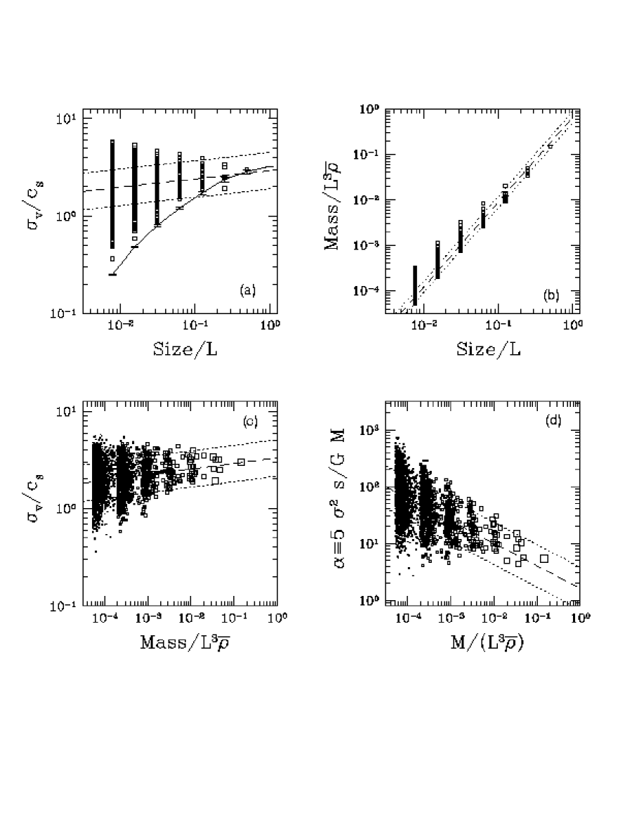
Figure 10: Scale dependence of kinetic quantities in a projected map. In (a)-(d), each point represents one of the square regions of contrast (ROCs) identified in Fig. (9), with edge size $s$. In (a), we plot vs. size $s$ (normalized to the box length $L$) the dispersion of the line-of-sight velocity $\sigma_{v}$ in each projected square ROC, and also show (solid line) the mean dispersion in line-of-sight velocity for 3D cubes of side $s$. In (b), we plot vs. $s/L$ the mass $M$ of each ROC (normalized to the total mass in the simulation box $\bar{\rho}L^{3}$. In (c), we show $\sigma_{v}$ vs. $M$. In (d), we show the virial parameter $\alpha$ vs. $M$. In each frame, dashed lines represent linear least-squares fits to the data; dotted lines represent 1-sigma deviations from the fit. In (c) and (d), we plot points from different-sized regions with different expansion factors.

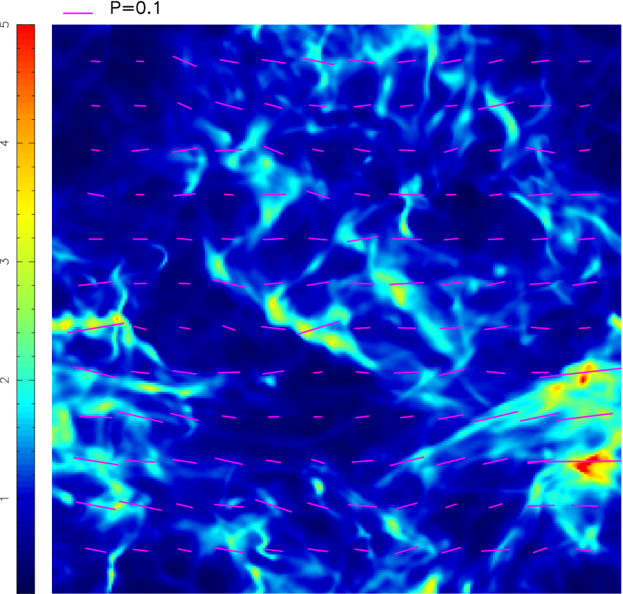
Figure 22: Column density (color scale, with units $\bar{\rho}L$) and simulated polarization map for model snapshot B2 ($\beta=0.01$, ${\cal M}=7$), projected along $\hat{z}$ perpendicular to the mean magnetic field. The fractional polarization at each point is proportional to the value of a fiducial polarization $P$ corresponding to a uniform medium and uniform magnetic field perpendicular to the line of sight, arbitrarily set here to $P=0.1$ as shown in the key.

Figure (9) shows an example of how the ROCs at multiple scales are distributed on the map of model snapshot B2 projected in the $\hat{z}$ direction (Figure 22 shows a colorscale image of the column density for the same snapshot projection). For the ROC ensemble shown in the figure, we compute masses, velocity dispersions, and values of the so-called virial parameter $\alpha\equiv 5\sigma_{v}^{2}s/GM$ Bertoldi & McKee (1992). In Figure (10), we plot the values as a function of (linear) size scale and/or mass. We also evaluate least-squares linear fits to $d\log(\sigma_{v})/d\log(s)$, $d\log(M)/d\log(s)$, $d\log(\sigma_{v})/d\log(M)$, and $d\log(\alpha)/d\log(s)$; the respective values in this example are $0.09$, $1.87$, $0.06$, and $-0.4$.

From parts (a) and (c) of Figure (10), it is clear that although the there is a mean increase in velocity dispersion with mass and linear size, there is a great deal of scatter as well. The upper envelopes of the velocity dispersion distributions in fact even decrease as a function of increasing $M$ and $s$; the lower envelopes increase more steeply. The distribution of $\alpha$ vs. $M$ also shows large dispersion, with a nearly-flat lower envelope and an upper envelope showing a decrease in $\alpha$ with $M$. The $M$ vs. $s$ distribution has a relatively low dispersion.

Many of the features evident in Figure (10) can be understood by reference to the scaling properties of the underlying three-dimensional distribution, together with the effects of projection onto a plane. First consider the $\log(\sigma_{v})$ - $\log(s)$ distribution. The procedure we have used to identify ROCs in the projected plane also can be used in the 3D data cube itself; we can then compute the mass and velocity dispersion for each 3D cell of edge size $s$ that meets the contrast criterion. In Figure (10 a), we show how the mean velocity dispersion for these 3D cells depends on size scale. Interestingly, this curve traces fairly closely the lower envelope of the distribution of $\sigma_{v}$ vs. projected size for ROCs on the projected plane. Thus, for nearly all projected regions of area $s\times s$, the majority the velocity dispersion can be attributed to the superposition along the line-of-sight of many regions of volume $s\times s\times s$ with different mean velocities. The relatively weak dependence of mean linewidth on projected size (or mass) simply reflects the ubiquity of “contamination” by foreground and background material. Previously, Issa, MacLaren, & Wolfendale (1990) and Adler & Roberts (1992) have made a related point that inferred broad linewidths of apparently quite massive GMCs may arise due to overlapping in velocity space of narrower velocity distributions from individual smaller clouds superimposed along the line of sight. Relatively steep increases of linewidth with size, as reported by Larson (1981) and subsequent authors, may be obtained in observations provided that a structure is distinguishable from its surrounding by a sufficient density or chemical contrast; these steeper laws correspond to what we measure with our 3D ROC procedure (solid lines in 10a, 11a).

In Fig. (10b), we show the distribution of mass with projected size for the ROCs; the mean logarithmic slope is nearly equal to two – rather than three, as would be the case for compact objects with three comparable dimensions. The mean slope is close to two simply because each ROC samples along the entire line-of-sight so that mass is nearly proportional to projected area; note, however, that at small scales, the masses can lie considerably above the mean fit.

It is interesting to compare the virial parameter $\alpha$ vs. $M$ distribution shown in Figure (10) with the analogous plot presented by Bertoldi & McKee (1992) analyzing the properties of apparent clumps in four different observed clouds. For the data sets considered in that work, linear fits to the $\log\alpha$ vs. $\log M$ relation gave slopes between $-0.5$ and $-0.68$. For the model data shown in Fig. (10) (and for our other snapshots as well), the mean fit has a somewhat shallower slope. But the upper envelope of this distribution (and those for other snapshots) has slope $\sim-0.5$ to $-0.6$. We can understand this upper envelope as follows: First, the largest velocity dispersions at a given projected scale (cf. Fig. 10a) are nearly independent of scale (typical logarithmic slope is $\sim 0$ to $-0.1$). With this, together with the mass scaling nearly as $s^{2}$, the result is an upper envelope of $\alpha\propto M^{-0.5}-M^{-0.6}$. The relatively flat lower envelope of the $\alpha$ vs. $M$ distribution can be explained by the projected ROCs that sample the $\sigma_{v}\propto s^{0.5}$ lower-envelope of the linewidth-size distribution (following the true 3D linewidth-size relation), together with the approximate $M\propto s^{2}$ scaling.

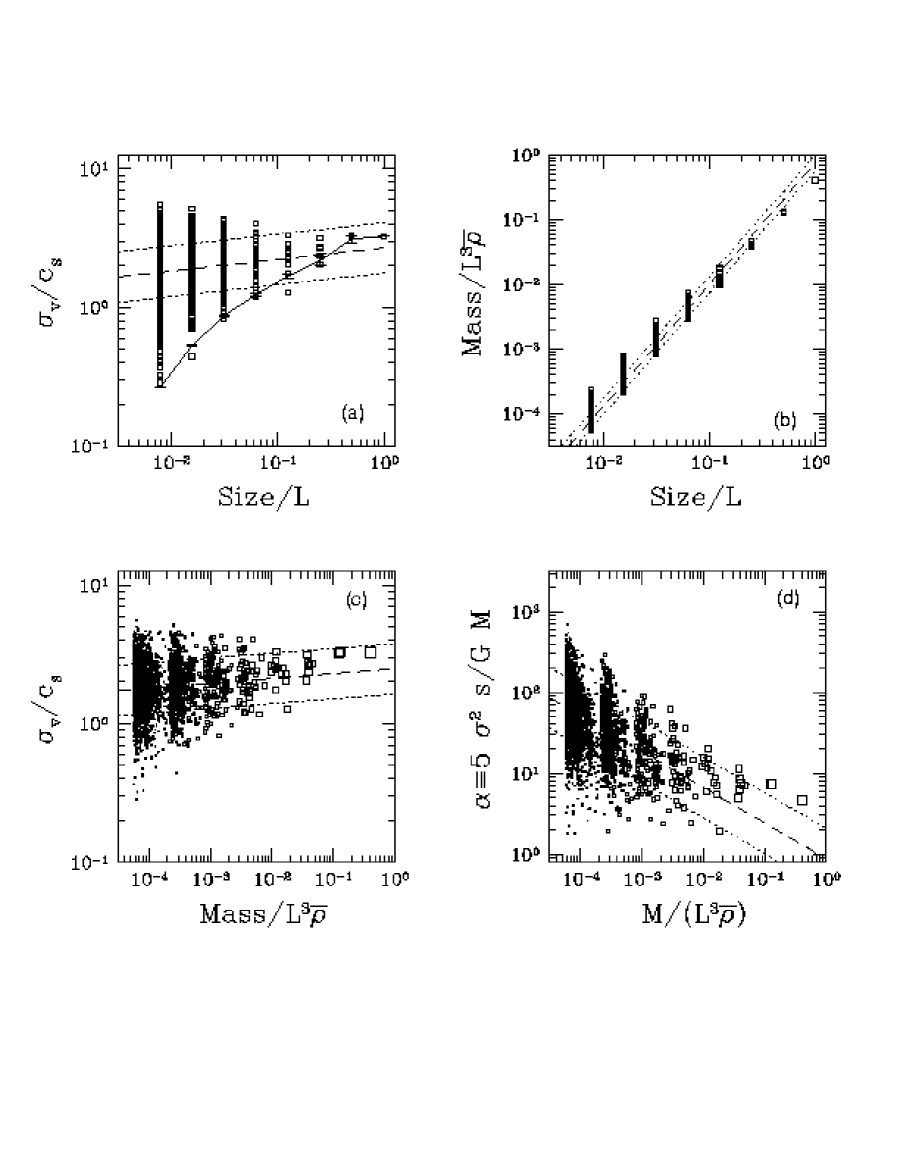
Figure 11: Same as in Fig. 10, for model snapshot D2.

All of the other model snapshots show qualitatively similar distributions of the kinetic parameters for ROCs to those shown in Figure (10). For example, we show the same distributions obtained for a weak-magnetic-field model snapshot (D2) in Figure (11); qualitatively, all of the kinetic scalings are quite comparable to those obtained for the strong-magnetic-field model. In general, for the model snapshots in Table 2, the projections parallel to the magnetic field axes yield slightly stronger increase of linewidth with size than do the other projections. For projections perpendicular to the mean field, the ranges in the fits for the different snapshots are $d\log(\sigma_{v})/d\log(s)=0.07-0.12$, $d\log(\sigma_{v})/d\log(M)=0.03-0.08$, and $d\log(\alpha)/d\log(s)=-0.45$ to $-0.34$ (using the same minimum surface density contrast factor $f_{c}=1$ and $\rho_{min}=3\bar{\rho}$). For projections parallel to the mean field, the respective ranges for these fits are $0.11-0.19$, $0.06-0.12$, and $-0.40$ to $-0.29$. The fits to $d\log(M)/d\log(s)$ have a very small range, $1.83-1.89$, for all projections (using $f_{c}=1$ and $\rho_{min}=3\bar{\rho}$).

The results depend weakly on the definition of a ROC, and in particular on $\rho_{min}$. Reducing $\rho_{min}$ tends to yield flatter slopes for $d\log(\sigma_{v})/d\log(s)$ and $d\log(\sigma_{v})/d\log(M)$ (because velocity is anticorrelated with density, so that additional low-density material along the line of sight increases the dispersion closer to the maximum), and steeper slopes for $d\log(M)/d\log(s)$ (approaching 2, the limiting form for uniform column density), and for $d\log(\alpha)/d\log(s)$ (approaching $-0.5$, the limiting form for velocity dispersion independent of size and uniform column density). Increasing $\rho_{min}$ has the opposite effect. The changes in slopes come about mainly from variations in the loci of the lower envelopes of the distributions when $\rho_{min}$ varies; the upper envelopes change very little, since they reflect the kinetic properties of ROCs which sample through the largest possible portion of the model cloud.

Because the projected ROC identification algorithm does not take into account any line-of-sight information for the material in any projected region, it should not be surprising that the velocity dispersions for projected regions can be much larger than the velocity dispersions for 3D cubes with the same projected size. One might argue that foreground and background material extraneous to a principal condensation could easily be removed based on velocity information, so that structures identified as contrasting regions in observed molecular line $l-b-v$ data cubes would truly represent spatially coherent structures. Examination of the line-of-sight velocity and line-of-sight position distributions for individual projected ROCs, however, suggests that it may in fact be difficult to eliminate foreground/background contamination.

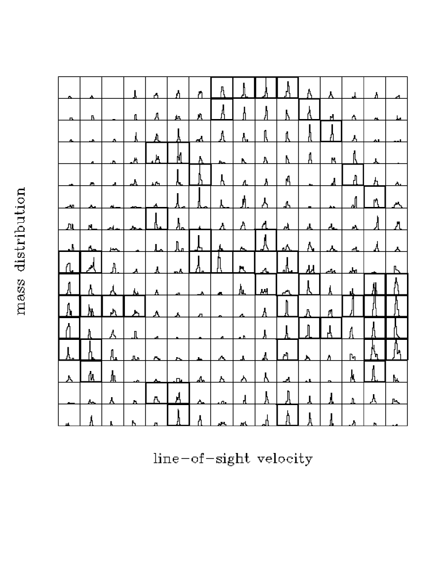
Figure 14: Same as Fig. (12), for projected region size $s=L/16$.

To illustrate the problem, Figure (12) shows histograms of line-of-sight velocity (equivalent to a line profile for an optically-thin tracer uniformly excited above $\rho_{min}=3\bar{\rho}$) for regions of projected linear scale $s=L/8$. Although some of the line shapes are irregular, none of those meeting the ROC criterion (in this example) are clearly multicomponent distributions. For comparison, in Figure (13), we show the distribution of mass with position along the line of sight. Evidently almost every region - both ROCs and non-ROCs – has multiple spatial components along the line-of-sight. Figures (14) and (15) show the same distributions for spatial regions at higher resolution; again, almost all velocity profiles are single component, while spatial distributions are multicomponent. By dividing our data cubes in half and computing velocity histograms separately for the “front” and “back” halves, we have checked that the ubiquity of single-component velocity distributions is not an artifact of periodic boundary conditions. We have also checked that the phenomenon of multi-spatial component/ single-velocity component ROCs is still prevalent even when the density threshold $\rho_{min}$ is set higher; for example, Figure 16 a,b shows the velocity and position distributions for the same model as before, but now with $\rho_{min}=10\bar{\rho}$. A complementary phenomenon that we have also identified in several model projections is that multiple velocity components in a given ROC may correspond to a single extended spatial component – as a consequence, for example of two “colliding” clumps being viewed during a merger along the line-of-sight.

The general lack of correspondence between structures in position and velocity space in ISM models has previously been noted, based on various sorts of analyses. For example, Adler & Roberts (1992) analyze the model galactic disks generated from two-dimensional N-body cloud-fluid simulations, and show that apparent single “clouds” in longitude-velocity space are often highly extended along the line-of-sight, and that what appears to be a single GMC in a spatial plot may be assigned to multiple “clouds” in longitude-velocity space. Pichardo et al (2000) show that the morphology of structures in position-position-velocity space (equivalent to channel maps) in their 3D MHD simulations is more strongly correlated with velocity structures in physical space than with density structures in physical space.

The current analyses and previous work on this question do not treat molecular excitation and radiative transfer in detail. Studies that do include these complex effects will be required to reach definitive conclusions on the relation between maps of molecular lines and 3D physical density-temperature-velocity cubes. If spatially compact regions have substantially higher molecular excitation than more diffuse surroundings due to line trapping, then it is still possible that velocity information could be used to separate spatially-connected clumps from foreground and background material. Large amplitude rotation of clouds, if present, would also help to differentiate superposed line-of-sight clumps in the velocity domain. Potentially, methods that use specific information about spectral line shapes (e.g. Roslowsky et al (1999)) may also be adapted to discriminate spatially-separated regions. The present simplified analysis suggests, however, that foreground and background material may at least significantly increase the dispersion in the linewidth-size distributions for clumps identified from molecular emission data cubes (e.g. Williams, de Geus, & Blitz (1994), Stutzki & Güsten (1990)).

6 Magnetic field distributions and simulated polarization

We now turn to magnetic field structure, and begin by considering how the distribution of the magnetic field varies for models with different mean magnetization. As seen in Figure 1d, the rms magnetic field strength initially increases, due to the generation of perturbed field by velocity shear and compression. The distribution of the individual components of $\bf B$ for matched Mach number model snapshots B2,C2,D2 is shown in Figure 17. The dimensionless field strength ${\cal B}\equiv B/(4\pi\bar{\rho}c_{s}^{2})^{1/2}$ that we report can be converted to a physical value using

$$B=1.4\times{\cal B}\times(T/10{\rm K})^{1/2}(n_{H_{2}}/10^{2}{\rm cm}^{-3})^{1/2}\ \mu{\rm G}.$$ (15)

As illustrated by the figure, the component distributions are more nearly Gaussian for the case of stronger magnetic fields; this is true for all of the model snapshots, although the distributions in the high-$\beta$ (low-$B_{0}$) cases do become more Gaussian in time. For the weak-field models, the dispersion in each component of the magnetic field is larger than the mean field component.

Because magnetic fields are measured via the Zeeman effect with different atomic and molecular tracers in different density regimes, it is interesting to analyze how the mean field strength in simulations may depend on density. Since the magnetic field is weaker and less able to resist being pushed around by the matter in the $\beta=0.1,1$ (C and D) simulations, one expects that the field strength will have stronger density dependence for these models than for the $\beta=0.01$ simulation. This is indeed the case, as can be seen in Figure 18. Particularly at densities below the mean, the magnetic field strengths in the high-$\beta$ models are strongly density dependent; the low-density slope of $d\log B/d\log\rho$ for these models is near the value $2/3$ associated with a constant ratio of mass to magnetic flux and isotropic volume changes.

At high densities (above $\sim 10\bar{\rho}$) the relatively flat slope of the $\beta=0.01$ model increases, becoming comparable to the slopes of the $\beta=0.1,1$ models. Figure 19 shows the high-density $B$ vs. $\rho$ dependence, for various model snapshots; fits for fiducial density $n_{H_{2}}$ in the range $10^{3}-10^{4}{\rm cm}^{-3}$ (i.e. $\rho/\bar{\rho}=10$ to $100$) yield slopes $0.3-0.7$ for $d\log B/d\log\rho$. Only the Mach-9 $\beta=1$ model yields a high-density-regime slope as steep as the isotropic contraction limit. The other snapshots have slopes 0.3-0.5, which may be compared with the slope 0.47 found from a compilation of Zeeman measurements at high densities $n_{H_{2}}=10^{2}-10^{7}{\rm cm}^{-3}$ (Crutcher, 1999). The values of the mean $B^{2}$ in any density regime generally increase with increasing mean net magnetic flux $B_{0}$ (i.e. decreasing $\beta$), but because there is significant dispersion about the mean $B^{2}$, there is considerable overlap of the $1-\sigma$ deviation regions among the different model snapshots (Fig. 18).

The numerical results on the $B$ vs. $\rho$ relation presented by Padoan & Nordlund (1999) (see their Fig. 7) are qualitatively similar to our results, with some differences apparent at the high density end. The lower Mach number in their low-$\beta$ model compared to their high-$\beta$ model likely accounts for its relatively weaker increase of $B$ with $\rho$ at high density, compared to our results. We also differ with those authors regarding the astronomical implications of the numerical results. In particular, we do not attempt a comparison of the low-density end of the $B$ vs. $\rho$ distributions with observations made in the diffuse ISM, because (a) the physical regime modeled by the simulations is not appropriate for the diffuse ISM (where thermal pressure is comparable to, rather than much smaller than, $\langle\rho v^{2}\rangle$); and (b) the transformation from simulation to physical variables for local magnetic field values involves multiplying by the mean magnetic field $B_{0}$ on the largest scale, and this need not be the same in the diffuse and cold ISM ($\beta$ parameterizes this mean field strength). We conclude that the $B$ vs. $\rho$ relations obtained from simulations do not at present constrain the value of $\beta$. At high densities, all models (either weak or strong $B_{0}$ on the large scale) yield slopes which are consistent with high-density molecular Zeeman observations. At very low densities, where the predictions of models with varying $\beta$ do differ, estimating $B$ within clouds would be difficult, since HI Zeeman observations probe the high columns of foreground and background material, rather than the low column of cloud material (although velocity information may help; cf. Goodman & Heiles (1994)). The field strengths in the low density regions within molecular clouds may in fact be systematically higher than those at comparable density in the diffuse ISM.

For all the snapshots, there is significant dispersion in the total magnetic field strength. In addition to this overall dispersion in magnitude, there is a dispersion in the magnetic field vector direction which increases with decreasing strength of the mean field component $B_{0}$, simply because fixed amplitude fluctuations have larger relative amplitudes compared to a weak mean magnetic field. The dispersion in field directions has important consequences for any observational measurement of the mean magnetic field via Zeeman splitting. Observations of Zeeman splitting at any position on a map yield the line-of-sight average value for the line-of-sight magnetic field, weighted at each point along the line-of-sight by the local excitation. When a given line of sight has many fluctuations in the direction of the magnetic field, the average value of $\langle B_{los}\rangle$ will be small, even if individual local components of the field have large magnitudes.

To demonstrate how the averaged line-of-sight field components vary with mean field strength and observer orientation, we depict in Figure 20 an overlay of $\langle B_{los}\rangle$ on the column density for three model snapshots with matched Mach number. In Figure 21, we plot the values of $\langle B_{los}\rangle$ vs. column density of dense gas. The Figures show, unsurprisingly, that the line-of-sight-averaged magnetic field strengths are greatest when the mean field $B_{0}$ is largest and is oriented along the observer’s line-of-sight (top left panel). For the weaker-field models, the average line-of-sight field is lower, and there is larger dispersion. For all the snapshots, there is considerable dispersion in the values of $\langle B_{los}\rangle$ on the map, and the largest values do not correspond to the positions of highest column density; in fact, there is some tendency of line-of-sight-averaged field to anticorrelate with column density. Thus, although the local field strength $|B|$ increases with density (cf. Figs 18, 19) and may be much larger than the volume-averaged mean field $B_{0}$ for the entire box, line-of-sight superpositions of non-aligned vector components produce average line-of-sight field strengths closer to the large-scale volume-averaged value.

It is well known that it is difficult to detect the Zeeman effect in molecular clouds (e.g. Heiles et al. (1993)) because the frequency splitting is small when the field is weak. This, coupled with the possibility (cf. Fig. 21) that an impractically large number of measurements might be required to obtain statististically-significant results for the large-scale field, underscores the importance of supplementing programs of direct detection with other methods for estimating the mean field strength. Long before direct Zeeman detections were first made, Chandrasekhar & Fermi (1953) estimated mean spiral-arm field strengths $B_{0}$ from the mean gas density, line-of-sight velocity dispersion, and the dispersion in orientations of the magnetic field in the plane of the sky. The field line orientation is taken to be traced by the polarization direction for background stars, which occurs provided that the dust grains producing the intervening extinction are aligned with short axes preferentially parallel to $\bf B$, and so preferentially extinguish linear polarizations perpendicular to $\bf B$.

The Chandrasekhar & Fermi (1953) (hereafter CF) estimate is based on the fact that for linear-amplitude transverse MHD (Alfvén) waves, $B_{p}=\sqrt{4\pi\bar{\rho}}|\delta{\bf v}|/(|\delta{\bf B}|/B_{p}).$ Here $B_{p}$ is the projection of the mean magnetic field on the plane of the sky, and $\delta{\bf B}$ and $\delta{\bf v}$ are the components of the magnetic and velocity perturbations in the plane of the sky transverse to ${\bf B}_{p}$. If the interstellar polarization is parallel to the local direction of ${\bf B}_{p}$, then the ratio $|\delta{\bf B}|/B_{p}$ in the denominator may be replaced by the dispersion $\delta\phi$ in polarization angles (for small angle/low amplitude perturbations). With the further assumption that the true velocity perturbations are isotropic, then the dispersion in the transverse velocity $|\delta{\bf v}|$ is equal to the rms line-of-sight velocity $\delta{v_{los}}$. We thus obtain

$$B_{p}={\cal Q}\sqrt{4\pi\bar{\rho}}\ \delta{v_{los}}\ \delta\phi^{-1}$$ (16)

where, for CF’s field model, ${\cal Q}=1$. Modifications to the CF formula allowing for inhomogeneity and line-of-sight averaging are discussed by Zweibel (1990) and Myers & Goodman (1991), respectively. Both of these effects (and others; see Zweibel (1996)) tend to reduce ${\cal Q}$.

Potentially, the CF “polarization-dispersion” method can be used to estimate plane-of-sky magnetic field strengths on scales within turbulent interstellar clouds. It may also be possible to combine these results with Zeeman measurements to estimate the total magnetic field strength (Myers & Goodman, 1991; Goodman & Heiles, 1994). In order to evaluate the ability of the CF method to measure mean plane-of sky field strengths, we provide a first (simplified) test of it using our model turbulent clouds. For this test, we have created simulated polarization maps for each cloud by integrating the Stokes parameters along the line-of-sight over a projected grid of positions, assuming the polarizability in each volume element is proportional to the local density. The details of this procedure, together with a more extensive discussion of simulated polarization distributions, will appear in a separate publication (Ostriker et al, 2000).

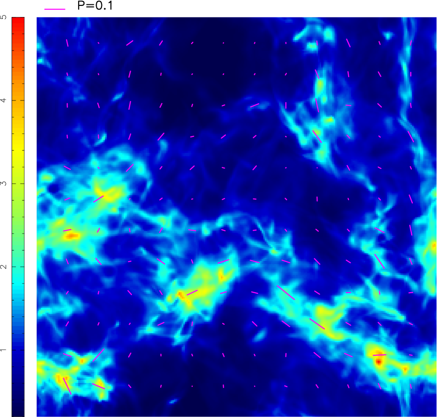
Figure 23: Column density and polarization map for model snapshot D2 ($\beta=1$, ${\cal M}=7$), projected along $\hat{z}$; definitions as in Fig. 22.

For two projected model snapshots (B2 with $\beta=0.01$ and D2 with $\beta=1$ projected along $\hat{z}$), Figures 22 and 23 show examples of the polarization maps overlaid on color scale column density maps. The analogous map (not shown) for the model C2 ($\beta=0.1$) looks quite similar to Figure 23. From the figures, it it immediately clear that the model with a stronger mean magnetic field $B_{0}$ has more ordered polarization directions and larger typical values of the fractional polarization, compared to the model with a weaker mean magnetic field. These trends are as expected: a weaker mean field has lower tensile strength, so that for a given level of kinetic energy the Reynolds stresses will produce larger fractional perturbations in the magnetic field – corresponding to larger fluctuations in projected line-of-sight averaged position angle. Also, because of the larger dispersion in local polarization directions along any line of sight, cases with weaker mean magnetic fields will show lower net polarization through the cloud (from the line-of-sight averaging of the varying local vector directions). While local (line-of-sight averaged) polarization directions may have any orientation with respect to local projected surface density, there is some tendency for the large-scale projected density and large-scale polarization directions to align in the high-$\beta$ (but not low $\beta$) models, because the magnetic field and density are both strongly sheared and compressed by the large-scale, large-amplitude velocity field.

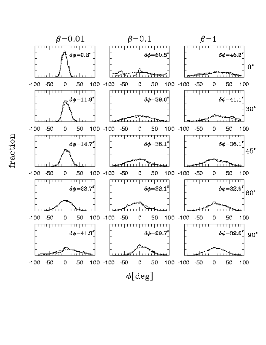
Figure 24: Distribution of polarization angles for projections of models with matched kinetic energy and differing mean magnetic field strength. Left, center, and right columns respectively show projections of strong, moderate, and weak-$B_{0}$ cases (from ${\cal M}=7$ snapshots B2, C2, D2), for the mean magnetic field direction lying at varying angles with respect to the plane of the sky (0, 30, 45, 60, and 90^∘, from top to bottom). Each panel shows a histogram of the distribution of polarization position angles with respect to the most-frequent direction, in degrees. Labels in each panel give the dispersion of the distribution. Dashed curves show Gaussian fits.

In Figure 24, we show the distributions of polarization angle at various “observer” orientations for models with matched kinetic energy and mean magnetic field strengths at three different levels ($\beta=0.01,0.1,1$, corresponding to fiducial $B=14,4.4,$ and $1.4\mu{\rm G}$ from eq. 15). As is clear from the Figure, only the strong-field model has significantly correlated directions in the simulated polarization vectors. This is expected, since only this model has perturbed magnetic energy lower than the mean magnetic energy; the ratios are $\delta B^{2}/B_{0}^{2}$ are 0.27, 4.0, and 12, respectively, for the snapshots presented.

For the cases shown in Figure 24 where the angle dispersion $\delta\phi$ is $25^{\circ}$ or less (i.e. the $\beta=0.01$ projections at $i=0,30,45,$ and $60^{\circ}$), we have compared the known value of the mean plane-of-sky magnetic field $B_{p}\equiv B_{0}\cos(i)$ with the Chandrasekhar-Fermi estimate. We find that $\cal Q$ (see equation (16)) is in the range 0.46-0.51. This suggests that the CF estimate, modified by a multiplicative factor $\sim 0.5$ to account for a more complex magnetic field and density structure, can indeed provide an accurate measurement of the plane-of-sky magnetic field when the polarization angle fluctuations are relatively small. The method fails, however, when the polarization angle fluctuations are large. We will present a more comprehensive analysis of this promising diagnostic in a separate publication.

7 Summary and discussion of structural analyses

With modern high-performance computational tools, it is possible to create and evolve simulated dynamical representations of turbulent, magnetized clouds at comparable plane-of-sky spatial resolution to that of radio-wavelength observational maps of GMCs. This paper reports on the properties of a set of such simulations.

We start by briefly summarizing (§3) the results on energy evolution in our simulations. We confirm the conclusions from our previous work that turbulent decay is rapid even in magnetized models, finding that an interval of only 0.4-0.8 flow crossing times is sufficient to reduce the total turbulent energy by a factor two from its initial value; the corresponding physical time for GMC parameters is only a 2-4 million years. We also confirm that in situations where turbulence is not replenished, the criterion for a cloud to collapse gravitationally depends only on whether it is sub- or super-critical with respect to its mean magnetic field; the characteristic collapse time in the latter case is $\sim 6$ Myr for GMC parameters.

Following the presentation of energetics, the bulk of the paper (§§4-6) is concerned with developing tools for structural analyses and applying them to our simulated data cubes. Although simplified in their treatment of small scales (ambipolar diffusion is neglected) and thermal properties (a constant gas temperature is assumed), the 3D data cube “snapshots” from our numerical experiments provide a detailed portrait of the density, velocity, and magnetic field structure in the simulated clouds. This structural portrait is dynamically self-consistent in that it is an instantaneous solution to the full time-dependent MHD equations: the density and magnetic field variables have evolved in response to a (time-dependent) turbulent velocity field, which itself has evolved subject to gas pressure gradient forces, magnetic stresses, and self-gravity.

Model cloud snapshots from simulations provide a unique opportunity to (i) explore the intrinsic character of 3D structure in magnetized gaseous systems subject to supersonic turbulence, and (ii) determine which aspects of the observed properties of GMCs (from 2D plane-of-sky integrated maps or $l-b-v$ data cubes) can be explained as a manifestation of their internal turbulence. The possibilities for such exploration are enormous; for practical purposes, we have limited the scope of this paper to three groups of analyses. We consider: (1) the distributions of mass, volume, and area as functions of volume density and column density (§4); (2) the distributions of velocity dispersion, mass, and virial parameter $\alpha$ as a function of the spatial scale for zones in projected maps and cells in 3D cubes (§5); (3) the distributions of magnetic field strength vs. local volume density, line-of-sight-averaged line-of-sight magnetic field vs. column density, and distribution of simulated polarization angles (§6). For each of these analyses, we compare sets of cloud snapshots in which the turbulent Mach number is matched, and the large scale mean magnetic field strength $B_{0}$ varies by a factor ten, also allowing for different “observer” viewing angles. The rms tubulent velocities for the model snapshots are $\sigma_{v}=1-2\ {\rm km\,s^{-1}}$, and the mean magnetic field strengths are $B_{0}=1.4-14\ \mu{\rm G}$, assuming fiducial GMC parameters for volume-averaged density $n_{H_{2}}=100\ {\rm cm}^{-3}$ and temperature $T=10{\rm K}$.

The main results of these structural analyses are as follows:

1. The distribution of volume densities follows an approximately log-normal form, with densities of typical mass elements $\langle\rho\rangle_{M}$ compressed by a factor $\sim 3-6$ times the volume-averaged density $\bar{\rho}\equiv M/L^{3}$ for our sets of snapshots with Mach number ${\cal M}=\sigma_{v}/c_{s}$ in the range $5-9$ (see Fig. 3 and Table 2). This typical density contrast is comparable to that inferred for the concentrations in GMCs ($\langle\rho/\bar{\rho}\rangle_{M}\sim 6-8$) from ¹³CO molecular-line studies (cf. Paper III; Bally et al (1987); Williams, Blitz, & Stark (1995)). The corresponding rms mass-weighted dispersion in $\rho/\bar{\rho}$ is $\sim 3-13$. Although the density contrast generally increases with the value of the fast-magnetosonic Mach number ${\cal M}_{F}\equiv\sigma_{v}/\langle c_{s}^{2}+v_{A}^{2}\rangle^{1/2}$ (see Fig. 4), there is no obvious one-to-one functional relation between ${\cal M}$, $\beta\equiv c_{s}^{2}/v_{A,0}^{2}$, and the density contrast. In particular, the result obtained by Nordlund & Padoan (1999) for purely hydrodynamic quasi-steady turbulence of the relation between the density contrast and the Mach number $\cal M$ does not carry over for (evolving) MHD turbulence. When ${\cal M}\sim 5-9$, the Nordlund & Padoan (1999) quasi-steady hydrodynamic-turbulence result would predict mass-weighted means and dispersions of $\rho/\bar{\rho}$ in the range $\sim 7-21$ and $\sim 18-95$, respectively, larger than the range we find for our MHD models. Further investigation would be required to determine whether, for quasi-steady MHD turbulence, it is possible to find a clean functional relation between the mean (and dispersion) of $\rho/\bar{\rho}$ and the dimensionless parameters $\cal M$ and $\beta$ that is independent of the particular instantaneous turbulent power spectrum. Since, however, we expect that cold-ISM turbulence is subject to significant transient effects, and in addition large “cosmic variance” may result from low-$k$ dominance of the power spectrum, a one-to-one relation of this kind would probably not be realized in GMCs in any case.

2. The distributions of column densities $N$ also follow an approximately log-normal form, with mean logarithmic contrasts $\langle\log(N/\bar{N})\rangle$ an order of magnitude smaller that the mean logarithmic density contrasts $\langle\log(\rho/\bar{\rho})\rangle$ (see Figs. 5 – 8 and Table 2). The mass-weighted mean column density is thus just 7-35% greater than the area-weighted column density $\bar{N}\equiv\bar{\rho}L=M/L^{2}$, and the mass-weighted (area-weighted) dispersion in $N$ is 0.3-0.8 (0.3-0.6) times $\bar{N}$, for models with the range of Mach numbers and magnetic field strengths we have analyzed. Large-scale spatial correlation of the density perturbations is indicated by the log-normal, rather than Gaussian, form of the column density distributions. These large-scale spatial density correlations are associated with large-scale correlations in the velocity and magnetic fields (which, for the present models, are input in the initial conditions).

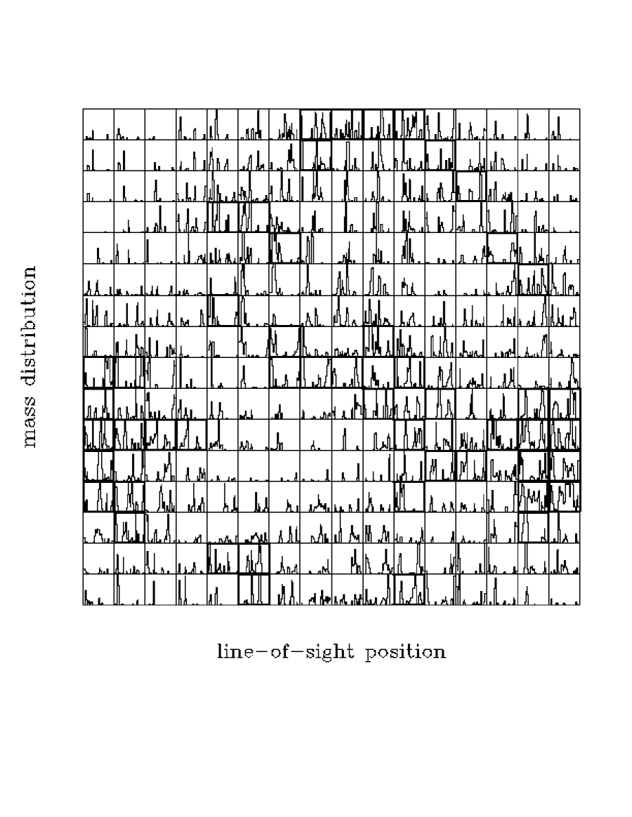
Figure 15: Same as Fig. (13), for projected region size $s=L/16$.

3. We use a binning algorithm to investigate the distribution of kinetic properties for plane-of-sky “clumps” as a function of the spatial clump scale. The clumps at a given scale are simply regions that contrast with the mean surface density at that scale; Fig. 9 shows an example of the maps of these so-defined regions of contrast (“ROCs”) at different scales. We find that there is a scatter in the values of line-of sight velocity dispersion averaged over projected regions of area $s^{2}$, ranging from the mean value of the velocity dispersion averaged over all cubes of size $s^{3}$ up to the velocity dispersion for the entire simulation of size $L^{3}$ (see Figs. 10, 11). The large velocity dispersions (“linewidths”) arise due to the superposition of many small volume elements with differing mean velocity along lines of sight through a given projected area. We show that ROCs which have single-component velocity distributions (“line profiles”) generally consist of several spatially separated components along the line-of-sight (see Figs. 12-16). Thus, what looks like a “clump” either on the plane of the sky or in position-velocity datacube may in fact be a superposition of spatially unconnected parts with smoothly overlapping velocity distributions.

4. We find that when mean magnetic fields $B_{0}$ are weak, there is a large scatter in the distribution of total magnetic field strength $|\bf B|$ in any given density regime, and that the mean value of $|\bf B|$ varies strongly with density (Fig. 18). For strong mean magnetic fields $B_{0}$ at moderate densities, there is less scatter in the distribution of $|\bf B|$, and a weaker variation of the mean value of $|\bf B|$ with density. At high densities, the variation of the mean of $|\bf B|$ with density is similar for all the models (Fig. 19), and is comparable to the indications of increasing field strength from Zeeman observations in high density tracers (Crutcher, 1999).

5. We show that, for the models considered here, the line-of-sight average of the line-of-sight magnetic field, $\langle B_{los}\rangle$, can vary widely across a projected map, and is not positively correlated with column density (see Figs. 20, 21). Because of the large scatter in $\langle B_{los}\rangle$, an accurate observational determination of the global average of $\langle B_{los}\rangle$ from the Zeeman method might require a very large number of pointings.

6. We have created simulated polarized-extinction maps by integrating the Stokes parameters along lines of sight for different simulation snapshots and orientations (Figs.22, 23). Because models with weak $B_{0}$ have much more variation in the vector direction of $\bf B$ at a given Mach number, the result is that they have lower average values of the polarization and larger dispersions in the polarization angle than their high-$B_{0}$ counterparts (Fig. 24). We show that the Chandrasekhar-Fermi formula can be slightly modified to estimate the plane-of-sky magnetic field strength $B_{p}$ in terms of the mean density $\bar{\rho}$, line-of-sight velocity dispersion $\delta v_{los}$, and plane of sky polarization angle $\delta\phi$ as $B_{p}\approx 1.8\bar{\rho}^{1/2}\delta v_{los}/\delta\phi$, provided $\delta\phi\lower 2.15277pt\hbox{$\;\buildrel<\over{\sim}\;$}25^{\circ}$.

One finding particularly notable for the interpretation of molecular-line observations concerns the nature of what have long been thought of as large-scale turbulent “clumps” within GMCs. The large scatter and relatively shallow mean slope for linewidth vs. projected size distributions of observed “clumps” (e.g. Williams, de Geus, & Blitz (1994); Stutzki & Güsten (1990)) is similar to that found for projected “regions of contrast” (ROCs) in our simulated clouds. The observed clumps are identified as coherent structures (peaks and their surroundings) in position-velocity molecular line data cubes; our ROCs are overdense on the plane of the sky and generally have single-component linewidths.

Because their linewidths are comparable to those of the larger cloud complexes in which they reside, the coherent structures in observed $l-b-v$ cubes have been interpreted as pressure-confined clumps (Bertoldi & McKee (1992)). We believe that these apparent pressure-confined clumps may in fact often be line-of-sight superpositions of spatially-unconnected condensations that collectively sample from the full turbulent velocity dispersion along the line-of-sight – hence appearing to have internal pressure comparable to that of the parent cloud as a whole. We find that the lower envelope of our linewidth-size distribution for ROCs closely follows the relation between mean linewidth and 3D cell size; it may be possible to apply a similar binning procedure to observational maps in order to deduce the true 3D mean linewidth-size relation.

Our structural analysis supports a revision (see references in §1 and §5 for related work) in the understanding of GMC clumps that parallels the recent paradigm shift in interpreting the cosmological Lyman-alpha forest. Namely, we suggest that the linewidths of these apparent clumps is due not to small-scale supersonic “microturbulence”, but to a superposition of bulk flows with a large range of correlation lengths. Unlike the situation in cosmology, however, we do not have a large-scale Hubble flow to spread out the velocity field and help us distinguish foreground and background concentrations. As a consequence, what appears to be a clump in projection may not, in three dimensions, be spatially compact or connected at all!

A further difference with the cosmological situation is that the overdense regions in clouds are not, in general, fated to collapse. The overdense regions are transient objects that form, and then disperse, from the effects of time-dependent velocity and magnetic fields. Eventually, through the overall dissipation of turbulence and the random superposition of temporary concentrations, a fraction of the material in a cloud must reach high enough densities to become strongly self-gravitating. The subsequent collapse and fragmentation, perhaps initiated at many independent sites in a cloud, must ultimately produce a collection of stars. The next generation of numerical simulations will require adaptive mesh algorithms to follow this gravitational collapse and fragmentation. Crucial questions are whether the spectrum of stellar masses that forms can ultimately be traced back to the bulk initial conditions (e.g. mean density, temperature, magnetic field strength, velocity dispersion) in the parent turbulent cloud, and what factors determine the overall rate of conversion of gas to stars.

Figure 1: Energy evolution of model clouds. Models with $\beta=0.01$, $0.1$, and $1$ are shown with dotted, solid, and dashed curves, respectively.

Figure 2: Evolution of turbulent energy $E_{turb}=E_{K}+\delta E_{B}$ in model clouds. Models with $\beta=0.01$, $0.1$, and $1$ are shown with dotted, solid, and dashed curves, respectively. The dot-dash lines indicate a slope $\propto t^{-1}$, for reference.

Figure 3: Comparative statistics of volume density in three model snapshots (B2, C2, D2 from Table 2) with matched Mach numbers ${\cal M}\sim 7$. Solid curves show fraction of volume as a function of density relative to the mean ($\rho/\bar{\rho}$); dashed curves show fraction of mass as a function of $\rho/\bar{\rho}$. Dotted curves show lognormal distributions with the same mean and dispersion as in each model snapshot.

Figure 4: Mass- and volume- weighted mean values of the logarithmic density contrast as a function of mean square fast magnetosonic Mach number from model snapshots in Table 2. Pentagons, squares, and triangles correspond to $\beta=0.01,0.1,$ and $1$, respectively. Dashed lines show $\left<\log(\rho/\bar{\rho})\right>_{M,V}=\pm 0.2(\log(1+{\cal M}_{F}^{2})+1)$

Figure 5: Comparative statistics of column density in three model snapshots (B2, C2, D2 from Table 2) with matched Mach numbers. Projection is along the $\hat{z}$ axis (perpendicular to the magnetic field). In each frame, left-displaced curves show fraction of projected area as a function of column density relative to the mean ($N/\bar{\rho}L\equiv N/\bar{N}$); right-displaced curves show fraction of mass as a function of $N/\bar{N}$. Dotted curves show lognormal distributions with the same mean and dispersion as in each model snapshot.

Figure 6: Comparative statistics of column density at full simulation resolution (a) and at resolution a factor four larger in linear scale (b); simulation data is from snapshot B2.

Figure 7: Same as in 5, except line-of-sight integration is only over $z>L/2$.

Figure 8: Comparison of (a) cumulative column density distribution for simulated cloud model (data from Fig. 7, with hexagons, squares, and triangles marking the $\beta=1,0.1,0.01$ model distributions) and (b) cumulative extinction distribution for the cloud IC5146. Dotted curves in both panels show cumulative log-normal fits.

Figure 9: Identification of regions of contrast (ROCs) as a function of spatial scale for data from model snapshot B2. Panels (a)-(g) outline regions that meet the contrast criterion at increasingly fine spatial resolution. A greyscale representation of the projected density is shown in (h) for comparison.

Figure 12: Distribution of mass with line-of-sight velocity for model snapshot B2 projected in the $\hat{z}$ direction, for regions of linear size $L/8$. Regions meeting surface density contrast criterion (cf. Fig. 9) are indicated with heavy outlines.

Figure 13: Distribution of mass with line-of-sight position for model snapshot B2 projected in the $\hat{z}$ direction, for regions of linear size $L/8$. Regions meeting surface density contrast criterion (cf. Fig. 9) are indicated with heavy outlines.

Figure 16: Same as Figs. (12), (13), for $\rho_{min}=10\bar{\rho}$.

Figure 17: Comparative statistics of magnetic field components for three model snapshots (B2, C2, D2 from Table 2) with matched Mach numbers. Solid, dotted, and dashed curves show fraction of mass as a function of $B_{x}$, $B_{y}$, and $B_{z}$, respectively. Mean field strengths are nonzero only in the $\hat{x}$ direction, with $B_{0}/(4\pi\bar{\rho}c_{s}^{2})^{1/2}=10,$ 3.16, and 1, for the top, middle, and bottom panels.

Figure 18: Dependence of the total magnetic field strength on density in three model snapshots (B2, C2, D2 from Table 2) with matched Mach numbers. Triangles, squares, and pentagons show the mean value of $B^{2}$ in each density bin for Mach-7 models with $\beta=0.01$, $0.1$, and 1, respectively. Shaded regions surrounding each curve corresponds to the $1-\sigma$ departures from the mean (errors in the means from counting statistics are smaller than the symbols shown). Dashed horizontal lines show the values of the square of the mean magnetic field, for the three models. Left and bottom scales give magnetic field strength $B^{2}$ and density $\rho$ in dimensionless units; right and top scales give corresponding fiducial values of $|B|$ and $n_{H_{2}}$ assuming $T=10$K and $\bar{n}_{H_{2}}=100{\rm cm}^{-3}$ for the temperature and volume-averaged density.

Figure 19: Density vs. mean total magnetic field strength at high densities for Mach-9 (top row) and Mach-7 (bottom row) model snapshots (fiducial values assume $T=10$K and $\bar{n}_{H_{2}}=100{\rm cm}^{-3}$). Error bars show expected (Poisson noise) error in determination of the means. Also shown (solid lines) are fits to $\log(B)$ vs. $\log(n)$ for $n_{H_{2}}>10^{3}{\rm cm}^{-3}$; the corresponding slope is indicated in each panel.

Figure 20: Mean line-of-sight-averaged magnetic field strength for Mach-7 model snapshots (B2 – left column, C2 – center column, D2 – right column) viewed from three orientations: along the mean field ($\hat{x}$; top row), at $45^{\circ}$ relative to the mean field (center row), perpendicular to the mean field ($\hat{z}$, bottom row). Contributions to $<B_{los}>$ are weighted by density, and include only zones with $\rho/\bar{\rho}>10$. Point size is scaled linearly by the value of $|<B_{los}>|$, with positive and negative values as shown by the key. For fiducial dimensional $B$ values, we adopt $T=10$K and $\bar{n}_{H_{2}}=100{\rm cm}^{-3}$. Only every 15th point in each direction on the grid is plotted, for clarity. Greyscale underlay shows the total column density for each projection.

Figure 21: Mean line-of-sight-averaged magnetic field strength $\langle B_{los}\rangle$ vs. column density $N$ of gas at $\rho/\bar{\rho}>10$ for model projections shown in Fig. 20. All points at $N/\bar{\rho}L>0.5$ are plotted; straight solid lines show linear least-squares fits. Dashed horizontal lines show the value of the volume-averaged mean line-of-sight field $B_{0}\sin i$ for each projection ($i$ is the angle between the plane of sky and $\bf B_{0}$).

References

- Adler & Roberts (1992) Adler, D.S., & Roberts, W.W. 1992, ApJ, 384, 95
- Alves et al (1998) Alves, J., Lada, C.J., Lada, E.A., Kenyon, S.J., & Phelps, R. 1998,ApJ, 506,292
- Ballesteros-Paredes, Vázquez-Semadeni, & Scalo (1999) Ballesteros-Paredes, J., Vázquez-Semadeni, E., & Scalo, J. 1999, ApJ, 515, 286
- Ballesteros-Paredes, Hartmann, & Vázquez-Semadeni (1999) Ballesteros-Paredes, J., Hatmann, L., & Vázquez-Semadeni, E. 1999, ApJ, 527, 285
- Bally et al (1987) Bally, J., Langer, W. D., Stark, A. A., & Wilson, R. W. 1987, ApJ, 312, L45
- Balsara et al (1999) Balsara, D. S., Pouquet, A., Ward-Thompson, D., & Crutcher, R.M. 1999, in Interstellar Turbulence, Proceedings of the 2nd Guillermo Haro Conference. Eds. J. Franco and A. Carraminana (Cambridge University Press), p.261 , p. 89
- Bertoldi & McKee (1992) Bertoldi, F., & McKee, C.F. 1992, ApJ, 395, 140
- Blitz (1993) Blitz, L. 1993, in Protostars and Planets III, ed. E. Levy & J. Lunine (Tucson: University of Arizona Press), p. 125
- Blitz & Williams (1997) Blitz, L., & Williams, J.P. 1997, ApJ, 488, L145
- Chandrasekhar & Fermi (1953) Chandrasekhar, S. & Fermi, E. 1953, ApJ, 118, 113
- Crutcher (1999) Crutcher, R.M. 1999, ApJ, 520, 706
- Elmegreen (1997) Elmegreen, B.G. 1997, ApJ, 480, 674
- Elmegreen (1999) Elmegreen, B.G. 1999, ApJ, 527, 266
- Elmegreen (2000) Elmegreen, B.G. 2000, ApJ, 530, 277
- Evans (1999) Evans, N.J. 1999, ARAA, 37, 311
- Evans & Hawley (1988) Evans, C. R., & Hawley, J. F. 1988, ApJ, 332, 659
- Gammie & Ostriker (1996) Gammie, C. F. & Ostriker, E. C. 1996, ApJ, 466, 814 (Paper I)
- Gammie, Stone, & Ostriker (2000) Gammie, C. F., Stone, J.M, & Ostriker, E. C., in preparation
- Goodman & Heiles (1994) Goodman, A.A., & Heiles, C. 1994, ApJ, 424, 208
- Hawley & Stone (1995) Hawley, J.F., & Stone, J.M. 1995, Computer Physics Communications 89, 127
- Heiles et al. (1993) Heiles, C., Goodman, A. A., McKee, C. F., & Zweibel, E. G. 1993, in Protostars and Planets III, ed. E. Levy & J. Lunine (Tucson: University of Arizona Press), p. 279
- Heyer & Schloerb (1997) Heyer, M., & Schloerb, P. 1997, ApJ475, 173
- Issa, MacLaren, & Wolfendale (1990) Issa, M., MacLaren, I., & Wolfendale, A.W. 1990, ApJ352, 132
- Klessen (2000) Klessen, R.S. 2000, ApJ, in press
- Klessen, Heitsch, & Mac Low (2000) Klessen, R.S. Heitsch, F., & Mac Low, M. (2000), ApJ, in press
- Lada et al (1994) Lada, C. J., Lada, E. A., Clemens, D. P., & Bally, J. 1994, ApJ, 429, 694
- Lada, Alves, & Lada (1999) Lada, C. J., Alves, J., & Lada, E. A. 1999, ApJ, 512, 250
- Larson (1981) Larson, R. B. 1981, MNRAS, 194, 809
- Mac Low et al (1998) Mac Low, M. M., Klessen, R. S., Burkert, A., & Smith, M. D. O. 1998, Phys.Rev.Lett. 80, 2754
- Mac Low (1999) Mac Low, M. M. 1999, ApJ, 524, 169
- Mac Low & Ossenkopf (2000) Mac Low, M. M., & Ossenkopf, V. 2000, A&A 353, 339
- Mestel & Spitzer (1956) Mestel, L., & Spitzer, L., Jr. 1956, MNRAS, 116, 503
- McKee (1999) McKee, C.F. 1999, in The Physics of Star Formation and Early Stellar Evolution, Eds. C. Lada, & N.Kylafis.
- McKee et al. (1993) McKee, C. F., Zweibel, E. G., Goodman, A. A., & Heiles, C. 1993, in Protostars and Planets III, ed. E. Levy & J. Lunine (Tucson: University of Arizona Press), p. 327
- McKee & Zweibel (1992) McKee, C.F., & Zweibel, E. G. 1992, ApJ, 399, 551
- Myers & Goodman (1991) Myers, P.C., & Goodman, A.A. 1991, ApJ, 373, 509
- Myers & Goodman (1988) Myers, P.C., & Goodman, A.A. 1988, ApJ, 329, 392
- Nordlund & Padoan (1999) Nordlund, Å., & Padoan, P. 1999, in Interstellar Turbulence, eds. J. Franco & A. Carramiñana, (Cambridge:CUP), p 218
- Ostriker, Gammie, & Stone (1999) Ostriker, E.C., Gammie, C.F., & Stone, J.M. 1999, ApJ, 513,259 (Paper III)
- Ostriker et al (2000) Ostriker, E.C. 2000, in preparation
- Padoan, Jones, & Nordlund (1997) Padoan, P., Jones, B. T., & Nordlund, Å. P. 1997, ApJ, 474, 730
- Padoan & Nordlund (1999) Padoan, P., & Nordlund, Å. 1999,ApJ, 526, 279
- Passot & Vázquez-Semadeni (1998) Passot, T. & Vázquez-Semadeni, E. 1998, Phys. Rev. E, 58, 4501
- Passot, Vázquez-Semadeni, & Pouquet (1995) Passot, T., Vázquez-Semadeni, E., & Pouquet, A. 1995, ApJ, 455, 536
- Pichardo et al (2000) Pichardo, B., Vázquez-Semadeni, E., Gazol, A., Passot, T., & Ballesteros-Paredes, J. 2000, ApJ, 532, 353
- Roslowsky et al (1999) Rosolowsky, E.W., Goodman, A.A., Wilner, D.J., & Williams, J.P. 1999, ApJ524, 887
- Scalo et al (1998) Scalo, J, Vázquez-Semadeni, E., Chappell, D., & Passot, T., 1998, ApJ504, 835
- Shu et al. (1987) Shu, F.H., Adams, F.C. & Lizano, S. 1987, ARA&A, 25, 23
- Shu et al (1999) Shu, F.H., Allen, A., Shang, H., Ostriker, E., & Li, Z.-Y. 1999, in The Physics of Star Formation and Early Stellar Evolution, Eds. C. Lada, & N.Kylafis.
- Solomon et al (1987) Solomon, P. M., Rivolo, A. R., Barrett, J., & Yahil, A. 1987, ApJ, 319, 730
- Stone & Norman (1992a) Stone, J. M. & Norman, M. L. 1992a, ApJSupp, 80, 753
- Stone & Norman (1992b) Stone, J. M. & Norman, M. L. 1992b, ApJSupp, 80, 791
- Stone, Ostriker, & Gammie (1998) Stone, J.M., Ostriker, E.C., & Gammie, C.F. 1998, ApJ, 508, L99 (Paper II)
- Stone, Gammie, & Ostriker (2000) Stone, J.M., Gammie, C.F., & Ostriker, E.C. 2000, in preparation
- Stutzki & Güsten (1990) Stutzki, J., & Gusten, R. 1990, ApJ, 356, 513
- Vázquez-Semadeni (1994) Vázquez-Semadeni, E., 1994, ApJ423, 681
- Vázquez-Semadeni, Ballesteros-Paredes, & Rodriguez (1997) Vázquez-Semadeni, E., Ballesteros-Paredes, J., & Rodriguez, L.F. 1997, ApJ474, 292
- Vázquez-Semadeni et al (2000) Vázquez-Semadeni, E., Ostriker, E., Passot, T., Gammie, C., & Stone, J. 2000, in Protostars and Planets IV, eds. Mannings, Boss, & Russell, (Tuscon:U.Arizona press) in press
- Williams, Blitz, & McKee (2000) Williams, J.P., Blitz, L., & McKee, C.F. 2000, in Protostars and Planets IV, eds. Mannings, Boss, & Russell, (Tuscon:U.Arizona press) in press
- Williams, Blitz, & Stark (1995) Williams, J. P., Blitz, L. & Stark, A. A. 1995, ApJ, 451, 252
- Williams, de Geus, & Blitz (1994) Williams, J.P., de Geus, E.J., & Blitz, L. 1994, ApJ, 428, 693
- Zuckerman & Palmer (1974) Zuckerman, B., & Palmer, P. 1974, ARAA, 12, 179
- Zweibel (1990) Zweibel, E.G. 1990, ApJ, 362, 545
- Zweibel (1996) Zweibel, E.G. 1996, in Polarimetry of the Interstellar Medium, eds. W.G. Roberge & D.C.B. Whittet, p. 486