Looking for a varying $\alpha$ in the Cosmic Microwave Background

Abstract

We perform a likelihood analysis of the recently released BOOMERanG and MAXIMA data, allowing for the possibility of a time-varying fine-structure constant. We find that in general this data prefers a value of $\alpha$ that was smaller in the past (which is in agreement with measurements of $\alpha$ from quasar observations). However, there are some interesting degeneracies in the problem which imply that strong statements about $\alpha$ can not be made using this method until independent accurate determinations of $\Omega_{b}h^{2}$ and $H_{0}$ are available.

We also show that a preferred lower value of $\alpha$ comes mainly from the data points around the first Doppler peak, whereas the main effect of the high-$\ell$ data points is to increase the preferred value for $\Omega_{b}h^{2}$ (while also tightening the constraints on $\Omega_{0}$ and $H_{0}$). We comment on some implications of our results.

I Introduction

There has been a recent growth of interest in theories where some of the usual constants of nature are actually time- and/or space-varying quantities. Most notably, the possibility of a time-varying fine-structure $\alpha$, has been the subject of a considerable amount of work, both at the theoretical and experimental/observational level.

From the theoretical point of view, the motivation comes from the recent work on the higher-dimensional theories [1], which are thought to be required to provide a consistent unification of the know fundamental interactions. In such theories the ‘effective’ three-dimensional constants are typically related to the ‘true’ higher-dimensional constants via the radii of the (compact) extra dimensions [2]. On the other hand, these radii often have a non-trivial evolution, naturally leading to the expectation of time (or even space) variations of the ‘effective’ coupling constants we can measure [3, 4, 5].

There are a number of different ways in which a variation of $\alpha$ can be modelled. From a ‘theoretical’ point of view, the more convenient one appears to be to interpret it as a variation in the speed of light $c$ [6, 7, 8, 9], but other alternatives have been explored [10]. It is also possible to analyse the consequences of the variation of $\alpha$ in a more phenomenological context, as was done in [11, 12].

On the observational level, the situation is at present somewhat confusing—see [13] for a brief summary. The best limit from laboratory experiments (using atomic clocks) is [14]

$$|{\dot{\alpha}}/\alpha|<3.7\times 10^{-14}yr^{-1}\,.$$ (1)

Measurements of isotope ratios in the Oklo natural reactor provide the strongest geophysical constraints [15],

$$|{\dot{\alpha}}/\alpha|<0.7\times 10^{-16}yr^{-1}\,,$$ (2)

although there are suggestions [16] that due to a number of nuclear physics uncertainties and model dependencies a more realistic bound is $|{\dot{\alpha}}/\alpha|<5\times 10^{-15}yr^{-1}$. Note that these measurements effectively probe timescales corresponding to a cosmological redshift of about $z\sim 0.1$ (compare with astrophysical measurements below).

Three kinds of astrophysical tests have been used. Firstly, big bang nucleosynthesis [17] can in principle provide rather strong constraints at very high redshifts, but it has a strong drawback in that one is always forced to make an assumption on how the neutron to proton mass difference depends on $\alpha$. This is needed to estimate the effect of a varying $\alpha$ on the ${}^{4}He$ abundance. The abundances of the other light elements depend much less strongly on this assumption, but on the other hand these abundances are much less well known observationally. Hence one can only find the relatively weak bound

$$|{\Delta\alpha}/\alpha|<2\times 10^{-2}\,,\qquad z\sim 10^{9}-10^{10}.$$ (3)

Secondly, observations of the fine splitting of quasar doublet absorption lines probe smaller redshifts, but should be much more reliable. Unfortunately, the two groups which have been actively studying this topic report different results. Webb and collaborators [18] were the first to report a positive result,

$$\Delta\alpha/\alpha=(-1.9\pm 0.5)\times 10^{-5}\,,\qquad z\sim 1.0-1.6$$ (4)

Note that this means that $\alpha$ was smaller in the past. Recently the same group reports two more (as yet unpublished) positive results [19], $\Delta\alpha/\alpha=(-0.75\pm 0.23)\times 10^{-5}$ for redshifts $z\sim 0.6-1.6$ and $\Delta\alpha/\alpha=(-0.74\pm 0.28)\times 10^{-5}$ for redshifts $z\sim 1.6-2.6$. On the other hand, Varshalovich and collaborators [13] report only a null result,

$$\Delta\alpha/\alpha=(-4.6\pm 4.3\pm 1.4)\times 10^{-5}\,,\qquad z\sim 2-4\,;$$ (5)

the first error bar corresponds to the statistical error while the second is the systematic one. This corresponds to the bound

$$|{\dot{\alpha}}/\alpha|<1.4\times 10^{-14}yr^{-1}$$ (6)

over a timescale of about $10^{10}$ years. It should be emphasised that the observational techniques used by both groups have significant differences, and it is presently not clear how the two compare when it comes to eliminating possible sources of systematic error.

Finally, a third option is the cosmic microwave background (CMB) [11]. This probes intermediate redshifts, but has the significant advantage that one has (or will soon have) highly accurate data.

The reason why the Cosmic Microwave Background is a good probe of variations of the fine-structure constant is that these alter the ionisation history of the universe [11, 12]. The dominant effect is a change in the redshift of recombination, due to a shift in the energy levels (and, in particular, the binding energy) of Hydrogen. The Thomson scattering cross-section is also changed for all particles, being proportional to $\alpha^{2}$. A smaller effect (which has so far been neglected) is expected to come from a change in the Helium abundance.

As is well known, CMB fluctuations are typically described in terms of spherical harmonics,

$$T(\theta,\phi)=\sum_{\ell m}a_{\ell m}Y_{\ell m}(\theta,\phi)\,,$$ (7)

from whose coefficients one defines

$$C_{\ell}=<|a_{\ell m}|^{2}>\,.$$ (8)

Increasing $\alpha$ increases the redshift of last-scattering, which corresponds to a smaller sound horizon. Since the position of the first Doppler peak (which we shall denote as $\ell_{peak}$) is inversely proportional to the sound horizon at last scattering, we see that increasing $\alpha$ will produce a larger $\ell_{peak}$ [12]. This larger redshift of last scattering also has the additional effect of producing a larger early ISW effect, and hence a larger amplitude of the first Doppler peak [11]. Finally, an increase in $\alpha$ decreases the high-$\ell$ diffusion damping (which is essentially due to the finite thickness of the last-scattering surface), and thus increases the power on very small scales.

The authors of [11] provide an analysis of these effects and conclude that future CMB experiments should be able to provide constraints on a varying $\alpha$ at the recombination epoch (that is, at redshifts $z\sim 1000$) at the level of

$$|{\dot{\alpha}}/\alpha|<7\times 10^{-13}yr^{-1}\,,$$ (9)

or equivalently

$$|\alpha^{-1}d\alpha/dz|<9\times 10^{-5}\,,$$ (10)

which seems to indicate that these constraints can only become competitive in the near future.

Here we analyse these effects for the BOOMERanG [20, 21] and MAXIMA [22, 23] data. We briefly review the method and then discuss the results in the next section. We find that this data tends to prefer a value of $\alpha$ that was lower in the past. However, we strongly emphasise that there are interesting and so far unnoticed degeneracies in the physics of the problem which imply that this method of determining the fine-structure constant can only produce strong constraints if other cosmological parameters are independently known. We will comment on this point in section III.

While this paper was being finalised, another preprint appeared [24], containing an independent analysis of the same data. It should be noticed that there are some significant differences in the two analysis procedures, as well as in the results, which we will point out along the way. In the cases where a direct comparison is possible, our work confirms their results, while in the other cases we provide some physical motivation for the differences.

II Data analysis

We perform a likelihood analysis of the recently released BOOMERanG [20] and MAXIMA [22] data, allowing for the possibility of a time-varying fine-structure constant. The method used follows the procedure described in [25, 26]. The angular power spectrum $C_{l}$ was obtained using a modified CMBFAST algorithm which allows a varying $\alpha$ parameter. We have changed the subroutine RECFAST [27] according to the extensive description given in [11].

We vary the power spectrum normalisation $C_{2}$ within the $95\%$ limits for the COBE 4-year data [28] The space of model parameters spans

$$\Omega_{0}=(0.1-1.0)\,,$$ (11)

$$\Omega_{b}h^{2}=(0.01-0.028)\,,$$ (12)

$$H_{0}=(50-80)\,,$$ (13)

$$\alpha/\alpha_{0}=(0.9-1.1)\,,$$ (14)

and the $C_{l}$ normalisation

$$bias=C_{2}/C_{2,COBE}=(0.83-1.16)\,.$$ (15)

Note that $\alpha_{0}$ is the value of the fine structure constant today. The basic grid of models was obtained considering parameter step sizes of 0.1 for $\Omega_{0}$; 0.003 for $\Omega_{b}h^{2}$; 5 for $H_{0}$; 0.01 for $\alpha/\alpha_{0}$ and finally 0.01 for the $bias$. In order to compute the maxima and the confidence intervals for the 1-dim marginalised distributions we have increased the grid resolution of each of the model parameters using interpolation procedures.

All our models have $\Omega_{total}=1$ and no tilt. We point out that this is in agreement [29] with the best-fit model for the $\Omega_{total}=1$ case for the combined analysis of the BOOMERanG and MAXIMA data. Somewhat surprisingly, the authors of [24] seem to find that the same data prefer tilted models even in the ‘standard’ case, that is without considering a varying fine-structure constant. This will obviously affect their results, as we will discuss below.

We also emphasise that $\alpha$ may or may not have had a different value at the nucleosynthesis epoch, which in particular will affect the value of $\Omega_{b}h^{2}$. Since in the present paper we do not treat this effect, the correct approach [8] is to accept the observationally determined value. This is the reason why we ignore excessively high values of $\Omega_{b}h^{2}$ which seem to be required by some analyses of the CMB data [21, 29].

For each of these $C_{l}$ spectra we compute the flat band power estimates of the CMB anisotropies obtaining a simulated observation for each data point. These estimates cover the multi-pole range sampled by both BOOMERanG and MAXIMA experiments. The values of $\Omega_{b}$ are obtained as function of $H_{0}$ in order to satisfy the range for $\Omega_{b}h^{2}$ defined above.

A The full dataset

Interesting conclusions can be drawn by comparing the nominal calibration case for both experiments with the Likelihood obtained after marginalising over the calibration uncertainties of BOOMERanG ($20\%$) and MAXIMA ($8\%$). As mentioned in [30] the fitting to a lower second Doppler peak can be achieved either by increasing the value of $\Omega_{b}h^{2}$ or decreasing the value of $\alpha/\alpha_{0}$. Note also that there is an additional constraint on $\alpha/\alpha_{0}$ coming from the position of the main acoustic peak [12]. We shall comment on the relative importance of the two constraints below.

For the nominal calibration case we obtain a best fit model with

$$H_{0}=55,\quad\Omega_{b}h^{2}=0.025,\quad\Omega_{0}=0.5\,,$$ (16)

$$\alpha/\alpha_{0}=0.94,\quad bias=0.87,\quad\chi^{2}=20.38\,.$$ (17)

In Fig 1 we plot the marginalised distributions for all the parameters.

For this case the maxima and confidence intervals for the marginalised distributions are as follows (all $1\sigma$): $\alpha/\alpha_{0}=0.96^{+0.02}_{-0.03}$, $H_{0}=50^{+16.02}_{-0.00}$, $\Omega_{b}h^{2}=0.026^{+0.002}_{-0.001}$, $\Omega_{0}=0.3^{+0.3}_{-0.1}$; $bias=0.9\pm 0.04$.

FIG. 1.: Marginal distributions for each model parameter for the nominal calibration case.

We then marginalised the 5-dim Likelihood function over the calibration uncertainties assuming a Gaussian prior. In this case we obtain a best fit model with

$$H_{0}=55,\quad\Omega_{b}h^{2}=0.025,\quad\Omega_{0}=0.4\,;$$ (18)

$$\alpha/\alpha_{0}=0.93,\quad bias=0.91,\quad\chi^{2}=15.55\,.$$ (19)

In Fig 2 we plot the marginalised distributions for all the parameters for the distribution marginalised over the calibration errors. Comparing with Fig 1 we notice that in the case of the marginalised distribution the distributions for $\Omega_{0}$ and $\alpha/\alpha_{0}$ are slightly shifted towards lower values, while those of $\Omega_{b}h^{2}$ and $H_{0}$ are not significantly affected.

The maxima and confidence intervals for the marginalised distributions are as follows (again, all are $1\sigma$): $\alpha/\alpha_{0}=0.94^{+0.03}_{-0.02}$, $H_{0}=50^{+16.62}_{-0.0}$; $\Omega_{b}h^{2}=0.026\pm 0.002$, $\Omega_{0}=0.3^{+0.17}_{-0.14}$, $bias=0.94\pm 0.07$.

FIG. 2.: Marginal distributions for each model parameter for the calibration marginalised distribution.

If we consider the best calibration case assuming a uniform prior we get the same best fit set of parameter values as for the calibration marginalised likelihood, apart from the bias (which now has the value $bias=0.84$). The best calibration factor is 1.0 (nominal) for BOOMERanG and 0.92 (ratio with respect to the nominal case) for MAXIMA (this corresponds to $\chi^{2}=15.73$). This is just telling us that if we keep BOOMERanG at the nominal calibration case and lower the height of the MAXIMA data points we force the normalisation of the models to decrease.

If instead we consider the best calibration case assuming a Gaussian prior we get a best fit with a calibration factor of 1.1 for BOOMERanG and 1.0 (nominal) for MAXIMA ($\chi^{2}=15.75$ before weighting). As should be expected we get a higher best fit value for the models normalisation of $bias=0.92$. Meanwhile for both cases we observe a decrease on the value of $\Omega_{0}$ from 0.5 to 0.4 and on the value of $\alpha/\alpha_{0}$ from 0.94 to 0.93, when compared with the nominal case.

Note that both pushing the BOOMERanG data up or pushing the MAXIMA data down provide for a better overlap of the two data sets. Then the different overall normalisations (in particular the height of the first Doppler peak) account for the different values of the cosmological parameters.

In fig 3 we plot the 2-dim Likelihood functions obtained after marginalising over the remaining three parameters. In Fig 4 we plot the likelihood surface for $H_{0}$ and $\alpha/\alpha_{0}$ as well as for $\Omega_{b}h^{2}$ and $H_{0}$. Similarly, Fig 5 contains the corresponding likelihoods for the nominal calibration case. This highlights the fact that there are some non-trivial degeneracies in the problem [31]. We shall return to this point below.

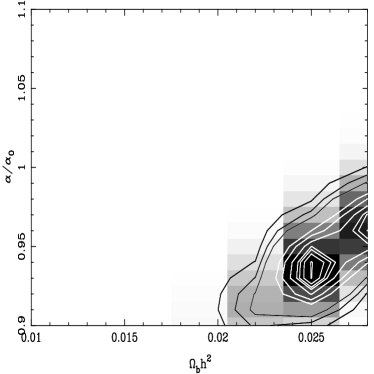
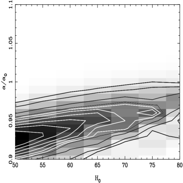
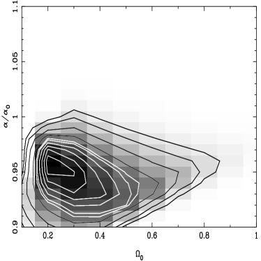
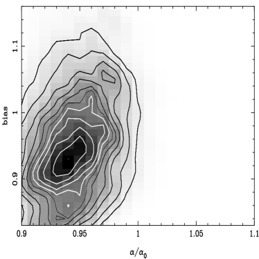
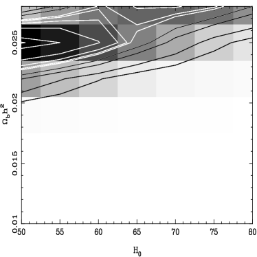
FIG. 3.: Confidence contours for the 2-dim distribution obtained after marginalising over the remaining three parameters (for the calibration marginalised distribution). Contours are at 10,20,30,…90 and 95 per cent confidence levels.

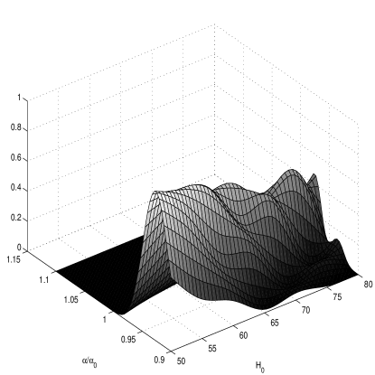
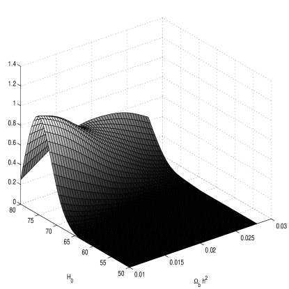
FIG. 4.: The likelihood surface for $H_{0}$ and $\alpha/\alpha_{0}$ (top plot); for $\Omega_{b}h^{2}$ and $H_{0}$ (bottom plot), for the calibration marginalised distribution.

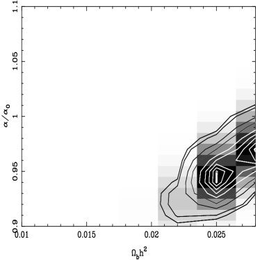
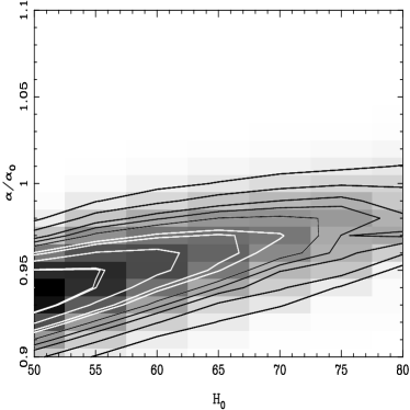
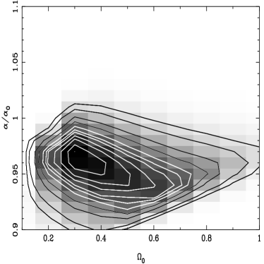
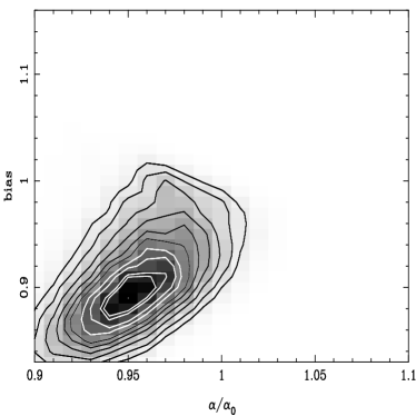
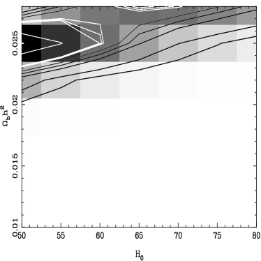
FIG. 5.: Confidence contours for the 2-dim distribution obtained after marginalising over the remaining three parameters (for the calibration nominal case). Contours are at 10,20,30,…90 and 95 per cent confidence levels.

It is of interest to investigate the case where no variation of the fine structure constant is allowed. For that purpose we considered the conditional distribution for $\alpha/\alpha_{0}=1.0$ to obtain a best fit model with

$$H_{0}=75,\quad\Omega_{b}h^{2}=0.028,\quad\Omega_{0}=0.3\,;$$ (20)

$$bias=1.0,\quad\chi^{2}=17.49\,.$$ (21)

In Fig 6 we plot this distribution marginalised over $\Omega_{0}$ and the bias. Increasing the value of $\alpha$ seems to force a higher best fit value of $H_{0}$ and of $\Omega_{b}h^{2}$ and a lower value of $\Omega_{0}$ with a best fit COBE normalised model. Again, this is consistent with [29] (which also find a tilt $n_{s}=0.99$, while [24] find $n_{s}=0.92$).

If we instead condition our distribution to a value of $\Omega_{b}h^{2}=0.019$ we get a best fit model with

$$H_{0}=50,\quad\Omega_{0}=0.3,\quad\alpha/\alpha_{0}=0.9\,;$$ (22)

$$bias=0.89,\quad\chi^{2}=18.23\,.$$ (23)

This result emphasises the rather obvious point that reducing the value of $\Omega_{b}h^{2}$ requires a lower value of $\alpha/\alpha_{0}$ to account for a low second acoustic peak.

Once more, we emphasise that the values of $\Omega_{b}$ are obtained as function of $H_{0}$ in order to satisfy the range for $\Omega_{b}h^{2}$ defined above. This means that we should expect to observe some correlation when plotting $H_{0}$ against $\Omega_{b}h^{2}$. This is indeed confirmed by Fig 3.

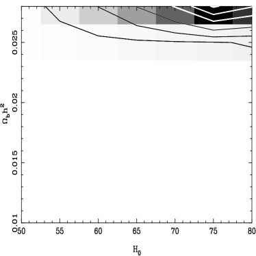
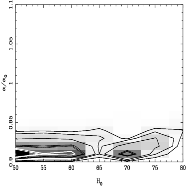
FIG. 6.: Confidence contours for the 2-dim distribution of ($H_{0}$, $\Omega_{b}h^{2}$); marginalised over the remaining parameters (left hand side plot) ; conditional distribution for $\alpha/\alpha_{0}=1$ and marginalised over the remaining parameters (right hand side plot). Bottom plot: Confidence contours for the 2-dim distribution of ($\alpha/\alpha_{0}$,$H_{0}$) conditional to $\Omega_{b}h^{2}=0.019$ and marginalised over the remaining parameters (for the calibration corrected likelihood). Contours are at 10,20,30,…90 and 95 per cent confidence levels.

Therefore we have so far confirmed the fact that to fit a low second Doppler peak we need a high baryonic content [31, 30] and a lower fine structure constant in the past. However, an important question still remains: what’s the weight of the second acoustic peak relative to the main peak in drawing the above conclusions? We recall that in [12] it was shown that the position of the first Doppler peak can by itself provide a constraint on $\alpha$. Can it happen that the main acoustic peak is still a heavy factor in determining the above best fit parameters?

B The first Doppler peak

In order to answer this important question, we considered the set of data points sampling the multi-pole region to up $l\sim 400$. Hence this data set consists now on the first 8 Boomerang and the first 5 Maxima data points with the nominal calibration ($BM_{dp}$). We then repeat the likelihood analysis for this new data set.

We obtain a best fit model with

$$H_{0}=50,\quad\Omega_{b}h^{2}=0.019,\quad\Omega_{0}=0.4\,,$$ (24)

$$\alpha/\alpha_{0}=0.9,\quad bias=0.87,\quad\chi^{2}=14.91\,.$$ (25)

This is rather encouraging, particularly because the best-fit value for $\Omega_{b}h^{2}$ is precisely the one found by observations. However, the maxima and confidence intervals for the marginalised distributions are as follows (again, all are $1\sigma$): $\alpha/\alpha_{0}=0.97\pm 0.04$, $H_{0}=71.4^{+6.1}_{-13.5}$; $\Omega_{b}h^{2}=0.024\pm 0.003$, $\Omega_{0}=0.4^{+0.37}_{-0.21}$, $bias=1.0^{+0.05}_{-0.08}$.

We conclude that most of the best fit model parameters do not lay within the $1\sigma$ range around the maximum of the marginalised distribution for the corresponding parameter. Therefore the 5-dim likelihood must have a narrow peak around this best model with an enlarged surface around the remaining values which height is not significantly smaller then the absolute peak.

In Fig 7 we plot the marginalised distributions for all the parameters, while in fig 8 we plot the 2-dim Likelihood functions obtained after marginalising over the remaining three parameters.

FIG. 7.: Marginal distributions for each model parameter for a subsection of data probing the main doppler peak region (and nominal calibration case) ($BM_{dp}$).

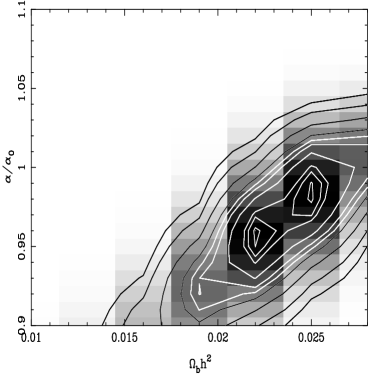
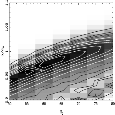
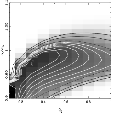
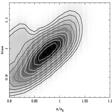
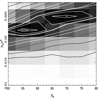
FIG. 8.: Confidence contours for the 2-dim distribution obtained after marginalising over the remaining three parameters for $BM_{dp}$. Contours are at 10,20,30,…90 and 95 per cent confidence levels.

Comparing Fig 7 with Fig 1 we immediately notice a number of extremely interesting points. Firstly, even though the dataset for the first Doppler peak favours a smaller $\alpha$ in the past, there is a non-negligible likelihood for larger values as well. The inclusion of information from the second Doppler peak all but eliminates this possibility (compare this with Fig. 4 of [24]). Secondly, the full dataset increases the preferred values of $\Omega_{b}h^{2}$ (or more accurately, decreases the probability for low values). And thirdly, data from the first Doppler peak alone is basically insensitive to $H_{0}$ and $\Omega_{0}$ (recall that all our models have $\Omega_{total}=1$), while the full dataset tends to favour low values of $H_{0}$ and also narrows the distribution for $\Omega_{0}$ around a value of $\Omega_{0}=0.3$ (and most notably reduces the probability of lower values such as $\Omega_{0}=0.1$ which would be allowed by the reduced dataset).

This might explain the differences in the contour plots of the 2-dim distribution of ($\alpha/\alpha_{0}$, $\Omega_{0}$) in Fig 8 and Fig 5; the plot in Fig 8 shows a correlation between ($\alpha/\alpha_{0}$, $\Omega_{0}$) which disappears when including the other Doppler peaks. These 2-dim plots do also indicate correlations between ($\alpha/\alpha_{0}$, $H_{0}$); ($\alpha/\alpha_{0}$,$\Omega_{b}h^{2}$) and ($\alpha/\alpha_{0}$,bias) which do exist in both situations.

Finally, we also consider the case with no variation of the fine structure constant allowed for the reduced dataset. We obtain a best fit model with

$$H_{0}=75,\quad\Omega_{b}h^{2}=0.025,\quad\Omega_{0}=0.5\,;$$ (26)

$$bias=1.02,\quad\chi^{2}=15.24\,.$$ (27)

If now we condition our distribution to a value of $\Omega_{b}h^{2}=0.019$ we get a best fit model with

$$H_{0}=50,\quad\Omega_{0}=0.4,\quad\alpha/\alpha_{0}=0.9\,;$$ (28)

$$bias=0.87,\quad\chi^{2}=14.91\,.$$ (29)

In Fig 9 we plot these conditional distributions marginalised over $\Omega_{0}$ and the bias.

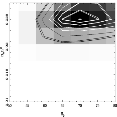
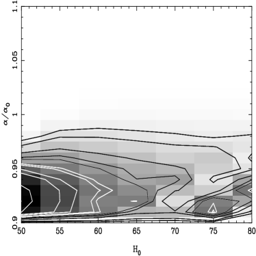
FIG. 9.: Confidence contours for the 2-dim distribution of ($H_{0}$, $\Omega_{b}h^{2}$); marginalised over the remaining parameters (left hand side plot) ; conditional distribution for $\alpha/\alpha_{0}=1$ and marginalised over the remaining parameters (right hand side plot). Bottom plot: Confidence contours for the 2dim distribution of ($\alpha/\alpha_{0}$,$H_{0}$) conditional to $\Omega_{b}h^{2}=0.019$ and marginalised over the remaining parameters (for $BM_{dp}$). Contours are at 10,20,30,…90 and 95 per cent confidence levels.

III Discussion and conclusions

In this paper we have performed a likelihood analysis of the combined BOOMERanG and MAXIMA datasets, allowing for the possibility of a time-varying fine-structure constant, for which there is further observational evidence elsewhere [18, 19]. We have confirmed the intuitively obvious expectation that this data prefers a value of $\alpha$ that was smaller in the past by a few per cent.

However, we wish to emphasise that this is not the same as saying that the CMB can readily provide and unambiguous measurement of the fine-structure constant. As we hopefully made clear above, there are some interesting degeneracies in the problem which imply that other cosmological parameters could still fairly easily mimic a varying $\alpha$. Hence this method of measurement of $\alpha$ is still far from being ‘competitive’, in the sense that statements about $\alpha$ will not be possible until independent accurate determinations of $\Omega_{b}h^{2}$ and $H_{0}$ (and possibly other parameters) are available.

We have also shown that the main reason behind the preferred lower value of $\alpha$ in the present dataset still comes mainly from the data points around the first Doppler peak. The main effect of the high-$\ell$ data points is to increase the preferred value for $\Omega_{b}h^{2}$ and eliminate the possibility of a larger fine-structure constant in the past. A secondary (from this perspective) effect of the small angular scale data is to tighten the constraints on other parameters. Furthermore, we believe that this relative dominance of the low-$\ell$ measurements will remain even in the post-MAP era.

- [1] J. Polchinski, String Theory, Cambridge University Press (1998).
- [2] T. Banks, hep-th/9911067 (1999).
- [3] A. Chodos and S. Detweiler, Phys. Rev. D21, 2167 (1980); W.J. Marciano, Phys. Rev. Lett. 52, 489 (1984).
- [4] Y.S Wu and Z.W. Wang, Phys. Rev. Lett. 57, 1978 (1986).
- [5] E. Kiritsis, J.H.E.P. 10, 10 (1999); S.H.S. Alexander, hep-th/9912037 (1999).
- [6] J.W. Moffat, Int. J. Mod. Phys. D2, 351 (1992); J.W. Moffat, astro-ph/9811390 (1998).
- [7] A. Albrecht and J. Magueijo, Phys. Rev. D59, 043516 (1999); J.D. Barrow, Phys. Rev. D59, 043515 (1999); J.D. Barrow and J. Magueijo, Phys. Lett. B443, 104 (1998).
- [8] P.P. Avelino and C.J.A.P. Martins, Phys. Lett. B459, 468 (1999).
- [9] P.P. Avelino and C.J.A.P. Martins, Phys. Rev. Lett. 85, 1370 (2000).
- [10] J.D. Bekenstein, Phys. Rev. D25, 1527 (1982).
- [11] S. Hannestad, Phys. Rev. D60, 023515 (1999); M. Kaplinghat, R.J. Scherrer and M.S. Turner, Phys. Rev. D60, 023516 (1999).
- [12] P.P. Avelino, C.J.A.P. Martins and G. Rocha, Phys. Lett. B483, 210 (2000).
- [13] D.A. Varshalovich, A.Y. Potekhin and A.V. Ivanchik, physics/0004062 (2000).
- [14] J.D. Prestage, R.L. Tjoelker and L. Maleki, Phys. Rev. Lett. 74, 3511 (1995).
- [15] T. Damour and F. Dyson, Nucl. Phys. B480, 37 (1996).
- [16] P.D. Sisterna and H. Vicetich, Phys. Rev. D41, 1034 (1990).
- [17] L. Bergstrom, S. Iguri and H. Rubinstein, Phys. Rev. D60, 045005 (1999).
- [18] J.K. Webb et al., Phys. Rev. Lett. 82, 884 (1999).
- [19] J.K. Webb et al., seminar at IoA, Cambridge, May 2000.
- [20] P. de Bernardis et al., Nature, 404, 939 (2000).
- [21] A.E. Lange et al., astro-ph/0005004 (2000).
- [22] S. Hanany et al., astro-ph/0005123 (2000).
- [23] A. Balbi et al., astro-ph/0005124 (2000).
- [24] R.A. Battye, R. Crittenden and J. Weller, astro-ph/0008265 (2000).
- [25] S. Hancock, G. Rocha, A.N. Lasenby and C.M. Gutierrez, MNRAS 294L, 1 (1998).
- [26] G. Rocha, in the proceedings of the ‘Early Universe and dark Matter Conference’, DARK98 (July 20-25, 1998, Max-Planck Institut, Heidelberg, Germany) (1998).
- [27] S. Seager, D. Sasselov and D. Scott, Astrophys. J. 523, L1 (1999); S. Seager, D. Sasselov and D. Scott, astro-ph/9912182 (1999).
- [28] C.L. Bennett et al., ApJ. 464, L1 (1996).
- [29] A. Jaffe et al., astro-ph/0007333 (2000).
- [30] M. White, D. Scott and E. Pierpaoli, astro-ph/0004385 (2000).
- [31] W. Hu and N. Sugiyama, Astrophys. J. 444, 489 (1995); W. Hu and N. Sugiyama, Phys. Rev. D51, 2599 (1995).