Particle and Astrophysics Aspects of Ultrahigh Energy Cosmic Rays
Abstract
The origin of cosmic rays is one of the major unresolved astrophysical questions. In particular, the highest energy cosmic rays observed possess macroscopic energies and their origin is likely to be associated with the most energetic processes in the Universe. Their existence triggered a flurry of theoretical explanations ranging from conventional shock acceleration to particle physics beyond the Standard Model and processes taking place at the earliest moments of our Universe. Furthermore, many new experimental activities promise a strong increase of statistics at the highest energies and a combination with ray and neutrino astrophysics will put strong constraints on these theoretical models. Detailed Monte Carlo simulations indicate that charged ultra-high energy cosmic rays can also be used as probes of large scale magnetic fields whose origin may open another window into the very early Universe. We give an overview over this quickly evolving research field.
Keywords: Ultra-High Energy Cosmic Rays
PACS numbers:
1 Introduction
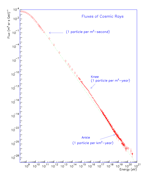
After almost 90 years of research on cosmic rays (CRs), their origin is still an open question, for which the degree of uncertainty increases with energy: Only below 100 MeV kinetic energy, where the solar wind shields protons coming from outside the solar system, the sun must give rise to the observed proton flux. The bulk of the CRs up to at least an energy of eV is believed to originate within our Galaxy. Above that energy, which is associated with the so called “knee”, the flux of particles per area, time, solid angle, and energy, which can be well approximated by broken power laws , steepens from a power law index to one of index . Above the so called “ankle” at eV, the spectrum flattens again to a power law of index . This latter feature is often interpreted as a cross over from a steeper Galactic component to a harder component of extragalactic origin. Fig. 1 shows the measured CR spectrum above 100 MeV, up to eV, the highest energy measured so far for an individual CR.
The conventional scenario assumes that all high energy charged particles are accelerated in magnetized astrophysical shocks, whose size and typical magnetic field strength determines the maximal achievable energy, similar to the situation in man made particle accelerators. The most likely astrophysical accelerators for CR up to the knee, and possibly up to the ankle are the shocks associated with remnants of past Galactic supernova explosions, whereas for the presumed extragalactic component powerful objects such as active galactic nuclei are envisaged.

The main focus of this contribution will be on ultrahigh energy cosmic rays (UHECRs), those with energy eV [2, 3, 4, 7, 8, 9], see Fig. 2. For more details on CRs in general the reader is referred to recent monographs [11, 12]. In particular, extremely high energy (EHE)111We shall use the abbreviation EHE to specifically denote energies eV, while the abbreviation UHE for “Ultra-High Energy” will sometimes be used to denote 1 EeV, where 1 EeV = eV. Clearly UHE includes EHE but not vice versa. cosmic rays pose a serious challenge for conventional theories of CR origin based on acceleration of charged particles in powerful astrophysical objects. The question of the origin of these EHECRs is, therefore, currently a subject of much intense debate and discussions as well as experimental efforts; see Refs. [5, 6, 13], and Ref. [10, 14] for recent brief reviews, and Ref. [15] for a detailed review. In Sect. 2 we will summarize detection techniques and present and future experimental projects.
The current theories of origin of EHECRs can be broadly categorized into two distinct “scenarios”: the “bottom-up” acceleration scenario, and the “top-down” decay scenario, with various different models within each scenario. As the names suggest, the two scenarios are in a sense exact opposite of each other. The bottom-up scenario is just an extension of the conventional shock acceleration scenario in which charged particles are accelerated from lower energies to the requisite high energies in certain special astrophysical environments. On the other hand, in the top-down scenario, the energetic particles arise simply from decay of certain sufficiently massive particles originating from physical processes in the early Universe, and no acceleration mechanism is needed.
The problems encountered in trying to explain EHECRs in terms of acceleration mechanisms have been well-documented in a number of studies; see, e.g., Refs. [16, 17, 18]. Even if it is possible, in principle, to accelerate particles to EHECR energies of order 100 EeV in some astrophysical sources, it is generally extremely difficult in most cases to get the particles come out of the dense regions in and/or around the sources without losing much energy. Currently, the most favorable sources in this regard are perhaps a class of powerful radio galaxies (see, e.g., Refs. [19, 20] for recent reviews and references to the literature), although the values of the relevant parameters required for acceleration to energies 100 EeV are somewhat on the extreme side [18]. However, even if the requirements of energetics are met, the main problem with radio galaxies as sources of EHECRs is that most of them seem to lie at large cosmological distances, 100 Mpc, from Earth. This is a major problem if EHECR particles are conventional particles such as nucleons or heavy nuclei. The reason is that nucleons above 70 EeV lose energy drastically during their propagation from the source to Earth due to the Greisen-Zatsepin-Kuzmin (GZK) effect [21, 22], namely, photo-production of pions when the nucleons collide with photons of the cosmic microwave background (CMB), the mean-free path for which is few Mpc [23]. This process limits the possible distance of any source of EHE nucleons to 100 Mpc. If the particles were heavy nuclei, they would be photo-disintegrated [24, 25] in the CMB and infrared (IR) background within similar distances. Thus, nucleons or heavy nuclei originating in distant radio galaxies are unlikely to survive with EHECR energies at Earth with any significant flux, even if they were accelerated to energies of order 100 EeV at source. In addition, if cosmic magnetic fields are not close to existing upper limits, EHECRs are not likely to be deflected strongly by large scale cosmological and/or Galactic magnetic fields Thus, EHECR arrival directions should point back to their sources in the sky (see Sect. 5 for details) and EHECRs may offer us the unique opportunity of doing charged particle astronomy. Yet, for the observed EHECR events so far, no powerful sources close to the arrival directions of individual events are found within about 100 Mpc [26, 17]. Very recently, it has been suggested by Boldt and Ghosh [27] that particles may be accelerated to energies eV near the event horizons of spinning supermassive black holes associated with presently inactive quasar remnants whose numbers within the local cosmological Universe (i.e., within a GZK distance of order 50 Mpc) may be sufficient to explain the observed EHECR flux. This would solve the problem of absence of suitable currently active sources associated with EHECRs. A detailed model incorporating this suggestion, however, remains to be worked out.
There are, of course, ways to avoid the distance restriction imposed by the GZK effect, provided the problem of energetics is somehow solved separately and provided one allows new physics beyond the Standard Model of particle physics; we shall discuss those suggestions in Sect. 3.
On the other hand, in the top-down scenario, which will be discussed in Sect. 4, the problem of energetics is trivially solved from the beginning. Here, the EHECR particles owe their origin to decay of some supermassive “X” particles of mass eV, so that their decay products, envisaged as the EHECR particles, can have energies all the way up to . Thus, no acceleration mechanism is needed. The sources of the massive X particles could be topological defects such as cosmic strings or magnetic monopoles that could be produced in the early Universe during symmetry-breaking phase transitions envisaged in Grand Unified Theories (GUTs). In an inflationary early Universe, the relevant topological defects could be formed at a phase transition at the end of inflation. Alternatively, the X particles could be certain supermassive metastable relic particles of lifetime comparable to or larger than the age of the Universe, which could be produced in the early Universe through, for example, particle production processes associated with inflation. Absence of nearby powerful astrophysical objects such as AGNs or radio galaxies is not a problem in the top-down scenario because the X particles or their sources need not necessarily be associated with any specific active astrophysical objects. In certain models, the X particles themselves or their sources may be clustered in galactic halos, in which case the dominant contribution to the EHECRs observed at Earth would come from the X particles clustered within our Galactic Halo, for which the GZK restriction on source distance would be of no concern.
By focusing primarily on “non-conventional” scenarios involving new particle physics beyond the electroweak scale, we do not wish to give the wrong impression that these scenarios explain all aspects of EHECRs. In fact, as we shall see below, essentially each of the specific models that have been studied so far has its own peculiar set of problems. Indeed, the main problem of non-astrophysical solutions of the EHECR problem in general is that they are highly model dependent. On the other hand, it is precisely because of this reason that these scenarios are also attractive — they bring in ideas of new physics beyond the Standard Model of particle physics (such as Grand Unification and new interactions beyond the reach of terrestrial accelerators) as well as ideas of early Universe cosmology (such as topological defects and/or massive particle production in inflation) into the realms of EHECRs where these ideas have the potential to be tested by future EHECR experiments.
The physics and astrophysics of UHECRs are intimately linked with the emerging field of neutrino astronomy (for reviews see Refs. [28, 29]) as well as with the already established field of ray astronomy (for reviews see, e.g., Ref. [30]) which in turn are important subdisciplines of particle astrophysics (for a review see, e.g., Ref. [31]). Indeed, as we shall see, all scenarios of UHECR origin, including the top-down models, are severely constrained by neutrino and ray observations and limits. In turn, this linkage has important consequences for theoretical predictions of fluxes of extragalactic neutrinos above a TeV or so whose detection is a major goal of next-generation neutrino telescopes (see Sect. 2): If these neutrinos are produced as secondaries of protons accelerated in astrophysical sources and if these protons are not absorbed in the sources, but rather contribute to the UHECR flux observed, then the energy content in the neutrino flux can not be higher than the one in UHECRs, leading to the so called Waxman Bahcall bound [32, 34]. If one of these assumptions does not apply, such as for acceleration sources that are opaque to nucleons or in the TD scenarios where X particle decays produce much fewer nucleons than rays and neutrinos, the Waxman Bahcall bound does not apply, but the neutrino flux is still constrained by the observed diffuse ray flux in the GeV range (see Sect. 4.4).
Finally, in Sect. 5 we shall discuss how, apart from the unsolved problem of the source mechanism, EHECR observations have the potential to yield important information on Galactic and extragalactic magnetic fields.
2 Present and Future UHE CR and Neutrino Experiments
The CR primaries are shielded by the Earth’s atmosphere and near the ground reveal their existence only by indirect effects such as ionization. Indeed, it was the height dependence of this latter effect which lead to the discovery of CRs by Hess in 1912. Direct observation of CR primaries is only possible from space by flying detectors with balloons or spacecraft. Naturally, such detectors are very limited in size and because the differential CR spectrum is a steeply falling function of energy (see Fig. 1), direct observations run out of statistics typically around a few TeV.
Above TeV, the showers of secondary particles created in the interactions of the primary CR with the atmosphere are extensive enough to be detectable from the ground. In the most traditional technique, charged hadronic particles, as well as electrons and muons in these Extensive Air Showers (EAS) are recorded on the ground [35] with standard instruments such as water Cherenkov detectors used in the old Volcano Ranch [2] and Haverah Park [4] experiments, and scintillation detectors which are used now-a-days. Currently operating ground arrays for UHECR EAS are the Yakutsk experiment in Russia [7] and the Akeno Giant Air Shower Array (AGASA) near Tokyo, Japan, which is the largest one, covering an area of roughly with about 100 detectors mutually separated by about km [9]. The Sydney University Giant Air Shower Recorder (SUGAR) [3] operated until 1979 and was the largest array in the Southern hemisphere. The ground array technique allows one to measure a lateral cross section of the shower profile. The energy of the shower-initiating primary particle is estimated by appropriately parametrizing it in terms of a measurable parameter; traditionally this parameter is taken to be the particle density at 600 m from the shower core, which is found to be quite insensitive to the primary composition and the interaction model used to simulate air showers.
The detection of secondary photons from EAS represents a complementary technique. The experimentally most important light sources are the fluorescence of air nitrogen excited by the charged particles in the EAS and the Cherenkov radiation from the charged particles that travel faster than the speed of light in the atmospheric medium. The first source is practically isotropic whereas the second one produces light strongly concentrated on the surface of a cone around the propagation direction of the charged source. The fluorescence technique can be used equally well for both charged and neutral primaries and was first used by the Fly’s Eye detector [8] and will be part of several future projects on UHECRs (see below). The primary energy can be estimated from the total fluorescence yield. Information on the primary composition is contained in the column depth (measured in g) at which the shower reaches maximal particle density. The average of is related to the primary energy by
| (1) |
Here, is called the elongation rate and is a characteristic energy that depends on the primary composition. Therefore, if and are determined from the longitudinal shower profile measured by the fluorescence detector, then and thus the composition, can be extracted after determining the energy from the total fluorescence yield. Comparison of CR spectra measured with the ground array and the fluorescence technique indicate systematic errors in energy calibration that are generally smaller than 40%. For a more detailed discussion of experimental EAS analysis with the ground array and the fluorescence technique see, e.g., Refs. [36].
As an upscaled version of the old Fly’s Eye Cosmic Ray experiment, the High Resolution Fly’s Eye detector is currently under construction at Utah, USA [38]. Taking into account a duty cycle of about 10% (a fluorescence detector requires clear, moonless nights), the effective aperture of this instrument will be at EeV, on average about 6 times the Fly’s Eye aperture, with a threshold around eV. Another project utilizing the fluorescence technique is the Japanese Telescope Array [39] which is currently in the proposal stage. If approved, its effective aperture will be about 10 times that of Fly’s Eye above eV, and it would also be used as a Cherenkov detector for TeV ray astrophysics. The largest project presently under construction is the Pierre Auger Giant Array Observatory [40] planned for two sites, one in Argentina and another in the USA for maximal sky coverage. Each site will have a ground array. The southern site will have about 1600 particle detectors (separated by 1.5 km each) overlooked by four fluorescence detectors. The ground arrays will have a duty cycle of nearly 100%, leading to an effective aperture about 30 times as large as the AGASA array. The corresponding cosmic ray event rate above eV will be about 50 events per year. About 10% of the events will be detected by both the ground array and the fluorescence component and can be used for cross calibration and detailed EAS studies. The energy threshold will be around eV, with full sensitivity above eV.
Recently NASA initiated a concept study for detecting EAS from space [42, 43] by observing their fluorescence light from an Orbiting Wide-angle Light-collector (OWL). This would provide an increase by another factor in aperture compared to the Pierre Auger Project, corresponding to an event rate of up to a few thousand events per year above eV. Similar concepts such as the Extreme Universe Space Observatory (EUSO) [44] which is part of the AirWatch program [45] and of which a prototype may be tested on the International Space Station are also being discussed. It is possible that the OWL and AirWatch efforts will merge. The energy threshold of such instruments would be between and eV. This technique would be especially suitable for detection of very small event rates such as those caused by UHE neutrinos which would produce deeply penetrating EAS (see Sect. 4.4). For more details on these recent experimental considerations see Ref. [13].
High energy neutrino astronomy is aiming towards a kilometer scale neutrino observatory. The major technique is the optical detection of Cherenkov light emitted by muons created in charged current reactions of neutrinos with nucleons either in water or in ice. The largest pilot experiments representing these two detector media are the now defunct Deep Undersea Muon and Neutrino Detection (DUMAND) experiment [46] in the deep sea near Hawai and the Antarctic Muon And Neutrino Detector Array (AMANDA) experiment [47] in the South Pole ice. Another water based experiment is situated at Lake Baikal [48]. Next generation deep sea projects include the French Astronomy with a Neutrino Telescope and Abyss environmental RESearch (ANTARES) [49] and the underwater Neutrino Experiment SouthwesT Of GReece (NESTOR) project in the Mediterranean [50], whereas ICECUBE [51] represents the planned kilometer scale version of the AMANDA detector. Also under consideration are neutrino detectors utilizing techniques to detect the radio pulse from the electromagnetic showers created by neutrino interactions in ice. This technique could possibly be scaled up to an effective area of and a prototype is represented by the Radio Ice Cherenkov Experiment (RICE) experiment at the South Pole [52]. Neutrinos can also initiate horizontal EAS which can be detected by giant ground arrays such as the Pierre Auger Project [53]. Furthermore, as mentioned above, deeply penetrating EAS could be detected from space by instruments such as the proposed space based AirWatch type detectors [42, 43, 44, 45]. More details and references on neutrino astronomy detectors are contained in Refs. [28, 54], and some recent overviews on neutrino astronomy can be found in Ref. [29].
3 New Primary Particles and New Interactions
A possible way around the problem of missing counterparts within acceleration scenarios is to propose primary particles whose range is not limited by interactions with the CMB. Within the Standard Model the only candidate is the neutrino, whereas in supersymmetric extensions of the Standard Model, new neutral hadronic bound states of light gluinos with quarks and gluons, so-called R-hadrons that are heavier than nucleons, and therefore have a higher GZK threshold, have been suggested [55].
In both the neutrino and new massive neutral hadron scenario the particle propagating over extragalactic distances would have to be produced as a secondary in interactions of a primary proton that is accelerated in a powerful AGN which can, in contrast to the case of EAS induced by nucleons, nuclei, or rays, be located at high redshift. Consequently, these scenarios predict a correlation between primary arrival directions and high redshift sources. In fact, possible evidence for an angular correlation of the five highest energy events with compact radio quasars at redshifts between 0.3 and 2.2 was recently reported [56]. A new analysis with the somewhat larger data set now available does not support significant correlations [57]. This is currently disputed since another group claims to have found a correlation on the 99.9% confidence level [58]. Only a few more events could confirm or rule out the correlation hypothesis. Note that these scenarios would require the primary proton to be accelerated up to eV, demanding a very powerful astrophysical accelerator. On the other hand, a few dozen such exceptional accelerators in the visible Universe may suffice.
3.1 New Neutrino Interactions
Neutrino primaries have the advantage of being well established particles. However, within the Standard Model their interaction cross section with nucleons, whose charged current part can be parametrized by [59]
| (2) |
falls short by about five orders of magnitude to produce ordinary air showers. However, it has been suggested that the neutrino-nucleon cross section, , can be enhanced by new physics beyond the electroweak scale in the center of mass (CM) frame, or above about a PeV in the nucleon rest frame. Neutrino induced air showers may therefore rather directly probe new physics beyond the electroweak scale.
Two major possibilities have been discussed in the literature for which unitarity bounds need not be violated. In the first, a broken SU(3) gauge symmetry dual to the unbroken SU(3) color gauge group of strong interaction is introduced as the “generation symmetry” such that the three generations of leptons and quarks represent the quantum numbers of this generation symmetry. In this scheme, neutrinos can have close to strong interaction cross sections with quarks. In addition, neutrinos can interact coherently with all partons in the nucleon, resulting in an effective cross section comparable to the geometrical nucleon cross section. This model lends itself to experimental verification through shower development altitude statistics [60].
The second possibility consists of a large increase in the number of degrees of freedom above the electroweak scale [61]. A specific implementation of this idea is given in theories with additional large compact dimensions and a quantum gravity scale TeV that has recently received much attention in the literature [62] because it provides an alternative solution (i.e., without supersymmetry) to the hierarchy problem in grand unifications of gauge interactions. The cross sections within such scenarios have not been calculated from first principles yet. Within the field theory approximation which should hold for squared CM energies , the spin 2 character of the graviton predicts [63] For , several arguments based on unitarity within field theory have been put forward. Ref. [63] suggested
| (3) |
where in the last expression we specified to a neutrino of energy hitting a nucleon at rest. A more detailed calculation taking into account scattering on individual partons leads to similar orders of magnitude [64]. Note that a neutrino would typically start to interact in the atmosphere for , i.e. in the case of Eq. (3) for eV, assuming TeV. The neutrino therefore becomes a primary candidate for the observed EHECR events. However, since in a neutral current interaction the neutrino transfers only about of its energy to the shower, the cross section probably has to be at least a few to be consistent with observed showers which start within the first of the atmosphere [65]. A specific signature of this scenario would be the absence of any events above the energy where grows beyond in neutrino telescopes based on ice or water as detector medium [29], and a hardening of the spectrum above this energy in atmospheric detectors such as the Pierre Auger Project [40] and the proposed space based AirWatch type detectors [42, 43, 44, 45]. Furthermore, according to Eq. (3), the average atmospheric column depth of the first interaction point of neutrino induced EAS in this scenario is predicted to depend linearly on energy. This should be easy to distinguish from the logarithmic scaling, Eq. (1), expected for nucleons, nuclei, and rays. To test such scalings one can, for example, take advantage of the fact that the atmosphere provides a detector medium whose column depth increases from towards the zenith to towards horizontal arrival directions. This probes cross sections in the range . Due to the increased Water/ice detectors would probe cross sections in the range [66].
Within string theory, individual amplitudes are expected to be suppressed exponentially above the string scale which for simplicity we assume here to be comparable to . This can be interpreted as a result of the finite spatial extension of the string states. In this case, the neutrino nucleon cross section would be dominated by interactions with the partons carrying a momentum fraction , leading to [67]
This is probably too small to make neutrinos primary candidates for the highest energy showers observed, given the fact that complementary constraints from accelerator experiments result in TeV [68]. On the other hand, in the total cross section amplitude suppression may be compensated by an exponential growth of the level density [61]. It is currently unclear and it may be model dependent which effect dominates. Thus, an experimental detection of the signatures discussed in this section could lead to constraints on some string-inspired models of extra dimensions.
We note in passing that extra dimensions can have other astrophysical ramifications such as energy loss in stellar environments due to emission of real gravitons into the bulk. The strongest resulting lower limits on come from the consideration of cooling of the cores of hot supernovae and read TeV, TeV, TeV, and TeV for , respectively [69]. In addition, implications of extra dimensions for early Universe physics and inflation are increasingly studied in the literature, but much work is left to be done on the intersection of these research domains.
Independent of theoretical arguments, the UHECR data can be used to put constraints on cross sections satisfying . Particles with such cross sections would give rise to horizontal air showers. The Fly’s Eye experiment established an upper limit on horizontal air showers [70]. The non-observation of the neutrino flux expected from pions produced by UHECR interacting with the CMB the results in the limit [66]
| (13) | |||||
| (22) | |||||
| (31) |
where is the average energy fraction of the neutrino deposited into the shower ( for charged current reactions and for neutral current reactions). Expected neutrino fluxes are shown in Fig. 6. The projected sensitivity of future experiments such as the Pierre Auger Observatories and the AirWatch type satellite projects indicate that the cross section limits Eq. (31) could be improved by up to four orders of magnitude, corresponding to one order of magnitude in or .
3.2 Supersymmetric Particles
Light gluinos binding to quarks, anti-quarks and/or gluons can occur in supersymmetric theories involving gauge-mediated supersymmetry (SUSY) breaking [71] where the resulting gluino mass arises dominantly from radiative corrections and can vary between GeV and GeV. In these scenarios, the gluino can be the lightest supersymmetric particle (LSP). There are also arguments against a light quasi-stable gluino [72], mainly based on constraints on the abundance of anomalous heavy isotopes of hydrogen and oxygen which could be formed as bound states of these nuclei and the gluino. Furthermore, accelerator constraints have become quite stringent [73] and seem to be inconsistent with the original scenario from Ref. [55]. However, the scenario with a “tunable” gluino mass [71] still seems possible and suggests either the gluino–gluon bound state , called glueballino , or the isotriplet , called , as the lightest quasi-stable R-hadron. For a summary of scenarios with light gluinos consistent with accelerator constraints see Ref. [74]. The case of a light quasi-stable gluino does not seem to be settled.
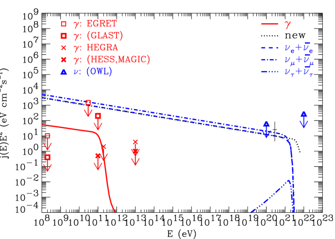
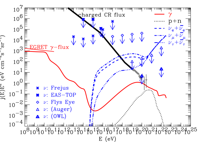
An astrophysical constraint on new neutral massive and strongly interacting EAS primaries results from the fact that the nucleon interactions producing these particles in the source also produce neutrinos and especially rays. The resulting fluxes from powerful discrete acceleration sources may be easily detectable in the GeV range by space-borne ray instruments such as EGRET and GLAST, and in the TeV range by ground based ray detectors such as HEGRA and WHIPPLE and the planned VERITAS, HESS, and MAGIC projects (for reviews discussing these instruments see Ref. [30]). At least the latter three ground based instruments should have energy thresholds low enough to detect rays from the postulated sources at redshift . Such observations in turn imply constraints on the required branching ratio of proton interactions into the R-hadron which, very roughly, should be larger than . These constraints, however, will have to be investigated in more detail for specific sources. One could also search for heavy neutral baryons in the data from Cherenkov instruments in the TeV range in this context. To demonstrate these points, a schematic example of fluxes predicted for the new heavy particle and for rays and neutrinos are shown in Fig. 3.
A further constraint on new EAS primary particles in general comes from the character of the air showers created by them: The observed EHECR air showers are consistent with nucleon primaries and limits the possible primary rest mass to less than GeV [75]. With the statistics expected from upcoming experiments such as the Pierre Auger Project, this upper limit is likely to be lowered down to GeV.
It is interesting to note in this context that in case of a confirmation of the existence of new neutral particles in UHECRs, a combination of accelerator, air shower, and astrophysics data would be highly restrictive in terms of the underlying physics: In the above scenario, for example, the gluino would have to be in a narrow mass range, 1–10 GeV, and the newest accelerator constraints on the Higgs mass, GeV, would require the presence of a D term of an anomalous gauge symmetry, in addition to a gauge-mediated contribution to SUSY breaking at the messenger scale [71].
3.3 Anomalous Kinematics, Quantum Gravity Effects, Lorentz Symmetry Violations
The existence of UHECR beyond the GZK cutoff has prompted several suggestions of possible new physics beyond the Standard Model. We have already discussed some of these suggestions in Sect. 3.1 and 3.2 in the context of new primary particles and new interactions. Further, in Sect. 4 we will discuss suggestions regarding possible new sources of EHECR that also involve postulating new physics beyond the Standard Model. In the present section, to end our discussions on the propagation and new interactions of UHE radiation, we briefly discuss some examples of possible small violations or modifications of certain fundamental tenets of physics (and constraints on the magnitude of those violations/modifications) that have also been discussed in the literature in the context of propagation of UHECR.
For example, as an interesting consequence of the very existence of UHECR, constraints on possible violations of Lorentz invariance (VLI) have been pointed out [76]. These constraints rival precision measurements in the laboratory: If events observed around eV are indeed protons, then the difference between the maximum attainable proton velocity and the speed of light has to be less than about , otherwise the proton would lose its energy by Cherenkov radiation within a few hundred centimeters. Possible tests of other modes of VLI with UHECR have been discussed in Ref. [77], and in Ref. [78] in the context of horizontal air-showers generated by cosmic rays in general. Gonzalez-Mestres [77], Coleman and Glashow [79], and earlier, Sato and Tati [80] and Kirzhnits and Chechin [81] have also suggested that due to modified kinematical constraints the GZK cutoff could even be evaded by allowing a tiny VLI too small to have been detected otherwise. Similar consequences apply to other energy loss processes such as pair production by photons above a TeV with the low energy photon background [82]. It seems to be possible to accomodate such effects within theories involving generalized Lorentz transformations [83] or deformed relativistic kinematics [84]. Furthermore, it has been pointed out [85] that violations of the principle of equivalence (VPE), while not dynamically equivalent, also produce the same kinematical effects as VLI for particle processes in a constant gravitational potential, and so the constraints on VLI from UHECR physics can be translated into constraints on VPE such that the difference between the couplings of protons and photons to gravity must be less than about . Again, this constraint is more stringent by several orders of magnitude than the currently available laboratory constraint from Eötvös experiments.
As a specific example of VLI, we consider an energy dependent photon group velocity where is the speed of light in the low energy limit, , and denotes the energy scale where this modification becomes of order unity. This corresponds to a dispersion relation
| (32) |
which, for example, can occur in quantum gravity and string theory [86]. The kinematics of electron-positron pair production in a head-on collision of a high energy photon of energy with a low energy background photon of energy then leads to the constraint
| (33) |
where and are respectively the energy and outgoing momentum angle (with respect to the original photon momentum) of the electron and positron (). For the case considered by Coleman and Glashow [76] in which the maximum attainable speed of the matter particle is different from the photon speed , the kinematics can be obtained by substituting for in Eq. (33).
Let us define a critical energy TeV in the case of the energy dependent photon group velocity, and in the case considered by Coleman and Glashow. If , or , then becomes negative for . This signals that the photon can spontaneously decay into an electron-positron pair and propagation of photons across extragalactic distances will in general be inhibited. The observation of extragalactic photons up to TeV [87, 88] therefore puts the limits or . In contrast, if , or , will grow with energy for until there is no significant number of target photon density available and the Universe becomes transparent to UHE photons. A clear test of this possibility would be the observation of TeV photons from distances Mps [89]. An unambiguous detection of the thresholds for pion production by nucleons and for pair production by photons in the CMB and other low energy photon backgrounds in the future would allow to establish more stringent lower limits on [90].
In addition, the dispersion relation Eq. (32) implies that a photon signal at energy will be spread out by s. The observation of rays at energies TeV within s from the AGN Markarian 421 therefore puts a limit (independent of ) of GeV, whereas the possible observation of rays at TeV within s from a GRB by HEGRA might be sensitive to [91]. For a recent detailed discussion of these limits see Ref. [92].
A related proposal originally due to Kostelecký in the context of CR suggests the electron neutrino to be a tachyon [93]. This would allow the proton in a nucleus of mass for mass number and charge to decay via above the energy threshold which, for a free proton, is . Ehrlich [94] claims that by choosing it is possible to explain the knee and several other features of the observed CR spectrum, including the high energy end, if certain assumptions about the source distribution are made. The experimental best fit values of from tritium beta decay experiments are indeed negative [95], although this is most likely due to unresolved experimental issues. In addition, the values of from tritium beta decay experiments are typically larger than the value required to fit the knee of the CR spectrum. This scenario also predicts a neutron line around the knee energy [96].
4 Top-Down Scenarios
4.1 The Main Idea
As mentioned in the introduction, all top-down scenarios involve the decay of X particles of mass close to the GUT scale which can basically be produced in two ways: If they are very short lived, as usually expected in many GUTs, they have to be produced continuously. The only way this can be achieved is by emission from topological defects left over from cosmological phase transitions that may have occurred in the early Universe at temperatures close to the GUT scale, possibly during reheating after inflation. Topological defects necessarily occur between regions that are causally disconnected, such that the orientation of the order parameter associated with the phase transition can not be communicated between these regions and consequently will adopt different values. Examples are cosmic strings (similar to vortices in superfluid helium), magnetic monopoles, and domain walls (similar to Bloch walls separating regions of different magnetization in a ferromagnet). The defect density is consequently given by the particle horizon in the early Universe and their formation can even be studied in solid state experiments where the expansion rate of the Universe corresponds to the quenching speed with which the phase transition is induced [97]. The defects are topologically stable, but in the cosmological case time dependent motion leads to the emission of particles with a mass comparable to the temperature at which the phase transition took place. The associated phase transition can also occur during reheating after inflation.
Alternatively, instead of being released from topological defects, X particles may have been produced directly in the early Universe and, due to some unknown symmetries, have a very long lifetime comparable to the age of the Universe. In contrast to Weakly-Interacting Massive Particles (WIMPS) below a few hundred TeV which are the usual dark matter candidates motivated by, for example, supersymmetry and can be produced by thermal freeze out, such superheavy X particles have to be produced non-thermally. Several such mechanisms operating in the post-inflationary epoch in the early Universe have been studied. They include gravitational production through the effect of the expansion of the background metric on the vacuum quantum fluctuations of the X particle field, or creation during reheating at the end of inflation if the X particle field couples to the inflaton field. The latter case can be divided into three subcases, namely “incoherent” production with an abundance proportional to the X particle annihilation cross section, non-adiabatic production in broad parametric resonances with the oscillating inflaton field during preheating (analogous to energy transfer in a system of coupled pendula), and creation in bubble wall collisions if inflation is completed by a first order phase transition. In all these cases, such particles, also called “WIMPZILLAs”, would contribute to the dark matter and their decays could still contribute to UHE CR fluxes today, with an anisotropy pattern that reflects the dark matter distribution in the halo of our Galaxy.
It is interesting to note that one of the prime motivations of the inflationary paradigm was to dilute excessive production of “dangerous relics” such as topological defects and superheavy stable particles. However, such objects can be produced right after inflation during reheating in cosmologically interesting abundances, and with a mass scale roughly given by the inflationary scale which in turn is fixed by the CMB anisotropies to GeV [98]. The reader will realize that this mass scale is somewhat above the highest energies observed in CRs, which implies that the decay products of these primordial relics could well have something to do with EHECRs which in turn can probe such scenarios!
For dimensional reasons the spatially averaged X particle injection rate can only depend on the mass scale and on cosmic time in the combination
| (34) |
where and are dimensionless constants whose value depend on the specific top-down scenario [99], For example, the case is representative of scenarios involving release of X particles from topological defects, such as ordinary cosmic strings [100], necklaces [101] and magnetic monopoles [102]. This can be easily seen as follows: The energy density in a network of defects has to scale roughly as the critical density, , where is cosmic time, otherwise the defects would either start to overclose the Universe, or end up having a negligible contribution to the total energy density. In order to maintain this scaling, the defect network has to release energy with a rate given by , where in the radiation dominated aera, and during matter domination. If most of this energy goes into emission of X particles, then typically . In the numerical simulations presented below, it was assumed that the X particles are nonrelativistic at decay.
The X particles could be gauge bosons, Higgs bosons, superheavy fermions, etc. depending on the specific GUT. They would have a mass comparable to the symmetry breaking scale and would decay into leptons and/or quarks of roughly comparable energy. The quarks interact strongly and hadronize into nucleons (s) and pions, the latter decaying in turn into -rays, electrons, and neutrinos. Given the X particle production rate, , the effective injection spectrum of particle species () via the hadronic channel can be written as , where , and is the relevant fragmentation function (FF).
We adopt the Local Parton Hadron Duality (LPHD) approximation [103] according to which the total hadronic FF, , is taken to be proportional to the spectrum of the partons (quarks/gluons) in the parton cascade (which is initiated by the quark through perturbative QCD processes) after evolving the parton cascade to a stage where the typical transverse momentum transfer in the QCD cascading processes has come down to few hundred MeV, where is a typical hadron size. The parton spectrum is obtained from solutions of the standard QCD evolution equations in modified leading logarithmic approximation (MLLA) which provides good fits to accelerator data at LEP energies [103]. We will specifically use a recently suggested generalization of the MLLA spectrum that includes the effects of supersymmetry [104]. Within the LPHD hypothesis, the pions and nucleons after hadronization have essentially the same spectrum. The LPHD does not, however, fix the relative abundance of pions and nucleons after hadronization. Motivated by accelerator data, we assume the nucleon content of the hadrons to be in the range 3 to 10%, and the rest pions distributed equally among the three charge states. According to recent Monte Carlo simulations [105], the nucleon-to-pion ratio may be significantly higher in certain ranges of values at the extremely high energies of interest here. Unfortunately, however, due to the very nature of these Monte Carlo calculations, it is difficult to understand the precise physical reason for the unexpectedly high baryon yield relative to mesons. While more of these Monte Carlo calculations of the relevant FFs in the future will hopefully clarify the situation, we will use here the range of 3 to 10% mentioned above, which also seems to be supported by other recent Monte Carlo simulations [106]. The standard pion decay spectra then give the injection spectra of -rays, electrons, and neutrinos. For more details concerning uncertainties in the X particle decay spectra see Ref. [107].
4.2 Numerical Simulations
The -rays and electrons produced by X particle decay initiate electromagnetic (EM) cascades on low energy radiation fields such as the CMB. The high energy photons undergo electron-positron pair production (PP; ), and at energies below eV they interact mainly with the universal infrared and optical (IR/O) backgrounds, while above EeV they interact mainly with the universal radio background (URB). In the Klein-Nishina regime, where the CM energy is large compared to the electron mass, one of the outgoing particles usually carries most of the initial energy. This “leading” electron (positron) in turn can transfer almost all of its energy to a background photon via inverse Compton scattering (ICS; ). EM cascades are driven by this cycle of PP and ICS. The energy degradation of the “leading” particle in this cycle is slow, whereas the total number of particles grows exponentially with time. This makes a standard Monte Carlo treatment difficult. Implicit numerical schemes have therefore been used to solve the relevant kinetic equations. A detailed account of the transport equation approach used in the calculations whose results are presented in this contribution can be found in Ref. [108]. All EM interactions that influence the -ray spectrum in the energy range eV, namely PP, ICS, triplet pair production (TPP; ), and double pair production (DPP, ), as well as synchrotron losses of electrons in the large scale extragalactic magnetic field (EGMF), are included.
Similarly to photons, UHE neutrinos give rise to neutrino cascades in the primordial neutrino background via exchange of W and Z bosons [109, 110]. Besides the secondary neutrinos which drive the neutrino cascade, the W and Z decay products include charged leptons and quarks which in turn feed into the EM and hadronic channels. Neutrino interactions become especially significant if the relic neutrinos have masses in the eV range and thus constitute hot dark matter, because the Z boson resonance then occurs at an UHE neutrino energy eV. In fact, this has been proposed as a significant source of EHECRs [111, 112]. Motivated by recent experimental evidence for neutrino mass we assumed a mass of 1 eV for all three neutrino flavors (for simplicity) and implemented the relevant W boson interactions in the t-channel and the Z boson exchange via t- and s-channel. Hot dark matter is also expected to cluster, potentially increasing secondary -ray and nucleon production [111, 112]. This influences mostly scenarios where X decays into neutrinos only. We parametrize massive neutrino clustering by a length scale and an overdensity over the average density . The Fermi distribution with a velocity dispersion yields [114]. Therefore, values of few Mpc and are conceivable on the local Supercluster scale [112].
The relevant nucleon interactions implemented are pair production by protons (), photoproduction of single or multiple pions (, ), and neutron decay. In TD scenarios, the particle injection spectrum is generally dominated by the “primary” -rays and neutrinos over nucleons. These primary -rays and neutrinos are produced by the decay of the primary pions resulting from the hadronization of quarks that come from the decay of the X particles. The contribution of secondary -rays, electrons, and neutrinos from decaying pions that are subsequently produced by the interactions of nucleons with the CMB, is in general negligible compared to that of the primary particles; we nevertheless include the contribution of the secondary particles in our code.
In principle, new interactions such as the ones involving a TeV quantum gravity scale can not only modify the interactions of primary particles in the detector, as discussed in Sect. 3.1, but also their propagation. However, rays and nuclei interact mostly with the CMB and IR for which the CM energy is at most GeV. At such energies the new interactions are much weaker than the dominating electromagnetic and strong interactions. It has been suggested recently [113] that new interactions may notably influence UHE neutrino propagation. However, for neutrinos of mass , the CM energy is GeV, and therefore, UHE neutrino propagation would only be significantly modified for neutrino masses significantly larger than eV. We will therefore ignore this possibility here.
We assume a flat Universe with no cosmological constant, and a Hubble constant of in units of throughout. The numerical calculations follow all produced particles in the EM, hadronic, and neutrino channel, whereas the often-used continuous energy loss (CEL) approximation (e.g., [115]) follows only the leading cascade particles. The CEL approximation can significantly underestimate the cascade flux at lower energies.
The two major uncertainties in the particle transport are the intensity and spectrum of the URB for which there exists only an estimate above a few MHz frequency [116], and the average value of the EGMF. To bracket these uncertainties, simulations have been performed for the observational URB estimate from Ref. [116] that has a low-frequency cutoff at 2 MHz (“minimal”), and the medium and maximal theoretical estimates from Ref. [117], as well as for EGMFs between zero and G, the latter motivated by limits from Faraday rotation measurements, see Sect. 5.2 below. A strong URB tends to suppress the UHE -ray flux by direct absorption whereas a strong EGMF blocks EM cascading (which otherwise develops efficiently especially in a low URB) by synchrotron cooling of the electrons. For the IR/O background we used the most recent data [118].
4.3 Results: ray and Nucleon Fluxes
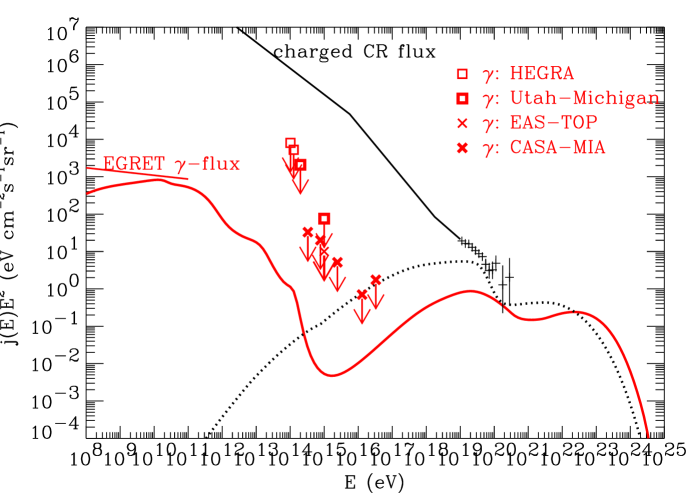
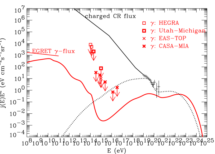
Fig. 4 shows results from Ref. [107] for the time averaged ray and nucleon fluxes in a typical TD scenario, assuming no EGMF, along with current observational constraints on the ray flux. The spectrum was optimally normalized to allow for an explanation of the observed EHECR events, assuming their consistency with a nucleon or ray primary. The flux below eV is presumably due to conventional acceleration in astrophysical sources and was not fit. Similar spectral shapes have been obtained in Ref. [120], where the normalization was chosen to match the observed differential flux at eV. This normalization, however, leads to an overproduction of the integral flux at higher energies, whereas above eV, the fits shown in Figs. 4 and 5 have likelihood significances above 50% (see Ref. [121] for details) and are consistent with the integral flux above eV estimated in Refs. [8, 9]. The PP process on the CMB depletes the photon flux above 100 TeV, and the same process on the IR/O background causes depletion of the photon flux in the range 100 GeV–100 TeV, recycling the absorbed energies to energies below 100 GeV through EM cascading (see Fig. 4). The predicted background is not very sensitive to the specific IR/O background model, however [122]. The scenario in Fig. 4 obviously obeys all current constraints within the normalization ambiguities and is therefore quite viable. Note that the diffuse ray background measured by EGRET [119] up to 10 GeV puts a strong constraint on these scenarios, especially if there is already a significant contribution to this background from conventional sources such as unresolved ray blazars [123]. However, the ray background constraint can be circumvented by assuming that TDs or the decaying long lived X particles do not have a uniform density throughout the Universe but cluster within galaxies [124]. As can also be seen, at energies above 100 GeV, TD models are not significantly constrained by observed ray fluxes yet (see Ref. [15] for more details on these measurements).
Fig. 5 shows results for the same TD scenario as in Fig. 4, but for a high EGMF G, somewhat below the current upper limit, see Eq. (40) below. In this case, rapid synchrotron cooling of the initial cascade pairs quickly transfers energy out of the UHE range. The UHE ray flux then depends mainly on the absorption length due to pair production and is typically much lower [115, 125]. (Note, though, that for eV, the synchrotron radiation from these pairs can be above eV, and the UHE flux is then not as low as one might expect.) We note, however, that the constraints from the EGRET measurements do not change significantly with the EGMF strength as long as the nucleon flux is comparable to the ray flux at the highest energies, as is the case in Figs. 4 and 5. The results of Ref. [107] differ from those of Ref. [120] which obtained more stringent constraints on TD models because of the use of an older fragmentation function from Ref. [126], and a stronger dependence on the EGMF because of the use of a weaker EGMF which lead to a dominance of rays above eV.
The energy loss and absorption lengths for UHE nucleons and photons are short ( Mpc). Thus, their predicted UHE fluxes are independent of cosmological evolution. The ray flux below eV, however, scales as the total X particle energy release integrated over all redshifts and increases with decreasing [127]. For GeV, scenarios with are therefore ruled out (as can be inferred from Figs. 4 and 5), whereas constant comoving injection models () are well within the limits.
We now turn to signatures of TD models at UHE. The full cascade calculations predict ray fluxes below 100 EeV that are a factor and higher than those obtained using the CEL or absorption approximation often used in the literature, in the case of strong and weak URB, respectively. Again, this shows the importance of non-leading particles in the development of unsaturated EM cascades at energies below eV. Our numerical simulations give a /CR flux ratio at eV of . The experimental exposure required to detect a ray flux at that level is , about a factor 10 smaller than the current total experimental exposure. These exposures are well within reach of the Pierre Auger Cosmic Ray Observatories [40], which may be able to detect a neutral CR component down to a level of 1% of the total flux. In contrast, if the EGMF exceeds G, then UHE cascading is inhibited, resulting in a lower UHE ray spectrum. In the G scenario of Fig. 5, the /CR flux ratio at eV is , significantly lower than for no EGMF.
It is clear from the above discussions that the predicted particle fluxes in the TD scenario are currently uncertain to a large extent due to particle physics uncertainties (e.g., mass and decay modes of the X particles, the quark fragmentation function, the nucleon fraction , and so on) as well as astrophysical uncertainties (e.g., strengths of the radio and infrared backgrounds, extragalactic magnetic fields, etc.). More details on the dependence of the predicted UHE particle spectra and composition on these particle physics and astrophysical uncertainties are contained in Ref. [107]. A detailed study of the uncertainties involved in the propagation of UHE nucleons, rays, and neutrinos is currently underway [128].
We stress here that there are viable TD scenarios which predict nucleon fluxes that are comparable to or even higher than the ray flux at all energies, even though rays dominate at production. This occurs, e.g., in the case of high URB and/or for a strong EGMF, and a nucleon fragmentation fraction of ; see, for example, Fig. 5. Some of these TD scenarios would therefore remain viable even if EHECR induced EAS should be proven inconsistent with photon primaries (see, e.g., Ref. [129]). This is in contrast to scenarios with decaying massive dark matter in the Galactic halo which, due to the lack of absorption, predict compositions directly given by the fragmentation function, i.e. domination by rays.
The normalization procedure to the EHECR flux described above imposes the constraint within a factor of a few [120, 107, 130] for the total energy release rate from TDs at the current epoch. In most TD models, because of the unknown values of the parameters involved, it is currently not possible to calculate the exact value of from first principles, although it has been shown that the required values of (in order to explain the EHECR flux) mentioned above are quite possible for certain kinds of TDs. Some cosmic string simulations and the necklace scenario suggest that defects may lose most of their energy in the form of X particles and estimates of this rate have been given [131, 101]. If that is the case, the constraint on translates via Eq. (34) into a limit on the symmetry breaking scale and hence on the mass of the X particle: GeV [132]. Independently of whether or not this scenario explains EHECR, the EGRET measurement of the diffuse GeV ray background leads to a similar bound, , which leaves the bound on and practically unchanged. Furthermore, constraints from limits on CMB distortions and light element abundances from 4He-photodisintegration are comparable to the bound from the directly observed diffuse GeV -rays [127]. That these crude normalizations lead to values of in the right range suggests that defect models require less fine tuning than decay rates in scenarios of metastable massive dark matter.
4.4 Results: Neutrino Fluxes
As discussed in Sect. 4.1, in TD scenarios most of the energy is released in the form of EM particles and neutrinos. If the X particles decay into a quark and a lepton, the quark hadronizes mostly into pions and the ratio of energy release into the neutrino versus EM channel is .
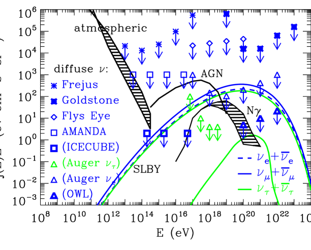
Fig. 6 shows predictions of the total neutrino flux for the same TD model on which Fig. 4 is based. In the absence of neutrino oscillations the electron neutrino and anti-neutrino fluxes are about a factor of 2 smaller than the muon neutrino and anti-neutrino fluxes, whereas the neutrino flux is in general negligible. In contrast, if the interpretation of the atmospheric neutrino deficit in terms of nearly maximal mixing of muon and neutrinos proves correct, the muon neutrino fluxes shown in Fig. 6 would be maximally mixed with the neutrino fluxes. To put the TD component of the neutrino flux in perspective with contributions from other sources, Fig. 6 also shows the atmospheric neutrino flux [135], a typical prediction for the diffuse flux from photon optically thick proton blazars [136] that are not subject to the Waxman Bahcall bound and were normalized to recent estimates of the blazar contribution to the diffuse ray background [123], and the flux range expected for “cosmogenic” neutrinos created as secondaries from the decay of charged pions produced by UHE nucleons [137]. The TD flux component clearly dominates above eV.
In order to translate neutrino fluxes into event rates, one has to fold in the interaction cross sections with matter. At UHEs these cross sections are not directly accessible to laboratory measurements. Resulting uncertainties therefore translate directly to bounds on neutrino fluxes derived from, for example, the non-detection of UHE muons produced in charged-current interactions. In the following, we will assume the estimate Eq. (2) based on the Standard Model for the charged-current muon-neutrino-nucleon cross section if not indicated otherwise.
For an (energy dependent) ice or water equivalent acceptance (in units of volume times solid angle), one can obtain an approximate expected rate of UHE muons produced by neutrinos with energy , , by multiplying (where is the nucleon density in water) with the integral muon neutrino flux . This can be used to derive upper limits on diffuse neutrino fluxes from a non-detection of muon induced events. Fig. 6 shows bounds obtained from several experiments: The Frejus experiment derived upper bounds for eV from their non-detection of almost horizontal muons with an energy loss inside the detector of more than MeV per radiation length [133]. The EAS-TOP collaboration published two limits from horizontal showers, one in the regime eV, where non-resonant neutrino-nucleon processes dominate, and one at the Glashow resonance which actually only applies to [138]. The Fly’s Eye experiment derived upper bounds for the energy range between eV and eV [70] from the non-observation of deeply penetrating particles. The AKENO group has published an upper bound on the rate of near-horizontal, muon-poor air showers [139]. Horizontal air showers created by electrons, muons or tau leptons that are in turn produced by charged-current reactions of electron, muon or tau neutrinos within the atmosphere have recently also been pointed out as an important method to constrain or measure UHE neutrino fluxes [53] with next generation detectors.
The TD model BHS0 from the early work of Ref. [99] is not only ruled out by the constraints from Sect. 4.3, but also by some of the experimental limits on the UHE neutrino flux, as can be seen in Fig. 6. Further, although both the BHS1 and the SLBY98 models correspond to , the UHE neutrino flux above eV in the latter is almost two orders of magnitude smaller than in the former. The main reason for this is the different flux normalization adopted in the two papers: First, the BHS1 model was obtained by normalizing the predicted proton flux to the observed UHECR flux at eV, whereas in the SLBY98 model the actually “visible” sum of the nucleon and ray fluxes was normalized in an optimal way. Second, the BHS1 assumed a nucleon fraction about a factor 3 smaller [99]. Third, the BHS1 scenario used an older fragmentation function from Ref. [126] which has more power at larger energies. Clearly, the SLBY98 model is not only consistent with the constraints discussed in Sect. 4.3, but also with all existing neutrino flux limits within 2-3 orders of magnitude.
What, then, are the prospects of detecting UHE neutrino fluxes predicted by TD models? In a sr size detector, the SLBY98 scenario from Fig. 6, for example, predicts a muon-neutrino event rate of , and an electron neutrino event rate of above eV, where “backgrounds” from conventional sources should be negligible. Further, the muon-neutrino event rate above 1 PeV should be , which could be interesting if conventional sources produce neutrinos at a much smaller flux level. Of course, above TeV, instruments using ice or water as detector medium, have to look at downward going muon and electron events due to neutrino absorption in the Earth. However, neutrinos obliterate this Earth shadowing effect due to their regeneration from decays [140]. The presence of neutrinos, for example, due to mixing with muon neutrinos, as suggested by recent experimental results from Super-Kamiokande, can therefore lead to an increased upward going event rate [141]. For recent compilations of UHE neutrino flux predictions from astrophysical and TD sources see Refs. [43, 142] and references therein.
For detectors based on the fluorescence technique such as the HiRes [38] and the Telescope Array [39] (see Sect. 2), the sensitivity to UHE neutrinos is often expressed in terms of an effective aperture which is related to by . For the cross section of Eq. (2), the apertures given in Ref. [38] for the HiRes correspond to for eV for muon neutrinos. The expected acceptance of the ground array component of the Pierre Auger project for horizontal UHE neutrino induced events is and [53], with a duty cycle close to 100%. We conclude that detection of neutrino fluxes predicted by scenarios such as the SLBY98 scenario shown in Fig. 6 requires running a detector of acceptance over a period of a few years. Apart from optical detection in air, water, or ice, other methods such as acoustical and radio detection [28] (see, e.g., the RICE project [52] for the latter) or even detection from space [42, 43, 44, 45] appear to be interesting possibilities for detection concepts operating at such scales (see Sect. 2). For example, the space based OWL/AirWatch satellite concept would have an aperture of in the atmosphere, corresponding to for eV, with a duty cycle of [42, 43]. The backgrounds seem to be in general negligible [110, 143]. As indicated by the numbers above and by the projected sensitivities shown in Fig. 6, the Pierre Auger Project and especially the space based AirWatch type projects should be capable of detecting typical TD neutrino fluxes. This applies to any detector of acceptance . Furthermore, a 100 day search with a radio telescope of the NASA Goldstone type for pulsed radio emission from cascades induced by neutrinos or cosmic rays in the lunar regolith could reach a sensitivity comparable or better to the Pierre Auger sensitivity above eV [134].
A more model independent estimate [130] for the average event rate can be made if the underlying scenario is consistent with observational nucleon and ray fluxes and the bulk of the energy is released above the PP threshold on the CMB. Let us assume that the ratio of energy injected into the neutrino versus EM channel is a constant . As discussed in Sect. 4.3, cascading effectively reprocesses most of the injected EM energy into low energy photons whose spectrum peaks at GeV [122]. Since the ratio remains roughly unchanged during propagation, the height of the corresponding peak in the neutrino spectrum should roughly be times the height of the low-energy ray peak, i.e., we have the condition Imposing the observational upper limit on the diffuse ray flux around GeV shown in Fig. 6, , then bounds the average diffuse neutrino rate above PP threshold on the CMB, giving
| (35) |
For this bound is consistent with the flux bounds shown in Fig. 6 that are dominated by the Fly’s Eye constraint at UHE. We stress again that TD models are not subject to the Waxman Bahcall bound because the nucleons produced are considerably less abundant than and are not the primaries of produced rays and neutrinos.
In typical TD models such as the one discussed above where primary neutrinos are produced by pion decay, . However, in TD scenarios with neutrino fluxes are only limited by the condition that the secondary ray flux produced by neutrino interactions with the relic neutrino background be below the experimental limits. An example for such a scenario is given by X particles exclusively decaying into neutrinos (although this is not very likely in most particle physics models, but see Ref. [107] and Fig. 7 for a scenario involving topological defects and Ref. [145] for a scenario involving decaying superheavy relic particles, both of which explain the observed EHECR events as secondaries of neutrinos interacting with the primordial neutrino background). Such scenarios predict appreciable event rates above eV in a km3 scale detector, but require unrealistically strong clustering of relic neutrinos (a homogeneous relic neutrino overdensity would make the EGRET constraint only more severe because neutrino interactions beyond Mpc contribute to the GeV ray background but not to the UHECR flux). A detection would thus open the exciting possibility to establish an experimental lower limit on . Being based solely on energy conservation, Eq. (35) holds regardless of whether or not the underlying TD mechanism explains the observed EHECR events.
The transient neutrino event rate could be much higher than Eq. (35) in the direction to discrete sources which emit particles in bursts. Corresponding pulses in the EHE nucleon and ray fluxes would only occur for sources nearer than Mpc and, in case of protons, would be delayed and dispersed by deflection in Galactic and extragalactic magnetic fields [146, 147]. The recent observation of a possible clustering of CRs above eV by the AGASA experiment [148] might suggest sources which burst on a time scale yr. A burst fluence of neutrino induced events within a time could then be expected. Associated pulses could also be observable in the ray flux if the EGMF is smaller than G in a significant fraction of extragalactic space [149].
In contrast to roughly homogeneous sources and/or mechanisms with branching ratios , in scenarios involving clustered sources such as metastable superheavy relic particles decaying with , the neutrino flux is comparable to (not significantly larger than) the UHE photon plus nucleon fluxes. This can be understood because the neutrino flux is dominated by the extragalactic contribution which scales with the extragalactic nucleon and ray contribution in exactly the same way as in the unclustered case, whereas the extragalactic contribution to the “visible” flux to be normalized to the UHECR data is much smaller in the clustered case. The resulting neutrino fluxes would be hardly detectable even with next generation experiments.
5 UHE Cosmic Rays and Cosmological Large Scale Magnetic Fields
5.1 Deflection and Delay of Charged Hadrons
Whereas for UHE electrons the dominant influence of large scale magnetic fields is synchrotron loss rather than deflection, for charged hadrons the opposite is the case. A relativistic particle of charge and energy has a gyroradius where is the field component perpendicular to the particle momentum. If this field is constant over a distance , this leads to a deflection angle
| (36) |
Magnetic fields beyond the Galactic disk are poorly known and include a possible extended field in the halo of our Galaxy and a large scale EGMF. In both cases, the magnetic field is often characterized by an r.m.s. strength and a correlation length , i.e. it is assumed that its power spectrum has a cut-off in wavenumber space at and in real space it is smooth on scales below . If we neglect energy loss processes for the moment, then the r.m.s. deflection angle over a distance in such a field is , or
| (37) |
for , where the numerical prefactors were calculated from the analytical treatment in Ref. [146]. There it was also pointed out that there are two different limits to distinguish: For , particles of all energies “see” the same magnetic field realization during their propagation from a discrete source to the observer. In this case, Eq. (37) gives the typical coherent deflection from the line-of-sight source direction, and the spread in arrival directions of particles of different energies is much smaller. In contrast, for , the image of the source is washed out over a typical angular extent again given by Eq. (37), but in this case it is centered on the true source direction. If , the source may even have several images, similar to the case of gravitational lensing. Therefore, observing images of UHECR sources and identifying counterparts in other wavelengths would allow one to distinguish these limits and thus obtain information on cosmic magnetic fields. If is comparable to or larger than the interaction length for stochastic energy loss due to photo-pion production or photodisintegration, the spread in deflection angles is always comparable to the average deflection angle.
Deflection also implies an average time delay of , or
| (38) |
relative to rectilinear propagation with the speed of light. It was pointed out in Ref. [150] that, as a consequence, the observed UHECR spectrum of a bursting source at a given time can be different from its long-time average and would typically peak around an energy , given by equating with the time of observation relative to the time of arrival for vanishing time delay. Higher energy particles would have passed the observer already, whereas lower energy particles would not have arrived yet. Similarly to the behavior of deflection angles, the width of the spectrum around would be much smaller than if both is smaller than the interaction length for stochastic energy loss and . In all other cases the width would be comparable to .
Constraints on magnetic fields from deflection and time delay cannot be studied separately from the characteristics of the “probes”, namely the UHECR sources, at least as long as their nature is unknown. An approach to the general case is discussed in Sect. 5.3.
5.2 Constraints on EHECR Source Locations
As pointed out in Sect. 1, nucleons, nuclei, and rays above a few eV cannot have originated much further away than Mpc. Together with Eq. (37) this implies that above a few eV the arrival direction of such particles should in general point back to their source within a few degrees [17]. This argument is often made in the literature and follows from the Faraday rotation bound on the EGMF and a possible extended field in the halo of our Galaxy, which in its historical form reads [151], as well as from the known strength and scale height of the field in the disk of our Galaxy, G, kpc. Furthermore, the deflection in the disk of our Galaxy can be corrected for in order to reconstruct the extragalactic arrival direction: Maps of such corrections as a function of arrival direction have been calculated in Refs. [152] for plausible models of the Galactic magnetic field. The deflection of UHECR trajectories in the Galactic magnetic field may, however, also give rise to several other important effects [153] such as (de)magnification of the UHECR fluxes due to the magnetic lensing effect mentioned in the previous section (which can modify the UHECR spectrum from individual sources), formation of multiple images of a source, and apparent “blindness” of the Earth towards certain regions of the sky with regard to UHECRs. These effects may in turn have important implications for UHECR source locations. In fact, it was recently claimed [154] that, assuming a certain model of the magnetic fields in the galactic winds, the highest energy cosmic ray events could all have originated in the Virgo cluster or specifically in the radio galaxy M87. However, as was subsequently pointed out in Ref. [155], this galactic wind model leads to focusing of all positively charged highest energy particles to the North galactic pole and, consequently, this can not be interpreted as evidence for a point source situated close to the North galactic pole.
However, important modifications of the Faraday rotation bound on the EGMF have recently been discussed in the literature: The average electron density which enters estimates of the EGMF from rotation measures, can now be more reliably estimated from the baryon density , whereas in the original bound the closure density was used. Assuming an unstructured Universe and results in the much weaker bound [156]
| (39) |
which suggests much stronger deflection. However, taking into account the large scale structure of the Universe in the form of voids, sheets, filaments etc., and assuming flux freezing of the magnetic fields whose strength then approximately scales with the 2/3 power of the local density, leads to more stringent bounds: Using the Lyman forest to model the density distribution yields [156]
| (40) |
for the large scale EGMF for coherence scales between the Hubble scale and 1 Mpc. This estimate is closer to the original Faraday rotation limit. However, in this scenario the maximal fields in the sheets and voids can be as high as a G [157, 156].
Therefore, according to Eq. (37) and (40), deflection of UHECR nucleons is still expected to be on the degree scale if the local large scale structure around the Earth is not strongly magnetized. However, rather strong deflection can occur if the Supergalactic Plane is strongly magnetized, for particles originating in nearby galaxy clusters where magnetic fields can be as high as G [151] (see Sect. 5.3 below) and/or for heavy nuclei such as iron [26]. In this case, magnetic lensing in the EGMF can also play an important role in determining UHECR source locations [158, 159].
5.3 Angle-Energy-Time Images of UHECR Sources
Small Deflection
For small deflection angles and if photo-pion production is important, one has to resort to numerical Monte Carlo simulations in 3 dimensions. Such simulations have been performed in Ref. [160] for the case and in Refs. [147, 161, 162] for the general case.

In Refs. [147, 161, 162] the Monte Carlo simulations were performed in the following way: The magnetic field was represented as a Gaussian random field with zero mean and a power spectrum with for and otherwise, where characterizes the numerical cut-off scale and the r.m.s. strength is . The field is then calculated on a grid in real space via Fourier transformation. For a given magnetic field realization and source, nucleons with a uniform logarithmic distribution of injection energies are propagated between two given points (source and observer) on the grid. This is done by solving the equations of motion in the magnetic field interpolated between the grid points, and subjecting nucleons to stochastic production of pions and (in case of protons) continuous loss of energy due to PP. Upon arrival, injection and detection energy, and time and direction of arrival are recorded. From many (typically 40000) propagated particles, a histogram of average number of particles detected as a function of time and energy of arrival is constructed for any given injection spectrum by weighting the injection energies correspondingly. This histogram can be scaled to any desired total fluence at the detector and, by convolution in time, can be constructed for arbitrary emission time scales of the source. An example for the distribution of arrival times and energies of UHECRs from a bursting source is given in Fig. 8.
We adopt the following notation for the parameters: denotes the time delay due to magnetic deflection at EeV and is given by Eq. (38) in terms of the magnetic field parameters; denotes the emission time scale of the source; yr corresponds to a burst, and yr (roughly speaking) to a continuous source; is the differential index of the injection energy spectrum; denotes the fluence of the source with respect to the detector, i.e., the total number of particles that the detector would detect from the source on an infinite time scale; finally, is the likelihood function of the above parameters.

By putting windows of width equal to the time scale of observation over these histograms one obtains expected distributions of events in energy and time and direction of arrival for a given magnetic field realization, source distance and position, emission time scale, total fluence, and injection spectrum. Examples of the resulting energy spectrum are shown in Fig. 9. By dialing Poisson statistics on such distributions, one can simulate corresponding observable event clusters.
Conversely, for any given real or simulated event cluster, one can construct a likelihood of the observation as a function of the time delay, the emission time scale, the differential injection spectrum index, the fluence, and the distance. In order to do so, and to obtain the maximum of the likelihood, one constructs histograms for many different parameter combinations as described above, randomly puts observing time windows over the histograms, calculates the likelihood function from the part of the histogram within the window and the cluster events, and averages over different window locations and magnetic field realizations.

In Ref. [161] this approach has been applied to and discussed in detail for the three pairs observed by the AGASA experiment [148], under the assumption that all events within a pair were produced by the same discrete source. Although the inferred angle between the momenta of the paired events acquired in the EGMF is several degrees [163], this is not necessarily evidence against a common source, given the uncertainties in the Galactic field and the angular resolution of AGASA which is . As a result of the likelihood analysis, these pairs do not seem to follow a common characteristic; one of them seems to favor a burst, another one seems to be more consistent with a continuously emitting source. The current data, therefore, does not allow one to rule out any of the models of UHECR sources. Furthermore, two of the three pairs are insensitive to the time delay. However, the pair which contains the EeV event seems to significantly favor a comparatively small average time delay, yr, as can be seen from the likelihood function marginalized over and (see Fig. 10). According to Eq. (38) this translates into a tentative bound for the r.m.s. magnetic field, namely,
| (41) |
which also applies to magnetic fields in the halo of our Galaxy if is replaced by the lesser of the source distance and the linear halo extent. If confirmed by future data, this bound would be at least two orders of magnitude more restrictive than the best existing bounds which come from Faraday rotation measurements [see Eq. (40)] and, for a homogeneous EGMF, from CMB anisotropies [164]. UHECRs are therefore at least as sensitive a probe of cosmic magnetic fields as other measures in the range near existing limits such as the polarization [165] and the small scale anisotropy [166] of the CMB.
More generally, confirmation of a clustering of EHECRs would provide significant information on both the nature of the sources and on large-scale magnetic fields [167]. This has been shown quantitatively [162] by applying the hybrid Monte Carlo likelihood analysis discussed above to simulated clusters of a few tens of events as they would be expected from next generation experiments [6] such as the High Resolution Fly’s Eye [38], the Telescope Array [39], and most notably, the Pierre Auger Project [40] (see Sect. 2), provided the clustering recently suggested by the AGASA experiment [148, 168] is real. The proposed AirWatch type satellite observatory concepts [42, 44, 45] might even allow one to detect clusters of hundreds of such events.
Five generic situations of UHECR time-energy images were discussed in Ref. [162], classified according to the values of the time delay induced by the magnetic field, the emission timescale of the source , as compared to the lifetime of the experiment. The likelihood calculated for the simulated clusters in these cases presents different degeneracies between different parameters, which complicates the analysis. As an example, the likelihood is degenerate in the ratios , or , where is the total fluence, and is the spread in arrival time; these ratios represent rates of detection. Another example is given by the degeneracy between the distance and the injection energy spectrum index . Yet another is the ratio , that controls the size of the scatter around the mean of the correlation. Therefore, in most general cases, values for the different parameters cannot be pinned down, and generally, only domains of validity are found. In the following the reconstruction quality of the main parameters considered is summarized.
The distance to the source can be obtained from the pion production signature, above the GZK cut-off, when the emission timescale of the source dominates over the time delay. Since the time delay decreases with increasing energy, the lower the energy , defined by , the higher the accuracy on the distance . The error on is, in the best case, typically a factor 2, for one cluster of events. In this case, where the emission timescale dominates over the time delay at all observable energies, information on the magnetic field is only contained in the angular image, which was not systematically included in the likelihood analysis of Ref. [162] due to computational limits. Qualitatively, the size of the angular image is proportional to , whereas the structure of the image, i.e., the number of separate images, is controlled by the ratio . Finally, in the case when the time delay dominates over the emission timescale, with a time delay shorter than the lifetime of the experiment, one can also estimate the distance with reasonable accuracy.
Some sensitivity to the injection spectrum index exists whenever events are recorded over a sufficiently broad energy range. At least if the distance is known, it is in general comparatively easy to rule out a hard injection spectrum if the actual , but much harder to distinguish between and 2.5.
If the lifetime of the experiment is the largest time scale involved, the strength of the magnetic field can only be obtained from the time-energy image because the angular image will not be resolvable. When the time delay dominates over the emission timescale, and is, at the same time, larger than the lifetime of the experiment, only a lower limit corresponding to this latter timescale, can be placed on the time delay and hence on the strength of the magnetic field. When combined with the Faraday rotation upper limit Eq. (40), this would nonetheless allow one to bracket the r.m.s. magnetic field strength within a few orders of magnitude. In this case also, significant information is contained in the angular image. If the emission time scale is larger then the delay time, the angular image is obviously the only source of information on the magnetic field strength.
The coherence length enters in the ratio that controls the scatter around the mean of the correlation in the time-energy image. It can therefore be estimated from the width of this image, provided the emission timescale is much less than (otherwise the correlation would not be seen), and some prior information on and is available.

An emission timescale much larger than the experimental lifetime may be estimated if a lower cut-off in the spectrum is observable at an energy , indicating that . The latter may, in turn, be estimated from the angular image size via Eq. (38), where the distance can be estimated from the spectrum visible above the GZK cut-off, as discussed above. An example of this scenario is shown in Fig. 11. For angular resolutions , timescales in the range
| (42) |
could be probed. The lower limit follows from the requirement that it should be possible to estimate from , using Eq. (38), otherwise only an upper limit on , corresponding to this same number, would apply. The upper bound in Eq. (42) comes from constraints on maximal time delays in cosmic magnetic fields, such as the Faraday rotation limit in the case of cosmological large-scale field (smaller number) and knowledge on stronger fields associated with the large-scale galaxy structure (larger number). Eq. (42) constitutes an interesting range of emission timescales for many conceivable scenarios of UHECRs. For example, the hot spots in certain powerful radio galaxies that have been suggested as UHECR sources [169], have a size of only several kpc and could have an episodic activity on timescales of yr.
A detailed comparison of analytical estimates for the distributions of time delays, energies, and deflection angles of nucleons in weak random magnetic fields with the results of Monte Carlo simulations has been presented in Ref. [170]. In this work, deflection was simulated by solving a stochastic differential equation and observational consequences for the two major classes of source scenarios, namely continuous and impulsive UHECR production, were discussed. In agreement with earlier work [150] it was pointed out that at least in the impulsive production scenario and for an EGMF in the range G, as required for cosmological GRB sources, there is a typical energy scale eV below which the flux is quasi-steady due to the spread in arrival times, whereas above which the flux is intermittent with only a few sources contributing.
General Case
Unfortunately, neither the diffusive limit nor the limit of nearly rectilinear propagation is likely to be applicable to the propagation of UHECRs around eV in general. This is because in magnetic fields in the range of a few G, values that are realistic for the Supergalactic Plane [157, 156], the gyro radii of charged particles is of the order of a few Mpc which is comparable to the distance to the sources. An accurate, reliable treatment in this regime can only be achieved by numerical simulation.
To this end, the Monte Carlo simulation approach of individual trajectories developed in Refs. [161, 162] has recently been generalized to arbitrary deflections [158]. The Supergalactic Plane was modeled as a sheet with a thickness of a few Mpc and a Gaussian density profile. The same statistical description for the magnetic field was adopted as in Refs. [161, 162], but with a field power law index , representing a turbulent Kolmogorov type spectrum, and weighted with the sheet density profile. It should be mentioned, however, that other spectra, such as the Kraichnan spectrum, corresponding to , are also possible. The largest mode with non-zero power was taken to be the largest turbulent eddy whose size is roughly the sheet thickness. In addition, a coherent field component is allowed that is parallel to the sheet and varies proportional to the density profile.

When CR backreaction on the weakly turbulent magnetic field is neglected, the diffusion coefficient of CR of energy is determined by the magnetic field power on wavelengths comparable to the particle Larmor radius, and can be approximated by
| (43) |
As a consequence, for the Kolmogorov spectrum, in the diffusive regime, where , the diffusion coefficient should scale with energy as for , and as in the so called Bohm diffusion regime,. This should be reflected in the dependence of the time delay on energy : From the rectilinear regime, , hence at the largest energies, where , this should switch to in the regime of Bohm diffusion, and eventually to at the smallest energies, or largest time delays. Indeed, all three regimes can be seen in Fig. 12 which shows an example of the distribution of arrival times and energies of UHECRs from a bursting source.
The numerical results indicate an effective gyroradius that is roughly a factor 10 higher than the analytical estimate, with a correspondingly larger diffusion coefficient compared to Eq. (43). In addition, the fluctuations of the resulting spectra between different magnetic field realizations can be substantial. This is a result of the fact that most of the magnetic field power is on the largest scales where there are the fewest modes. These considerations mean that the applicability of analytical flux estimates of discrete sources in specific magnetic field configurations is rather limited.
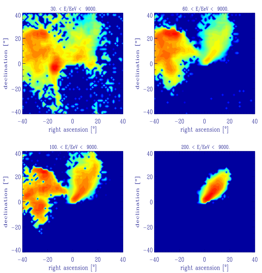
In a steady state situation, diffusion leads to a modification of the injection spectrum by roughly a factor , at least in the absence of significant energy loss and for a homogeneous, infinitely extended medium that can be described by a spatially constant diffusion coefficient. Since in the non-diffusive regime the observed spectrum repeats the shape of the injection spectrum, a change to a flatter observed spectrum at high energies is expected in the transition region [171]. From the spectral point of view this suggests the possibility of explaining the observed UHECR flux above EeV including the highest energy events with only one discrete source [172].
Angular images of discrete sources in a magnetized Supercluster in principle contain information on the magnetic field structure. For the recently suggested field strengths between G and G the angular images are large enough to exploit that information with instruments of angular resolution in the degree range. An example where a transition from several images at low energies to one image at high energies allows one to estimate the magnetic field coherence scale is shown in Fig. 13.
The newest AGASA data [168], however, indicate an isotropic distribution of EHECR. To explain this with only one discrete source would require the magnetic fields to be so strong that the flux beyond eV would most likely be too strongly suppressed by pion production, as discussed above. The recent claim that the powerful radio galaxy Centaurus A at a distance of 3.4 Mpc from Earth can explain both observed flux and angular distributions of UHECRs above eV for an extragalactic magnetic field of strength G [173] was based on the diffusive approximation which is clearly shown by numerical simulations not to apply in this situation; the predicted distributions are too anisotropic even at eV.
This suggests a more continuous source distribution which may also still reproduce the observed UHECR flux above eV with only one spectral component [174]. Statistical studies neglecting magnetic deflection can be performed analytically and also suggest that many sources should contribute to the UHECR spectrum [175]. A more systematic parameter study of sky maps and spectra in UHECR in different scenarios with magnetic fields is now being pursued [176, 159]. Such studies will also be needed to generalize analytical considerations on correlations of UHECR arrival directions with the large scale structure of galaxies [177] to scenarios involving significant magnetic deflection.
Intriguingly, scenarios in which a diffuse source distribution follows the density in the Supergalactic Plane within a certain radius, can accomodate both the large scale isotropy (by diffusion) and the small scale clustering (by magnetic lensing) revealed by AGASA if a magnetic field of strength G permeates the Supercluster [159].
Fig. 14 shows the distribution of arrival times and energies, the solid angle integrated spectrum, and the angular distribution of arrival directions in Galactic coordinates in such a scenario where the UHECR sources with spectral index are distributed according to the matter density in the Local Supercluster, following a pancake profile with scale height of 5 Mpc and scale length 20 Mpc. The r.m.s. magnetic field has a Kolmogorov spectrum with a maximal field strength G in the plane center, and also follows the matter density. The observer is within 2 Mpc of the Supergalactic Plane whose location is indicated by the solid line in the lower panel and at a distance Mpc from the plane center. The absence of sources within 2 Mpc from the observer was assumed. The transition discussed above from the diffusive regime below eV to the regime of almost rectilinear propagation above that energy is clearly visible.
Detailed Monte Carlo simulations performed on these distributions reveal that the anisotropy decreases with increasing magnetic field strength due to diffusion and that small scale clustering increases with coherence and strength of the magnetic field due to magnetic lensing. Both anisotropy and clustering also increase with the (unknown) source distribution radius. Furthermore, the discriminatory power between models with respect to anisotropy and clustering strongly increases with exposure [159].
As a result, a diffuse source distribution associated with the Supergalactic Plane can explain most of the currently observed features of ultra-high energy cosmic rays at least for field strengths close to G. The large-scale anisotropy and the clustering predicted by this scenario will allow strong discrimination against other models with next generation experiments such as the Pierre Auger Project.
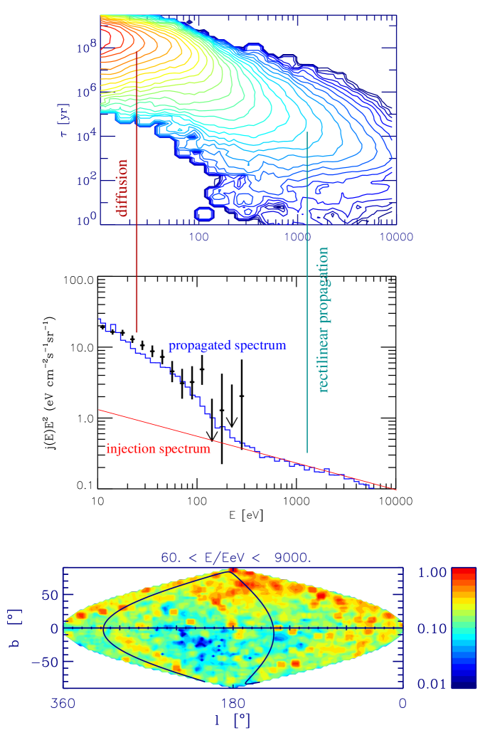
6 Conclusions
Ultra-high energy cosmic rays have the potential to open a window to and act as probes of new particle physics beyond the Standard Model as well as processes occurring in the early Universe at energies close to the Grand Unification scale. Even if their origin will turn out to be attributable to astrophysical shock acceleration with no new physics involved, they will still be witnesses of one of the most energetic processes in the Universe. Furthermore, complementary to other methods such as Faraday rotation measurements, ultra-high energy cosmic rays can be used as probes of the poorly known large scale cosmic magnetic fields. The future appears promising and exciting due to the anticipated arrival of several large scale experiments.
References
- [1] S. Swordy, private communication. The data represent published results of the LEAP, Proton, Akeno, AGASA, Fly’s Eye, Haverah Park, and Yakutsk experiments.
- [2] J. Linsley, Phys. Rev. Lett. 10 (1963) 146; Proc. 8th International Cosmic Ray Conference 4 (1963) 295.
- [3] R. G. Brownlee et al., Can. J. Phys. 46 (1968) S259; M. M. Winn et al., J. Phys. G 12 (1986) 653; see also http://www.physics.usyd.edu.au/hienergy/sugar.html.
- [4] See, e.g., M. A. Lawrence, R. J. O. Reid, and A. A. Watson, J. Phys. G Nucl. Part. Phys. 17 (1991) 733, and references therein; see also http://ast.leeds.ac.uk/haverah/hav-home.html.
- [5] Proc. International Symposium on Astrophysical Aspects of the Most Energetic Cosmic Rays, eds. M. Nagano and F. Takahara (World Scientific, Singapore, 1991)
- [6] Proc. of International Symposium on Extremely High Energy Cosmic Rays: Astrophysics and Future Observatories, ed. M. Nagano (Institute for Cosmic Ray Research, Tokyo, 1996).
- [7] N. N. Efimov et al., Ref. [5], p. 20; B. N. Afnasiev, in Ref. [6], p. 32.
- [8] D. J. Bird et al., Phys. Rev. Lett. 71 (1993) 3401; Astrophys. J. 424 (1994) 491; ibid. 441 (1995) 144.
- [9] N. Hayashida et al., Phys. Rev. Lett. 73 (1994) 3491; S. Yoshida et al., Astropart. Phys. 3 (1995) 105; M. Takeda et al., Phys. Rev. Lett. 81 (1998) 1163; see also http://icrsun.icrr.u-tokyo.ac.jp/as/project/agasa.html.
- [10] M. Nagano, A. A. Watson, Rev. Mod. Phys. 72 (2000) 689.
- [11] V. S. Berezinsky, S. V. Bulanov, V. A. Dogiel, V. L. Ginzburg, and V. S. Ptuskin, Astrophysics of Cosmic Rays (North-Holland, Amsterdam, 1990).
- [12] T. K. Gaisser, Cosmic Rays and Particle Physics, Cambridge University Press (Cambridge, England, 1990)
- [13] Proc. of Workshop on Observing Giant Cosmic Ray Air Showers from eV Particles from Space, eds. J. F. Krizmanic, J. F. Ormes, and R. E. Streitmatter (AIP Conference Proceedings 433, 1997).
- [14] J. W. Cronin, Rev. Mod. Phys. 71 (1999) S165; A. V. Olinto, Phys. Rept. 333-334 (2000) 329; X. Bertou, M. Boratav, and A. Letessier-Selvon, Int. J. Mod. Phys. A15 (2000) 2181; M. Nagano and A. A. Watson, Rev. Mod. Phys. 72 (2000) 689.
- [15] P. Bhattacharjee and G. Sigl, Phys. Rept. 327 (2000) 109.
- [16] A. M. Hillas, Ann. Rev. Astron. Astrophys. 22 (1984) 425.
- [17] G. Sigl, D. N. Schramm, and P. Bhattacharjee, Astropart. Phys. 2 (1994) 401.
- [18] C. A. Norman, D. B. Melrose, and A. Achterberg, Astrophys. J. 454 (1995) 60.
- [19] P. L. Biermann, J. Phys. G: Nucl. Part. Phys. 23 (1997) 1.
- [20] J. G. Kirk and P. Duffy, J. Phys. G: Nucl. Part. Phys. 25 (1999) R163.
- [21] K. Greisen, Phys. Rev. Lett. 16 (1966) 748.
- [22] G. T. Zatsepin and V. A. Kuzmin, Pis’ma Zh. Eksp. Teor. Fiz. 4 (1966) 114 [JETP. Lett. 4 (1966) 78].
- [23] F. W. Stecker, Phys. Rev. Lett. 21 (1968) 1016.
- [24] J. L. Puget, F. W. Stecker, and J. H. Bredekamp, Astrophys. J. 205 (1976) 638.
- [25] L. N. Epele and E. Roulet, Phys. Rev. Lett. 81 (1998) 3295; J. High Energy Phys. 9810 (1998) 009; F. W. Stecker, Phys. Rev. Lett. 81 (1998) 3296; F. W. Stecker and M. H. Salamon, Astrophys. J. 512 (1999) 521.
- [26] J. W. Elbert, and P. Sommers, Astrophys. J. 441 (1995) 151.
- [27] E. Boldt and P. Ghosh, in Mon. Not. R. Astron. Soc. 307 (1999) 491.
- [28] T. K. Gaisser, F. Halzen, and T. Stanev, Phys. Rept. 258 (1995) 173.
- [29] F. Halzen, e-print astro-ph/9810368, lectures presented at the TASI School, July 1998; e-print astro-ph/9904216, talk presented at the 17th International Workshop on Weak Interactions and Neutrinos, Cape Town, South Africa, January 1999;
- [30] R. A. Ong, Phys. Rept. 305 (1998) 95; M. Catanese and T. C. Weekes, e-print astro-ph/9906501, invited review, Publ. Astron. Soc. of the Pacific, Vol. 111, issue 764 (1999) 1193.
- [31] K. Mannheim, Rev. Mod. Astron. 12 (1999) 101.
- [32] E. Waxman and J. Bahcall, Phys. Rev. D. 59 (1999) 023002; J. Bahcall and E. Waxman, e-print hep-ph/9902383.
- [33] Proceedings of the 19th Texas Symposium on Relativistic Astrophysics (Paris, France, 1998).
- [34] K. Mannheim, R. J. Protheroe, and J. P. Rachen, e-print astro-ph/9812398, to appear in Phys. Rev. D.; J. P. Rachen, R. J. Protheroe, and K. Mannheim, e-print astro-ph/9908031, in [33].
- [35] See, e.g., S. Petrera, Nuovo Cimento 19C (1996) 737.
- [36] S. Yoshida and H. Dai, J. Phys. G 24 (1998) 905; P. Sokolsky, Introduction to Ultrahigh Energy Cosmic Ray Physics (Addison Wesley, Redwood City, California, 1989); P. Sokolsky, P. Sommers, and B. R. Dawson, Phys. Rept. 217 (1992) 225; M. V. S. Rao and B. V. Sreekantan, Extensive Air Showers (World Scientific, Singapore, 1998).
- [37] Proc. 24th International Cosmic Ray Conference (Istituto Nazionale Fisica Nucleare, Rome, Italy, 1995)
- [38] S. C. Corbató et al., Nucl. Phys. B (Proc. Suppl.) 28B (1992) 36; D. J. Bird et al., in [37], Vol. 2, 504; Vol. 1,750; M. Al-Seady et al., in [6], p. 191; see also http://hires.physics.utah.edu/.
- [39] M. Teshima et al., Nucl. Phys. B (Proc. Suppl.) 28B (1992), 169; M. Hayashida et al., in [6], p. 205; see also http://www-ta.icrr.u-tokyo.ac.jp/.
- [40] J. W. Cronin, Nucl. Phys. B (Proc. Suppl.) 28B (1992) 213; The Pierre Auger Observatory Design Report (2nd edition), March 1997; see also http://http://www.auger.org/ and http://www-lpnhep.in2p3.fr/auger/welcome.html.
- [41] Proc. 25th International Cosmic Ray Conference, eds.: M. S. Potgieter et al. (Durban, 1997).
- [42] J. F. Ormes et al., in [41], Vol. 5, 273; Y. Takahashi et al., in [6], p. 310; see also http://lheawww.gsfc.nasa.gov/docs/gamcosray/hecr/OWL/.
- [43] D. B. Cline and F. W. Stecker, OWL/AirWatch science white paper, e-print astro-ph/0003459.
- [44] See http://www.ifcai.pa.cnr.it/Ifcai/euso.html.
- [45] J. Linsley, in Ref. [41], Vol. 5, 381; ibid., 385; P. Attinà et al., ibid., 389; J. Forbes et al., ibid., 273; see also http://www.ifcai.pa.cnr.it/Ifcai/airwatch.html.
- [46] See http://dumand.phys.washington.edu/ dumand/.
- [47] For general information see http://amanda.berkeley.edu/; see also F. Halzen, New Astron. Rev 42 (1999) 289.
- [48] For general information see http://www.ifh.de/baikal/baikalhome.html; also see Baikal Collaboration, e-print astro-ph/9906255, talk given at the 8th Int. Workshop on Neutrino Telescopes, Venice, Feb 1999.
- [49] For general information see http://antares.in2p3.fr/antares/antares.html; see also S. Basa, in [33] (e-print astro-ph/9904213); ANTARES Collaboration, e-print astro-ph/9907432.
- [50] For general information see http://www.roma1.infn.it/nestor/nestor.html.
- [51] For general information see http://www.ps.uci.edu/ icecube/workshop.html; see also F. Halzen, Am. Astron. Soc. Meeting 192 (1998) # 62 28; AMANDA collaboration, e-print astro-ph/9906205, talk presented at the 8th Int. Workshop on Neutrino Telescopes, Venice, Feb 1999.
- [52] For general information see http://kuhep4.phsx.ukans.edu/ iceman/index.html.
- [53] J. J. Blanco-Pillado, R. A. Vázquez, and E. Zas, Phys. Rev. Lett. 78 (1997) 3614; K. S. Capelle, J. W. Cronin, G. Parente, and E. Zas, Astropart. Phys. 8 (1998) 321; A. Letessier-Selvon, e-print astro-ph/0009444.
- [54] J. G. Learned, Phil. Trans. Roy. Soc. London A 346 (1994) 99;
- [55] G. R. Farrar, Phys. Rev. Lett. 76 (1996) 4111; D. J. H. Chung, G. R. Farrar, and E. W. Kolb, Phys. Rev. D 57 (1998) 4696;
- [56] G. R. Farrar and P. L. Biermann, Phys. Rev. Lett. 81 (1998) 3579.
- [57] G. Sigl, D. F. Torres, L. A. Anchordoqui, and G. E. Romero, e-print astro-ph/0008363.
- [58] A. Virmani et al., e-print astro-ph/0010235
- [59] R. Gandhi, C. Quigg, M. H. Reno, and I. Sarcevic, Astropart. Phys. 5 (1996) 81; Phys. Rev. D 58 (1998) 093009.
- [60] J. Bordes et al., Astropart. Phys. 8 (1998) 135; in Beyond the Standard Model. From Theory to Experiment (Valencia, Spain, 13-17 October 1997), eds. I. Antoniadis, L. E. Ibanez, and J. W. F. Valle (World Scientific, Singapore, 1998), p. 328 (e-print hep-ph/9711438).
- [61] G. Domokos and S. Kovesi-Domokos, Phys. Rev. Lett. 82 (1999) 1366.
- [62] N. Arkani-Hamed, S. Dimopoulos, and G. Dvali, Phys. Lett. B 429 (1998) 263; I. Antoniadis, N. Arkani-Hamed, S. Dimopoulos, and G. Dvali, Phys. Lett. B 436 (1998) 257; N. Arkani-Hamed, S. Dimopoulos, and G. Dvali, Phys. Rev. D 59 (1999) 086004.
- [63] S. Nussinov and R. Shrock, Phys. Rev. D 59 (1999) 105002.
- [64] P. Jain, D. W. McKay, S. Panda, and J. P. Ralston, Phys. Lett. B484 (2000) 267; J. P. Ralston, P. Jain, D. W. McKay, S. Panda, e-print hep-ph/0008153.
- [65] L. Anchordoqui et al., e-print hep-ph/0011097.
- [66] C. Tyler, A. Olinto, and G. Sigl, e-print hep-ph/0002257, to apprear in Phys. Rev. D.
- [67] M. Kachelrieß and M. Plümacher, Phys. Rev. D 62 (2000) 103006.
- [68] see, e.g., S. Cullen, M. Perelstein, and M. E. Peskin, Phys. Rev.D 62 (2000) 055012, and references therein.
- [69] S. Cullen and M. Perelstein, Phys. Rev. Lett. 83 (1999) 268; V. Barger, T. Han, C. Kao, and R.-J. Zhang, Phys. Lett. B 461 (1999) 34.
- [70] R. M. Baltrusaitis et al., Astrophys. J. 281 (1984) L9; Phys. Rev. D 31 (1985) 2192.
- [71] S. Raby, Phys. Lett. B 422 (1998) 158; S. Raby and K. Tobe, Nucl. Phys. B 539 (1999) 3.
- [72] M. B. Voloshin and L. B. Okun, Sov. J. Nucl. Phys. 43 (1986) 495.
- [73] I. F. Albuquerque et al. (E761 collaboration), Phys. Rev. Lett. 78 (1997) 3252; J. Adams et al. (KTeV Collaboration), Phys. Rev. Lett. 79 (1997) 4083; A. Alavi-Harati et al. (KTeV collaboration), Phys. Rev. Lett. 83 (1999) 2128.
- [74] L. Clavelli, e-print hep-ph/9908342.
- [75] I. F. M. Albuquerque, G. F. Farrar, and E. W. Kolb, Phys. Rev. D 59 (1999) 015021.
- [76] S. Coleman and S. L. Glashow, Phys. Lett. B 405 (1997) 249; Phys. Rev. D 59 (1999) 116008.
- [77] L. Gonzalez-Mestres, Nucl. Phys. B (Proc. Suppl.) 48 (1996) 131; in [13], p. 148.
- [78] R. Cowsik and B. V. Sreekantan, Phys. Lett. B 449 (1999) 219.
- [79] S. Coleman and S. L. Glashow, Nucl. Phys. B574 (2000) 130.
- [80] H. Sato and T. Tati, Prog. Theor. Phys. 47 (1972) 1788.
- [81] D. A. Kirzhnits and V. A. Chechin, Sov. J. Nucl. Phys. 15 (1972) 585.
- [82] T. Kifune, Astrophys. J. 518 (1999) L21.
- [83] G. Yu. Bogoslovsky and H. F. Goenner, Gen. Rel. Grav. 31 (1999) 1565.
- [84] L. Gonzalez-Mestres, e-print hep-ph/9905430, to appear in [144].
- [85] A. Halprin and H. B. Kim, Phys. Lett. B469 (1999) 78.
- [86] see J. Ellis, N. E. Mavromatos, and D. V. Nanopoulos, Gen. Rel. Grav. 31 (1999) 1257, and references therein.
- [87] J. A. Zweerink et al. (WHIPPLE collaboration), Astrophys. J. 490 (1997) L141.
- [88] F. Aharonian et al. (HEGRA collaboration), Astron. Astrophys. 327 (1997) L5.
- [89] W. Kluźniak, e-print astro-ph/9905308, to appear in 8th International Workshop on Neutrino Telescopes, ed. Milla Baldo Ceolin (Venice, 1999); Astropart. Phys. 11 (1999) 117.
- [90] R. Aloisio, P. Blasi, P. L. Ghia, and A. F. Grillo, Phys. Rev. D 62 (2000) 053010.
- [91] see G. Amelino-Camelia et al., Nature 393 (1998) 763, and references therein.
- [92] J. Ellis, K. Farakos, N. E. Mavromatos, V. Mitsou, and D. V. Nanopoulos, Astrophys. J. 535 (2000) 139.
- [93] V. A. Kostelecký, in Topics on Quantum Gravity and Beyond, eds. F. Mansouri and J. J. Scanio (World Scientific, Singapore, 1993).
- [94] R. Ehrlich, Phys. Rev. D 60 (1999) 017302.
- [95] C. Caso et al., European Phys. J. C 3 (1998) 1.
- [96] R. Ehrlich, Phys. Rev. D 60 (1999) 073005.
- [97] see, e.g., T. Vachaspati, Contemp. Phys. 39 (1998) 225.
- [98] for a brief review see V. Kuzmin and I. Tkachev, Phys. Rept. 320 (1999) 199
- [99] P. Bhattacharjee, C. T. Hill, and D. N. Schramm, Phys. Rev. Lett. 69 (1992) 567.
- [100] see, e.g., P. Bhattacharjee and N. C. Rana, Phys. Lett. B 246 (1990) 365.
- [101] V. Berezinsky and A. Vilenkin, Phys. Rev. Lett. 79 (1997) 5202.
- [102] P. Bhattacharjee and G. Sigl, Phys. Rev. D 51 (1995) 4079 .
- [103] Yu. L. Dokshitzer, V. A. Khoze, A. H. Müller, and S. I. Troyan, Basics of Perturbative QCD (Editions Frontieres, Singapore, 1991).
- [104] V. Berezinsky and M. Kachelrieß , Phys. Lett. B 434 (1998) 61.
- [105] M. Birkel and S. Sarkar, Astropart. Phys. 9 (1998) 297; S. Sarkar, e-print hep-ph/0005256, to appear in Proceedings of COSMO-99, Trieste, 27 Sept.-3 Oct. 1999.
- [106] V. Berezinsky and M. Kachelrieß , e-print hep-ph/0009053.
- [107] G. Sigl, S. Lee, P. Bhattacharjee, and S. Yoshida, Phys. Rev. D 59 (1999) 043504.
- [108] S. Lee, Phys. Rev. D 58 (1998) 043004.
- [109] T. J. Weiler, Phys. Rev. Lett. 49 (1982) 234; Astrophys. J. 285 (1984) 495; E. Roulet, Phys. Rev. D 47 (1993) 5247; S. Yoshida, Astropart. Phys. 2 (1994) 187.
- [110] S. Yoshida, H. Dai, C. C. H. Jui, and P. Sommers, Astrophys. J. 479 (1997) 547.
- [111] T. J. Weiler, Astropart. Phys. 11 (1999) 317.
- [112] S. Yoshida, G. Sigl, and S. Lee, Phys. Rev. Lett. 81 (1998) 5505.
- [113] R. V. Konoplich and S. G. Rubin, JETP Lett. 72 (2000) 97, A. Goyal, A. Gupta, and N. Mahajan, e-print hep-ph/0005030.
- [114] see, e.g., P. J. E. Peebles, Principles of Physical Cosmology, Princeton University Press, New Jersey, 1993.
- [115] F. A. Aharonian, P. Bhattacharjee, and D. N. Schramm, Phys. Rev. D 46 (1992) 4188.
- [116] T. A. Clark, L. W. Brown, and J. K. Alexander, Nature 228 (1970) 847.
- [117] R. J. Protheroe and P. L. Biermann, Astropart. Phys. 6 (1996) 45.
- [118] See, e.g., S. Biller et al., Phys. Rev. Lett. 80 (1998) 2992; T. Stanev and A. Franceschini, Astrophys. J. 494 (1998) L159; F. W. Stecker and O. C. de Jager, Astron. Astrophys. 334 (1998) L85.
- [119] P. Sreekumar et al., Astrophys. J. 494 (1998) 523.
- [120] R. J. Protheroe and T. Stanev, Phys. Rev. Lett. 77 (1996) 3708; erratum, ibid. 78 (1997) 3420.
- [121] G. Sigl, S. Lee, D. N. Schramm, and P. Bhattacharjee, Science 270 (1995) 1977.
- [122] P. S. Coppi and F. A. Aharonian, Astrophys. J. 487 (1997) L9.
- [123] R. Mukherjee and J. Chiang, Astropart. Phys. 11 (1999) 213.
- [124] V. Berezinsky, M. Kachelrieß , and A. Vilenkin, Phys. Rev. Lett. 79 (1997) 4302.
- [125] S. Lee, A. V. Olinto, and G. Sigl, Astrophys. J. 455 (1995) L21.
- [126] C. T. Hill, Nucl. Phys. B 224 (1983) 469.
- [127] G. Sigl, K. Jedamzik, D. N. Schramm, and V. Berezinsky, Phys. Rev. D 52 (1995) 6682.
- [128] O. E. Kalashev, V. A. Kuzmin, and D. V. Semikoz, e-print astro-ph/9911035; O. E. Kalashev, V. A. Kuzmin, D. V. Semikoz, and G. Sigl, in preparation.
- [129] F. Halzen, R. V’azques, T. Stanev, and H. P. Vankov, Astropart. Phys. 3 (1995) 151; M. Ave et al., Phys. Rev. Lett. 85 (2000) 2244; E. Zas, e-print astro-ph/0011416.
- [130] G. Sigl, S. Lee, D. N. Schramm, and P. S. Coppi, Phys. Lett. B 392 (1997) 129.
- [131] G. R. Vincent, N. D. Antunes, and M. Hindmarsh, Phys. Rev. Lett. 80 (1998) 2277; G. R. Vincent, M. Hindmarsh, and M. Sakellariadou, Phys. Rev. D 56 (1997) 637.
- [132] U. F. Wichoski, J. H. MacGibbon, and R. H. Brandenberger, e-print hep-ph/9805419, submitted to Phys. Rev. D.
- [133] W. Rhode et al., Astropart. Phys. 4 (1996) 217.
- [134] P. W. Gorham, K. M. Liewer, and C. J. Naudet, e-print astro-ph/9906504, to appear in [144].
- [135] P. Lipari, Astropart. Phys. 1 (1993) 195.
- [136] R. Protheroe, in Accretion Phenomena and Related Outflows, Vol. 163 of IAU Colloquium, eds. D. Wickramasinghe, G. Bicknell, and L. Ferrario (Astron. Soc. of the Pacific, 1997), p. 585.
- [137] R. J. Protheroe and P. A. Johnson, Astropart. Phys. 4 (1996) 253, and erratum ibid. 5 (1996) 215.
- [138] M. Aglietta et al. (EAS-TOP collaboration), in [37], Vol. 1, 638.
- [139] M. Nagano et al., J. Phys. G 12 (1986) 69.
- [140] F. Halzen and D. Saltzberg, Phys. Rev. Lett. 81 (1998) 4305.
- [141] K. Mannheim, Astropart. Phys. 11 (1999) 49.
- [142] R. Protheroe, e-print astro-ph/9809144, invited talk at Neutrino 98, Takayama 4-9 June 1998; M. Roy and H. J. Crawford, e-print astro-ph/9808170, submitted to Astropart. Phys.; R. Ghandi, e-print astro-ph/0011176.
- [143] P. B. Price, Astropart. Phys. 5 (1996) 43.
- [144] Proc. 26th International Cosmic Ray Conference, (Utah, 1999).
- [145] G. Gelmini and A. Kusenko, Phys. Rev. Lett. 84 (2000) 1378; G. Gelmini, e-print hep-ph/0005263, to appear in Proceedings of 4th International Symposium on Sources and Detection of Dark Matter in the Universe, Feb. 2000, Marina del Rey.
- [146] E. Waxman and J. Miralda-Escudé, Astrophys. J. 472 (1996) L89.
- [147] M. Lemoine, G. Sigl, A. V. Olinto, and D.N. Schramm, Astrophys. J., 486 (1997) L115.
- [148] N. Hayashida et al., Phys. Rev. Lett. 77 (1996) 1000.
- [149] E. Waxman and P. S. Coppi, Astrophys. J. 464 (1996) L75.
- [150] J. Miralda-Escudé and E. Waxman, Astrophys. J. 462 (1996) L59.
- [151] P. P. Kronberg, Rep. Prog. Phys. 57 (1994) 325; J. P. Vallée, Fundamentals of Cosmic Physics, Vol. 19 (1997) 1.
- [152] T. Stanev, Astrophys. J. 479 (1997) 290; G. A. Medina Tanco, E. M. de Gouveia Dal Pino, and J. E. Horvath, Astrophys. J. 492 (1998) 200.
- [153] D. Harari, S. Mollerach, and E. Roulet, JHEP 08 (1999) 022; ibid. 0002 (2000) 035; ibid. 0010 (2000) 047.
- [154] E.-J. Ahn, G. Medina-Tanco, P. L. Biermann, and T. Stanev, e-print astro-ph/9911123.
- [155] P. Billoir and A. Letessier-Selvon, e-print astro-ph/0001427.
- [156] P. Blasi, S. Burles, and A. V. Olinto, Astrophys. J. 514 (1999) L79.
- [157] D. Ryu, H. Kang, and P. L. Biermann, Astron. Astrophys. 335 (1998) 19.
- [158] G. Sigl, M. Lemoine, and P. Biermann, Astropart. Phys. 10 (1999) 141.
- [159] M. Lemoine, G. Sigl, and P. Biermann, e-print astro-ph/9903124.
- [160] G. A. Medina Tanco, E. M. de Gouveia Dal Pino, and J. E. Horvath, Astropart. Phys. 6 (1997) 337.
- [161] G. Sigl, M. Lemoine, and A. Olinto, Phys. Rev. D. 56 (1997) 4470.
- [162] G. Sigl and M. Lemoine, Astropart. Phys. 9 (1998) 65.
- [163] G. A. Medina Tanco, Astrophys. J. 495 (1998) L71.
- [164] J. D. Barrow, P. G. Ferreira, and J. Silk, Phys. Rev. Lett. 78 (1997) 3610.
- [165] A. Loeb and A. Kosowsky, Astrophys. J. 469 (1996) 1.
- [166] K. Subramanian and J. D. Barrow, Phys. Rev. Lett. 81 (1998) 3575.
- [167] G. Sigl, D. N. Schramm, S. Lee, and C. T. Hill, Proc. Natl. Acad. Sci. USA, Vol 94 (1997) 10501.
- [168] M. Takeda et al., Astrophys. J. 522 (1999) 225; e-print astro-ph/0008102.
- [169] J. P. Rachen and P. L. Biermann, Astron. Astrophys. 272 (1993) 161.
- [170] A. Achterberg, Y. Gallant, C. A. Norman, and D. B. Melrose, e-print astro-ph/9907060, submitted to Mon. Not. R. Astron. Soc.
- [171] J. Wdowczyk and A. W. Wolfendale, Nature 281 (1979) 356; M. Giler, J. Wdowczyk, and A. W. Wolfendale, J. Phys. G.: Nucl. Phys. 6 (1980) 1561; V. S. Berezinskii, S. I. Grigo’eva, and V. A. Dogiel, Sov. Phys. JETP 69 (1989) 453; G. R. Farrar and T. Piran, Phys.Rev.Lett. 84 (2000) 3527.
- [172] P. Blasi and A. V. Olinto, Phys. Rev. D. 59 (1999) 023001.
- [173] G. R. Farrar and T. Piran, e-print astro-ph/0010370.
- [174] G. Medina Tanco, Astrophys. J. 510 (1999) L91; e-print astro-ph/9905239, to appear in [144].
- [175] S. L. Dubovsky, P. G. Tinyakov, and I. I. Tkachev, Phys.Rev.Lett. 85 (2000) 1154; Z. Fodor and S. D. Katz, e-print hep-ph/0007158.
- [176] G. Medina Tanco, e-print astro-ph/9809219, to appear in Topics in cosmic-ray astrophysics, ed. M. A. DuVernois (Nova Scientific, New York, 1999).
- [177] E. Waxman, K. B. Fisher, and T. Piran, Astrophys. J. 483 (1997) 1; R. Ugoccioni, L. Teodoro, and U. Wichoski, e-print astro-ph/0011171.