Topology of the Galaxy Distribution in the Hubble Deep Fields

Abstract

We have studied topology of the distribution of the high redshift galaxies identified in the Hubble Deep Field (HDF) North and South. The two-dimensional genus is measured from the projected distributions of the HDF galaxies at angular scales from $3.8^{\prime\prime}$ to $6.1^{\prime\prime}$. We have also divided the samples into three redshift slices with roughly equal number of galaxies using photometric redshifts to see possible evolutionary effects on the topology.

The genus curve of the HDF North clearly indicates clustering of galaxies over the Poisson distribution while the clustering is somewhat weaker in the HDF South. This clustering is mainly due to the nearer galaxies in the samples. We have also found that the genus curve of galaxies in the HDF is consistent with the Gaussian random phase distribution with no significant redshift dependence.

1 INTRODUCTION

An important prediction of typical inflationary models is that the matter fluctuation field has a Gaussian random phase distribution. At large linear scales where the galaxy distribution is presumely still in the linear regime and therefore keeping the statistics of the primordial fluctuation field, studies of the topology of the galaxy distribution can test such predictions. At smaller non-linear scales where the galaxy distribution depends sensitively on the small-scale physics, a study of topology can give us information on the mechanism of galaxy formation and evolution as well as on cosmology.

During the past 15 years topology of large scale structures has been measured by many authors using various observational samples following after the initial work of Gott, Melott & Dickinson (1986), Hamilton, Gott & Weinberg (1986), and Gott, Weinberg & Melott (1987). Among these, topology measures for two-dimensional fields have been introduced by Coles & Barrow (1987), Melott et al. (1989) and Gott et al. (1990), and applied to observational samples like the angular distribution of galaxies on the sky (Coles & Plionis 1991; Gott et al. 1992), the distribution of galaxies in slices of the universe (Park et al. 1992; Colley 1997) and the temperature fluctuation field of the Cosmic Microwave Background (Coles 1988; Gott et al. 1990; Smoot et al. 1994; Kogut et al. 1996; Colley, Gott & Park 1996; Park et al. 1998). In the first two cases where the samples dominantly include nearby galaxies, the topology of two-dimensional galaxy distributions as revealed by the genus or the Euler-Poincaré characteristic statistics, is consistent with the random phase Gaussian distribution with a possible weak ‘meat-ball’ topology.

The HDF images (Williams et al. 1996) taken by the Wide Field Planetary Camera 2 (WFPC-2) on the Hubble Space Telescope, have given us an unprecedently deep view of the high redshift universe. One can easily detect objects with AB magnitudes (Oke 1974) down to $28\sim 29$ (Madau et al. 1996) and with an angular resolution of about $0.05^{\prime\prime}$. Important issues one can address from the HDF data include the discovery of proto-galaxies forming at high redshifts, or delineating the epoch of galaxy formation (Steidel et al. 1996; Clements & Couch 1996; Park & Kim 1998). Another important problem one can study from the HDF data is the properties of galaxies at high redshifts, or the evolution of galaxies. This can be done by looking at numbers, colors, and clustering of galaxies as a function of redshift.

In this paper we study the topology of the distribution of galaxies identified in the HDF North and South and having either spectroscopic or photometric redshifts (Fernández-Soto, Lanzetta, & Yahil 1999, hereafter FLY99; Lanzetta et al. 1999). From these data sets we hope to study the topology of the galaxy distribution at high redshifts.

2 Topology Measure

2.1 The Genus

We use the two-dimensional genus statistic introduced by Melott et al. (1989) as a quantitative measure of topology of the galaxy distribution in the HDFs. The study most similar to our work is that of Gott et al. (1992) who have measured the genus of angular distributions of nearby galaxies in the UGC and ESO catalogs. Coles & Plionis (1991) have also measured the Euler-Poincaré characteristic, which is equivalent to the genus in the limit of negligible sample boundary effects, for the Lick catalog.

The two-dimensional genus is defined as (Gott et al. 1992)

$$G={\rm(number\;of\;isolated\;high\;density\;regions)}-{\rm(number\;of\;isolated\;low\;density\;regions)}.$$

When a two-dimensional distribution is given, the Gauss-Bonnett theorem relates the genus of isodensity contours with the line integral of the local curvature $\kappa$ (Gott et al. 1990)

$$G={1\over 2\pi}\int\kappa ds.$$

In the case of a Gaussian random field the genus per unit area is known to be (Melott et al. 1989; Coles 1988)

$$g={1\over(2\pi)^{3/2}}{\langle k^{2}\rangle\over 2}\nu e^{-\nu^{2}/2},$$

where $\nu$ is the threshold density for the isodensity contour in units of standard deviations from the mean, $\langle k^{2}\rangle=\int k^{2}P_{2}(k)d^{2}k/\int P_{2}(k)d^{2}k$ and $P_{2}(k)$ is the smoothed two-dimensional power spectrum. In practice, we are not interested in the one-point distribution of the density field, and therefore use the label $\nu_{A}$ which parametrizes the area faction by

$$f_{\rm A}={1\over\sqrt{2\pi}}\int_{\nu_{A}}^{\infty}e^{-t^{2}/2}dt.$$

We calculate the genus from $\nu_{A}=-3$ to 3 with an interval of 0.2.

When the power spectrum of the three-dimensional galaxy distribution is of the power-law form $P_{3}(k)\propto k^{n}$ and when the thickness of the two-dimensional slice is much larger or smaller than the smoothing length of the Gaussian filter $W(r)\propto e^{-r^{2}/2R_{G}^{2}}$, there exist simple analytic formulae for the amplitude (Melott et al. 1989)

$$\langle k^{2}\rangle={F(n)\over R_{G}^{2}},$$

where $F(n)=(n+2)/2$ for $n>-2$ and $0$ for $-3<n\leq-2$ for slices with thickness much larger than the smoothing length $R_{G}$, and $F(n)=1$ for $n\geq-1$ and $(n+3)/2$ for $-3<n<-1$ for thin slices. The thick slice approximation is relevant for maps of galaxies projected on the sky.

2.2 The Genus-Related statistics

Since the genus-threshold density relation for Gaussian fields is known, non-Gaussian behaviour of a field can be detected from deviations from the relation. We quantify such deviations by genus-related statistics. The first is the shift of the genus curve $\Delta\nu$ (Park et al. 1992). We measure the shift parameter from the observed genus curve by minimizing the $\chi^{2}$ between the data and the fitting function

$$G=A\nu^{\prime}e^{-\nu^{\prime 2}/2},$$

where $\nu^{\prime}=\nu-\Delta\nu$ and the amplitude $A$ of the genus curve is allowed to have different values at negative and positive $\nu^{\prime}$. The $\chi^{2}$-minimization is performed over the range $-1.0\leq\nu\leq 1.0$.

The second statistic is the asymmetry parameter which measures the difference in the amplitude of the genus curve in the positive and negative thresholds (i.e. the difference between the numbers of clumps and voids). The asymmetry parameter is defined as

$$\Delta g=A_{C}-A_{V},$$

where

$$A_{C}=\int_{\nu_{1}}^{\nu_{2}}g_{\rm obs}d\nu/\int_{\nu_{1}}^{\nu_{2}}g_{\rm fit}d\nu,$$

and likewise for $A_{V}$. The integration is limited to $-2\leq\nu\leq-0.4$ for $A_{V}$ and to $0.4\leq\nu\leq 2$ for $A_{C}$. The overall amplitude $A$ of the best-fit genus curve $g_{\rm fit}$ is found from the $\chi^{2}$-fitting over the range $-2.0\leq\nu\leq 2.0$. $\Delta g$ is positive when high-density regions are divided into many clumps while the low-density regions are merged into fewer voids. For an observed genus curve, we therefore measure the best-fit amplitude $A$, the shift parameter $\Delta\nu$, and the asymmetry parameter $\Delta g$.

3 Analysis of the HDF Data

3.1 The HDF data

We use the photometric redshift data of galaxies in the HDF North (hereafter HDFN) published by FLY99. The catalog has 1067 galaxies with photometric and/or spectroscopic redshifts. We use the spectroscopic redshifts whenever available. We limit the sample to $z\leq 2$, which leaves us with 820 galaxies because the redshift space distribution of galaxies sharply drops at $z\sim 2$ and because the photometric redshift starts to have relatively large error at $z\geq 2$ (FLY99). We then drop the Planetary Camera image as well as the edges of the Wide Field Camera images where the magnitude limit to the sample is bright, i.e. $AB(8140)=26.0$.

In Figure 1 the long-dashed lines delineate the inner part of the WFPC2 images which encloses 714 galaxies with $AB(8140)\leq 28.0$ (hereafter the S-zone; see dash lines in Fig. 1 of FLY99). The genus is actually measured in the region 100 pixels inside these boundaries (hereafter the G-zone; thick solid lines in Figure 1) after the galaxy distribution is smoothed in the S-zone. There are 605 galaxies with $z\leq 2$ and $AB(8140)\leq 28.0$ in the G-zone. To see the possible evolution effects we divide the HDFN sample into three overlapping redshift slice subsamples, each of which contains about 300 galaxies in the G-zone. Table 1 lists the definitions of these subsamples together with the total sample. The middle slice overlaps with the first and the third ones.

The photometric redshift data in the HDF South (HDFS) field has been obtained from a web page (Lanzetta et al. 1999; Yahata et al. 2000). This catalog is close to complete down to $AB(8140)\leq 28.0$ (Fernández-Soto 2000). The original catalog contains 1275 redshifts. The magnitude limit of $AB(8140)=28.0$ and redshift limit of $z=3$ leave us with 727 galaxies, and 614(530) of these galaxies are within the S(G)-zones, respectively. This whole HDFS sample is further divided into three redshift space slices with roughly 265 galaxies each as described in Table 1. Figure 2 shows the HDFS galaxies satisfying the magnitude and redshift limits, and the boundaries defining the S- and G-zones.

3.2 Results

To measure the genus the discrete distribution of galaxies must be smoothed by an appropriate filter. We first make a mask which has the value 1 within the S-zone and 0 outside. We ignore the small regions contaminated by stars and relatively big galaxies in the HDFs because taking into account those regions to the mask turns out to have negligible effects on the genus results because our smoothing lengths are large compared to them. We first smooth the mask over a smoothing length using the Gaussian filter. At the same time the distribution of the HDF galaxies in the S-zone are smoothed over the same length and divided by the smoothed mask to yield the smooth galaxy density field (Melott et al. 1989). Then the genus is measured from the smoothed density array only within the G-zone. We use the CONTOUR2D code (Weinberg 1988) to measure the genus. The code has been modified so that the genus at each threshold level is an average over three genus values with the threshold levels $\nu$ shifted by 0 and $\pm 0.03$.

We have chosen the Gaussian smoothing radius $R_{G}$ as the half-width at half maximum of the Gaussian function, and set $R_{G}={\bar{d}}/\sqrt{2{\rm ln}\;2}=0.849{\bar{d}}$. This is slightly smaller than the mean separation ${\bar{d}}$, but larger than the ‘e-folding smoothing length’ $\lambda_{e}={\bar{d}}/\sqrt{2}=0.707{\bar{d}}$ used in some studies.

Figure 3 and 4 show the genus curves (filled dots) for our HDFN and HDFS samples and their best fitting Gaussian genus curves (solid curves), respectively. Error bars are estimated from 20 bootstrap resamplings of the galaxies. Small open circles are the genus curves averaged over 100 realizations of Poisson distributions with the same number of galaxies. In Table 2 we summarize the genus-related statistics $A,\Delta\nu$, and $\Delta g$ measured from each HDF subsample. The 68% uncertainty limits are again estimated from the genus-related statistics measured from 20 bootstrap resamplings of galaxies. The mean amplitude of the genus curves from 100 Poisson realizations of the distribution of the mock HDF galaxies in each sample is also included.

4 Discussion

The genus curves of the HDF samples shown in Fig. 3 and 4 and their statistics listed in Table 2 indicate that the distribution of the HDF galaxies is consistent with a Gaussian random phase distribution because most subsamples have shift and asymmetry parameters consistent with zero. The only statistically significant behaviour of the genus curves is their lower amplitudes compared to the corresponding Poisson distributions. In the north samples this coherence of the galaxy distribution is mainly caused by the shallow slice with $0\leq z<1.1$. The fact that the genus curve has an amplitude significantly lower than the Poisson one indicates that the smoothed distribution of the HDF galaxies does have a real signal.

Therefore, even though the our HDF samples are radial projections of galaxies in very long thin rods, the galaxy distribution in each sample is not merely a projection of statistically independent galaxies, but maintains a finite clustering signal. To check if this should be the case, we need to know the angular covariance function (CF) of galaxies at high redshifts. Gott and Turner (1979) have found that the angular CF of galaxies at the present epoch continues inward without any break with a slope of $0.8$ (i.e. $w(\theta)\propto\theta^{-0.8}$) down to the smallest scale measured, a comoving scale of 0.0033 $h^{-1}$ Mpc. For comparison at the median redshift $z=1.1$ of the HDFN (for an Einstein-de Sitter cosmology) the smoothing lengths $R_{G}=3.8^{\prime\prime}$ and $5.4^{\prime\prime}$ correspond to comoving scales of $0.034h^{-1}$ Mpc and $0.049h^{-1}$ Mpc, respectively (or over an order of magnitude larger). Assuming that the CF is constant in the comoving space (The CF does not grow greatly from $z=1.1$ to the present in the flat lambda model with $\Omega_{m}=1/3$ and $\Omega_{\Lambda}=2/3$ popular today, for example.), from Gott and Turner’s present epoch CF from the Zwicky catalog $w(\theta)\approx 17.3(\theta/1^{\prime})^{-0.8}$ we estimate

$$w(\theta)=0.494(\theta/1.7^{\prime\prime})^{-0.8}=(\theta/0.70^{\prime\prime})^{-0.8},$$

as the depth of the sample changes from $D_{*}=53h^{-1}$ Mpc for the Zwicky catalog to $D_{*}=1860h^{-1}$ Mpc for the HDFN sample. Then the average fractional excess number counts of galaxies within a smoothing area around a galaxy is approximately

$$\langle{\delta N\over N}\rangle={1\over\pi R_{G}^{2}}\int_{0}^{R_{G}}w(\theta)2\pi\theta d\theta={5\over 3}(R_{G}/0.70^{\prime\prime})^{-0.8}.$$

Since $R_{G}=3.8^{\prime\prime}$ for the HDFN, $\langle{\delta N\over N}\rangle=0.43$. For comparison, a Poisson distribution would have a RMS fluctuation of $\langle{\delta N\over N}\rangle=1/\sqrt{N}=(R_{G}/{\bar{d}})^{-1}/\sqrt{\pi}=0.66$ where we used $N=\pi R_{G}^{2}/{\bar{d}}^{2}$ given the mean galaxy separation ${\bar{d}}$. Therefore, we expect the signal-to-noise ratio in the HDFN sample to be about 0.65, so there still remains some detectable physical clustering of galaxies in the field. A lower limit on the signal-to-noise ratio could be established by assuming that clusters present at $z=1.1$ remained at the same physical size to the present, representing a growth of the amplitude CF in comoving coordinates proportional to $a^{2-0.8}=a^{1.2}$ where $a=1/(1+z)$. That would give a $S/N=0.27$.

We may also estimate the signal-to-noise ratio in the smoothed maps directly from the topology statistics. The amplitude of the genus curve is proportional to $F(n)$ from equation (5). The noise contribution from a Poisson distribution of galaxies corresponds to a power-law index $n=0$ and $F(n)=1$. If the signal is characterized by an angular CF with $w(\theta)\propto\theta^{-0.8}$. This corresponds to a power-law index $n=-1.2$ and $F(n)=0.4$. Thus if we were observing pure signal we would expect $A=0.4A_{\rm Poisson}$. If we were observing pure noise we would expect $A=A_{\rm Poisson}$. We actually observe for the HDFN a value of $A=0.77A_{\rm Poisson}$ suggesting, by linear interpolation, a value of $S/N=0.62$. Repeating this calculation for the HDFS where we observe $A=0.86A_{\rm Poisson}$ gives a $S/N=0.30$, both being consistent with the back-of-the-envelope calculations given in the previous paragraph.

We have also found that the shift parameter in Table 2 is consistent with zero shift. Actually the HDFN-1 and HDFS samples show significant bubble ($\Delta\nu>0$) and meat-ball shifts, respectively. But the shift averaged over different subsamples is consistent with zero. The asymmetry parameter is also consistent with zero. Even though the HDFN-3 sample has a significant excess of the genus curve amplitude in the positive thresholds (more clusters than voids at the same volume fraction), the mean asymmetry parameter for all subsamples is still within one standard deviation from zero.

Figure 1: The 820 galaxies (dotts) with $0\leq z\leq 2.0$ in the HDF North. The dashed lines mark the region where the galaxy distribution is smoothed, and the solid lines show the borders of the region where the genus is measured. Contour lines represent the $\nu_{A}=+2$ (thick solid line), $+1$ (solid), $0$ (thin solid), $-1$ (light dotted), and $-2$ (heavy dotted) iso-density contours of the galaxy number density smoothed over $3.8^{\prime\prime}$ or 95 pixels. Coordinates are the pixel numbers in the HDF mosaic image.

Figure 2: The 727 galaxies (dotts) with $0\leq z\leq 3.0$ in the HDF South. The mosaic image is rotated by $4.76^{\circ}$ clockwise. Superposed are the iso-density contours of the galaxy distribution smoothed over $4.4^{\prime\prime}$ or 110 pixels.

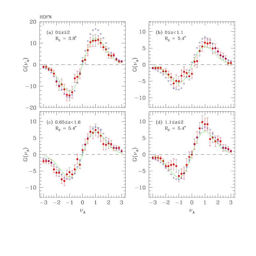
Figure 3: The genus curves (filled dotts) of the galaxy distributions of the HDF North subsamples. The solid lines are the Gaussian genus curves best fit to the observed data. The open circles are the average genus curve of 100 Poisson distributions with the same number of points as the number of galaxies in each HDF subsample.

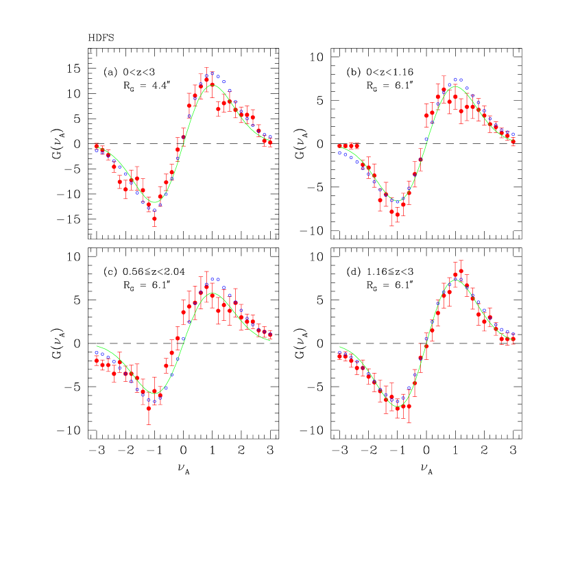
Figure 4: Same as Fig. 3 but for the HDF South subsamples.

Table 1: The HDF subsamples

Samples	$z$	$z_{\rm med}$	$N_{g}$(S/G-zone)	$R_{G}$
HDFN	$0.00\leq z\leq 2.00$	1.10	714/605	$3.8^{\prime\prime}$
HDFN-1	$0.00\leq z<1.10$	0.65	368/307	$5.4^{\prime\prime}$
HDFN-2	$0.65\leq z<1.60$	1.10	365/305	$5.4^{\prime\prime}$
HDFN-3	$1.10\leq z\leq 2.00$	1.60	346/298	$5.4^{\prime\prime}$
HDFS	$0.00\leq z\leq 3.00$	1.16	614/530	$4.4^{\prime\prime}$
HDFS-1	$0.00\leq z<1.16$	0.56	300/204	$6.1^{\prime\prime}$
HDFS-2	$0.65\leq z<2.04$	1.16	310/364	$6.1^{\prime\prime}$
HDFS-3	$1.16\leq z\leq 3.00$	2.04	314/266	$6.1^{\prime\prime}$

Table 2: Genus-related statistics for the HDF subsamples

Samples	$A$	${\bar{A}}_{\rm Poisson}$	$\Delta\nu-\Delta\nu_{\rm Poisson}$	$\Delta g-\Delta g_{\rm Poisson}$
HDFN	$20.3\pm 2.3$	26.5	$-0.01\pm 0.08$	$-0.22\pm 0.17$
HDFN-1	$9.1\pm 1.5$	13.2	$+0.30\pm 0.10$	$+0.21\pm 0.21$
HDFN-2	$11.4\pm 1.5$	13.2	$-0.01\pm 0.11$	$-0.14\pm 0.19$
HDFN-3	$11.5\pm 2.7$	13.2	$+0.03\pm 0.07$	$+0.35\pm 0.13$
HDFS	$19.2\pm 1.9$	22.4	$-0.15\pm 0.07$	$-0.12\pm 0.14$
HDFS-1	$10.6\pm 0.9$	11.7	$-0.17\pm 0.10$	$-0.31\pm 0.16$
HDFS-2	$7.2\pm 1.2$	11.7	$-0.25\pm 0.15$	$-0.24\pm 0.28$
HDFS-3	$12.0\pm 1.1$	11.7	$+0.03\pm 0.11$	$-0.19\pm 0.16$

References

- Clements & Couch (1996) Clements, D. L., & Couch, W. J. 1996, MNRAS, 280, L43
- (2) Coles, P. 1988, MNRAS, 234, 509
- (3) Coles, P., & Barrow, J. D. 1987, MNRAS, 228, 407
- (4) Coles, P., & Plionis, M. 1991, MNRAS, 250, 75
- (5) Colley, W. N. 1997, ApJ, 489, 471
- (6) Colley, W. N., Gott, J. R., & Park, C. 1996, MNRAS, 281, L82
- (7) Fernández-Soto, A. 2000, private communication
- (8) Fernández-Soto, A., Lanzetta, K. M., & Yahil, A. 1999, ApJ, 513, 34
- (9) Gott, J. R., Melott, A. L., & Dickinson, M. 1986, ApJ, 306, 341
- (10) Gott, J. R., Park, C., Juszkiewicz, R., Bies, W. E., Bennett, D., P., Bouchet, F. R., & Stebbins, A. 1990, ApJ, 352, 1
- (11) Gott, J. R., Mao, S., Park, C., & Lahav, O. 1992, ApJ, 385, 26
- (12) Gott, J. R., & Turner, E. L. 1979, ApJ, 232, L79
- (13) Gott, J. R., Weinberg, D., & Melott, A. L. 1987, ApJ, 319, 1
- (14) Hamilton, A. J. S., Gott, J. R., & Weinberg, D. 1986, ApJ, 309, 1
- (15) Kogut, A., Banday, A. J., Bennett, C. L., Gorski, K. M., Hinshaw, G., Smoot, G. F., & Wright, E. L. 1996, ApJ, 464, L29
- (16) Lanzetta, K. M., Chen, H.-W., Fernández-Soto, Pascarelle, S., Yahata, N., & Yahil, A. 1999, astro-ph/9910554
- Madau et al. (1996) Madau, P., Ferguson, H. C., Dickinson, M., Giavalisco, M., Steidel, C. C., & Fruchter, A. 1996, MNRAS, 283, 1388
- (18) Melott, A. L., Cohen, A. P., Hamilton, A. J. S., Gott, J. R., & Weinberg, D. H. 1989, ApJ, 345, 618
- Oke (1974) Oke, J. B., 1974, ApJS, 27, 21
- (20) Park, C., Colley, W. N., Gott, J. R., Ratra, B., Spergel, D. N., & Sugiyama, N. 1998, ApJ, 506, 473
- (21) Park, C., & Kim, J. 1998, ApJ, 501, 23
- (22) Park, C., Gott, J. R., Melott, A. L., & Karachentsev, I. D. 1992, ApJ, 387, 1
- (23) Smoot, G. F., Tenorio, L., Banday, A. J., Kogut, A., Wright, E. L., Hinshaw, G., & Bennett, C. L. 1994, ApJ, 437, 1
- Steidel et al. (1996) Steidel, C. C., Giavalisco, M., Dickinson, M., & Adelberger, K. L. 1996, AJ, 112, 352
- Williams et al. (1996) Williams, R. E. et al. 1996, AJ, 95, 107
- (26) Yahata, N., Lanzetta, K. M., Chen, H., Fernández-Soto, A., Pascarelle, S. M., Yahil, A., & Puetter, R. C. 2000, ApJ, 538,493
- (27) Weinberg, D. M. 1988, PASP, 100, 1373