Orbit Fitting and Uncertainties for Kuiper Belt Objects

Abstract

We present a procedure for determination of positions and orbital elements, and associated uncertainties, of outer Solar System planets. The orbit-fitting procedure is greatly streamlined compared to traditional methods because acceleration can be treated as a perturbation to the inertial motion of the body. These techniques are immediately applicable to Kuiper Belt Objects, for which recovery observations are costly. Our methods produce positional estimates and uncertainty ellipses even in the face of the substantial degeneracies of short-arc orbit fits; the sole a priori assumption is that the orbit should be bound or nearly so. We use these orbit-fitting techniques to derive a strategy for determining Kuiper Belt orbits with a minimal number of observations.

1 Introduction

The discovery of the Kuiper Belt (Jewitt and Luu, 1993) created a new vista upon the formation and early evolution of the Solar System. Study of these objects’ basic physical properties of course requires sufficiently well-determined orbital parameters to deduce a future position and the distance to the object. The orbital parameters are themselves of great interest, with the phase space of orbits threaded by an intricate web of resonant and long-lived chaotic zones (Malhotra, 1996). For both the practical goal of object retrieval and the higher goal of understanding the dynamical structure of the population, it is essential to not only have accurate orbits but also to quantify the uncertainty in the orbit.

There are centuries-old methods for determination of orbital parameters from observed positions. Present-day desktop computers execute these solutions trivially, and a linearized propagation of the positional uncertainties into the orbital elements is straightforward as well (Muinonen and Bowell, 1993). Workstations are even fast enough to bound the uncertainty region with a brute-force sampling of the 6-dimensional orbit space in many cases. Why then should we bother developing another orbit-fitting technique? KBOs pose a particular challenge because the objects are faint, so recovery observations are quite costly, requiring substantial investment of 2–4-meter telescope time for all but the brightest known objects. As a consequence, most known objects have been observed only a few times, leading to substantial degeneracies in the orbit fits. We need to know the error ellipse (in sky position and in orbital parameter space) even in the face of these degeneracies. In the best case a brute-force method will work on underdetermined orbits but leave us ignorant of the nature of the degeneracy. In the worst case the degeneracies will lead to long or effectively infinite computation times.

The Minor Planet Center (MPC) (http://cfa-www.harvard.edu/iau/mpc.html) provides orbital elements and predicted ephemerides for new objects. The approach of the MPC to short-arc objects is to select the simplest “sensible” orbit that fits the data—e.g. a circular orbit, if it fits the data and does not imply a close approach to Neptune; a 3:2 resonant orbit with Neptune if the circular orbit would imply a close approach; or, if the circular orbit is a poor fit, a “Väisälä” orbit, with the object near perihelion (Marsden, 1985, 1991), if this does not imply a close encounter. The MPC orbits in effect remove the degeneracies by assuming that the orbit is most likely to resemble those of known objects, and consequently predict positions that in most cases are quite close to the actual recovery positions. There are a few difficulties with this approach, however: first, focussing recovery efforts on the positions predicted by these favored orbits will inevitably bias the recovered population toward such orbits. This makes it difficult to quantify the portion of the population which may be in unusual orbits as they are preferentially lost. Second, uncertainties on positions and orbital elements are not currently available from the Minor Planet Center. Positional uncertainties are essential for proper planning and evaluation of recovery observations. Uncertainties on orbital elements are important for analyses of the dynamical characteristics of the population. For example, there was speculation that the 2:1 resonance with Neptune was empty or underpopulated, but 1997 SZ₁₀ and 1996 TR₆₆ were reclassified from 3:2 resonators to 2:1 resonators after further observations. Finally, it is sometimes necessary to calculate orbits “on the fly” during an observing run, and the MPC should not be expected to provide instantaneous analyses.

2 Methods

2.1 Motivation

Our approach to orbit-fitting for KBOs is motivated and guided by the following differences from the historically more common application to the asteroid population:

• Recovery observations are very expensive, as noted. This leads us to investigate, in §4, the minimal number of observations required to reach a given accuracy in orbital elements. The prediction of future positions should be a stable procedure even in the presence of nearly-degenerate orbital elements. This will require that we fully understand the nature of the degeneracies from short arcs. We would like to find a parameterization of the orbits in which the degeneracies are confined to as few parameters as possible.

• The release of the USNO-A2.0 astrometric catalog now makes it possible to measure astrometric positions to 0$\farcs$2 accuracy over the full sky (Deutsch, 1999) in a typical CCD image, and to produce reasonable estimates of the uncertainties on each position measurement. Uncertainty estimation can therefore proceed by the straightforward propagation of measurement errors. Space telescopes and adaptive-optics ground-based telescopes will commonly produce relative positions to 0$\farcs$01 accuracy in the near future. Very accurate positions should in principle produce accurate orbits even over relatively short arcs.

• KBOs are at distances $d\gtrsim 30$ AU so their apparent motions are dominated by reflex motion. The observed arcs are a small fraction of the orbital period $P$ even after a decade. Apparent motion patterns are thus very simple and unambiguous in comparison, say, to Near-Earth Objects.

• If we parameterize the distance to the object by $\gamma=(1{\rm\,AU})/d\lesssim 0.03$, the acceleration of the KBO is $\gamma^{2}\lesssim 10^{-3}$ times smaller than Earth’s acceleration, and the component transverse to the line of sight is $\gamma^{3}\approx 10^{-4.5}$ times Earth’s. The KBO motion is nearly inertial, and gravitational acceleration can be treated as a perturbation. Instead of parameterizing orbits by the usual element vector ${\bf a}=\{a,e,i,\Omega,\omega,T_{p}\}$, an orbit is more stably specified by some Cartesian phase space vector ${\bf P}=\{x_{0},y_{0},z_{0},\dot{x}_{0},\dot{y}_{0},\dot{z}_{0}\}$ at the time of initial observation.

• The annual parallax is limited to $2\gamma\approx 3\arcdeg$, and the total object motion is only $\approx 10\arcdeg$ over a decade. We will therefore express sky positions as coordinates $(\theta_{x},\theta_{y})$ in a tangent-plane projection of the celestial sphere about an appropriate reference point, e.g. the first observed location. Furthermore, the line of sight to the object changes by only a few degrees, and we will find it convenient to align our Cartesian coordinates with the $z$ axis along the initial line of sight.

• Daily parallax is $\leq 8\times 10^{-5}\gamma\lesssim 0\farcs 5$. For most ground-based observations this will be too small to yield useful information.

2.2 Exact Equations

The input data are the observed right ascension and declination $(\alpha_{i},\delta_{i})$ of the target at times $t_{i}$. We will assume that all positions have been measured in the J2000 celestial reference frame via astrometry tied to background stars in the USNO-A2 catalog. Measuring relative to the background stars exactly cancels the effects of stellar aberration, and reduces the maximal error from gravitational deflection of starlight to the milli-arcsecond level, so we can treat the problem with Euclidean geometry. We transform the observed coordinates to a tangent-plane projection $(\theta_{x},\theta_{y})$ about a reference location $(\alpha_{0},\delta_{0})$. The $\theta_{x}$ axis is taken in the Eastward direction of the J2000 ecliptic coordinate system, and $\theta_{y}$ points toward J2000 ecliptic North. Formulae for the conversion from $(\alpha,\delta)$ to $(\theta_{x},\theta_{y})$ are straightforward and summarized in Appendix A. Figure 1 illustrates the relation of our coordinate systems to the ecliptic.

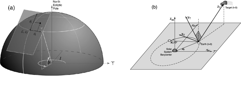
Figure 1: Panel (a) illustrates the relation of our angular coordinate system to ecliptic coordinates. Our coordinates are a tangent-plane projection of the sky about the initial line of sight, $(\ell_{0},b_{0})$. Panel (b) illustrates the spatial coordinate system ${\bf x}_{T}$ we adopt in relation to the ecliptic spatial system ${\bf x}_{\rm ec}$. Our system has origin at the observer location on Earth’s surface for $t=0$ and the $\hat{z}$ axis along the initial line of sight to the target. The vectors ${\bf x}_{E}$ and ${\bf x}_{B}$ toward the observer and solar system barycenter are illustrated as well. Both spatial and angular $\hat{x}$ and $\hat{y}$ axes are aligned to local ecliptic East and North, respectively.

We will generally take this projection axis to be the first observed position, and will take the first observation to be at time $t_{0}=0$. We will assume that $\theta_{x}$ and $\theta_{y}$ have equal and uncorrelated measurement uncertainties $\sigma_{i}$ (generalization to non-circular error regions is straightforward).

We define our inertial Cartesian coordinate system by placing the origin at (or near) the location of the observer at the initial epoch $t=0$. The $z$ axis is directed toward the reference direction $(\alpha_{0},\delta_{0})$ of the tangent-plane projection, i.e. along the initial line of sight. The $y$ axis is in the plane containing the $z$ axis and the J2000 North ecliptic pole, i.e. parallel to the $\theta_{y}$ axis of the tangent plane. The $x$ axis then lies in the ecliptic plane and points along $\theta_{x}$ to ecliptic East. Unless otherwise specified, we will take the units of distance and time to be AU and Julian year, respectively. The coordinate systems are illustrated in Figure 1.

If ${\bf x}(t)$ represents the position of the target at time $t$ and ${\bf x}_{E}(t)$ is the position of the observer on Earth, then the observed sky position at time $t$ is

$$\begin{array}[]{ccc}\theta_{x}(t)&=&{{x(t-\Delta t)-x_{E}(t)}\over{z(t-\Delta t)-z_{E}(t)}}\\ \theta_{y}(t)&=&{{y(t-\Delta t)-y_{E}(t)}\over{z(t-\Delta t)-z_{E}(t)}}\end{array}$$ (1)

where $\Delta t$ is the light-travel time $|{\bf x}(t-\Delta t)-{\bf x}_{E}(t)|/c$. The definition of $\Delta t$ is recursive but in practice is easily solved for iteratively because of the lack of ambiguity in KBO orbit solutions.

We wish our uncertainties to be limited by the errors in the astrometric catalog, so our requirement is to model the target position to $<0\farcs 1$ accuracy over $\approx 10$-year time spans. For target distance $\gtrsim 30$ AU, the object and observer positions must be correct to $\approx 2000$ km. The Earth’s position relative to the Sun and Solar System barycenter (SSB) is available from the JPL DE405 Ephemeris (Standish et al., 1995) to an accuracy many orders of magnitude better than we require. A simplistic model of the Earth as an oblate spheroid in constant rotation gives the observatory position to accuracy well within our tolerance, so we may consider ${\bf x}_{E}$ to be known exactly. The interpolated JPL ephemeris and topocentric correction are rapidly calculable.

2.2.1 Orbit Approximations

We write the target orbit as

$${\bf x}(t)={\bf x}_{0}+{\bf\dot{x}}_{0}t+{\bf g}(t),$$ (2)

where ${\bf g}$ is the gravitational perturbation satisfying

$${\bf g}(t=0) = \dot{\bf g}(t=0)=0,$$ (3)

$$\ddot{\bf g}(t) = \sum_{j}{-{GM_{j}[{\bf x}(t)-{\bf x}_{j}(t)]}\over{|{\bf x}(t)-{\bf x}_{j}(t)|^{3}}},$$ (4)

where the sum runs over the other bodies in the Solar System. We include forces from the Sun and the giant planets, obtaining their positions from the DE405 ephemeris. For objects beyond 30 AU, one could approximate the total gravitational field of the Solar System as a monopole originating the Solar System barycenter, with errors of only $\sim 10^{-4}$ AU over 10 years (barring Neptune encounters), yielding positions accurate to $<1\arcsec$. The computational expense of the full N-body form Eq. (4) is insignificant, however, as the time steps in the orbit integration can be quite long (20 days or more) without significant loss of accuracy over a decade.

The combination of Eqs. (1), (2), and (4) define our model for the position $(\theta_{x},\theta_{y})$ as a function of time and the initial state vector ${\bf P}$. A comparison of our positions for Pluto, Neptune, and 1992 QB1 to those generated by the JPL ephemeris indicate residual differences of $<0\farcs 05$ for a 10-year integration.

2.3 Approximate Formulae & Degeneracies

We can understand the nature of the short-arc degeneracies by expanding Eq. (1) in powers of time $t$ and distance parameter $\gamma$. The formulae are simpler if we redefine our phase space basis in terms of the vector $\mbox{{\boldmath$\alpha$}}=\{\alpha,\beta,\gamma,\dot{\alpha},\dot{\beta},\dot{\gamma}\}$, where

$$\begin{array}[]{lll}\alpha\equiv{x_{0}}/{z_{0}}&\beta\equiv{y_{0}}/{z_{0}}&\gamma\equiv 1/{z_{0}}\\ \dot{\alpha}\equiv{\dot{x}_{0}}/{z_{0}}&\dot{\beta}\equiv{\dot{y}_{0}}/{z_{0}}&\dot{\gamma}\equiv{\dot{z}_{0}}/{z_{0}}.\end{array}$$ (5)

Please note that $\dot{\alpha}$, $\dot{\beta}$, and $\dot{\gamma}$ quantify the motion along our three axes but are not the time derivatives of $\alpha$, $\beta$, and $\gamma$. We have chosen our coordinate system so that $\alpha,\beta\approx 0$, and we expect $\dot{\alpha},\dot{\beta},\dot{\gamma}\sim 2\pi\gamma^{3/2}$ for bound orbits. If the orbit is nearly circular, the line-of-sight velocity is down another factor of $\gamma$ so that $\dot{\gamma}\sim 2\pi\gamma^{5/2}$. The $x$ component of the apparent motion is now

$$\theta_{x} = {{\alpha+\dot{\alpha}t+\gamma g_{x}(t)-\gamma x_{E}(t)}\over{1+\dot{\gamma}t+\gamma g_{z}(t)-\gamma z_{E}(t)}}$$ (6)

$$\approx \alpha+(\dot{\alpha}-\gamma\dot{x}_{E})t$$

$$+\gamma(\ddot{g}_{x}-\ddot{x}_{E})t^{2}/2-(\dot{\gamma}-\gamma\dot{z}_{E})(\dot{\alpha}-\gamma\dot{x}_{E})t^{2}$$

$$+O(t^{3}).$$

In the second line we have made the approximation that $t\ll 1$ year. The equation for $\theta_{y}$ is analogous. We see that the solution for the orbital parameters $\alpha$ has three regimes:

2.3.1 Slope Regime

For arcs spanning consecutive nights, we can only determine the instantaneous positions $\alpha$ and $\beta$, plus the slopes

$$\dot{\theta}_{x} = (\dot{\alpha}-\gamma\dot{x}_{E})\approx\dot{\alpha}-\gamma(2\pi\cos\phi_{0})$$ (8)

$$\dot{\theta}_{y} = (\dot{\beta}-\gamma\dot{y}_{E})\approx\dot{\beta}$$ (9)

The approximations assume that we are observing near the ecliptic plane, and that the Earth’s orbit is circular with phase $\phi_{0}$ at time $t=0$ relative to the Sun-target vector. In this situation the line-of-sight motion $\dot{\gamma}$ is completely unconstrained, and there is a total degeneracy between the distance $\gamma$ and the ecliptic motion $\dot{\alpha}$. For a circular orbit, $|\dot{\alpha}|\approx(\sqrt{\gamma}/\cos\phi_{0})(\gamma\dot{x}_{E})$, and for any bound orbit $|\dot{\alpha}|<(\sqrt{2\gamma}/\cos\phi_{0})(\gamma\dot{x}_{E})$. The usual observational strategy, therefore, is to observe near opposition ($\phi_{0}=0$) to minimize the proper-motion term $\dot{\alpha}$ relative to the parallax term $\gamma\dot{x}_{E}$, giving an estimate of $\gamma$ to fractional accuracy of $\sqrt{2\gamma}\approx 0.25$ or better. An ephemeris may be predicted under the assumption of a prograde circular orbit. Below we will describe a simple way to place an error ellipse on the position without assuming a circular orbit.

2.3.2 Acceleration Regime

As the arc length grows, the next bit of information gleaned is the apparent acceleration vector:

$$\ddot{\theta}_{x} = \gamma(\ddot{g}_{x}-\ddot{x}_{E})-2(\dot{\gamma}-\gamma\dot{z}_{E})(\dot{\alpha}-\gamma\dot{x}_{E})$$ (10)

$$\approx \gamma(\ddot{g}_{x}-4\pi^{2}\sin{\phi_{0}})+2\dot{\gamma}\ (2\pi\gamma\cos{\phi_{0}}).$$ (11)

The second line again assumes an ecliptic observation and a circular Earth orbit, and keeps leading-order terms only. We see first that the effect of $\dot{\gamma}$ on the acceleration is a factor $\gamma/2\pi<0.005$ smaller than the $\gamma\ddot{x}_{E}$ term. In this regime, therefore, $\dot{\gamma}$ is still indeterminate. The target’s transverse acceleration $\ddot{g}_{x}$ is smaller by a factor $\gamma^{3}$ than the Earth’s acceleration and can also be ignored at this point. The apparent acceleration is then

$$\ddot{\theta}_{x} \approx -\gamma(4\pi^{2}\sin{\phi_{0}})$$ (12)

$$\ddot{\theta}_{y} \approx 0$$

We see that the apparent acceleration is a robust and simple way to constrain $\gamma$, the distance to the target. This method fails however, for observations at opposition ($\phi_{0}=0$), where the reflex acceleration vanishes.

What time span is needed to measure the acceleration to a useful accuracy? Let us presume that the object is initially detected in a pair of observations separated by 24 hours, then recovered in a single observation some time $T$ later, and that each observation has astrometric uncertainty $\sigma$. Using Eq. (12) to determine $\gamma$, the fractional error in the distance to the target is then roughly

$${\sigma_{d}\over d} = {\sigma_{\gamma}\over\gamma}\approx{\sigma\over{\sqrt{2}\pi^{2}\gamma\sin{\phi_{0}}(24\,{\rm h})T}}$$

$$= 7.5\%\left({\sigma\over 0\farcs 2}\right)\left({1{\,\rm week}\over T}\right)\left({\sin 45\arcdeg\over\sin\phi_{0}}\right)\left({d\over 40{\,\rm AU}}\right)$$

The distance to most KBOs can be determined from the apparent acceleration with only 1 week’s arc, as long as the observations are not near opposition. For a main belt asteroid, the apparent acceleration is an order of magnitude larger and is easily detected in a 24-hour span. This means it is easy to distinguish main belt asteroids from KBOs away from opposition, even near the main-belt turnaround points.

A typical (non-opposition) 1-week arc thus gives a useful estimate of 5 of the 6 phase-space parameters of the orbit, with the line-of-sight motion being completely indeterminate. In this basis the degeneracy is confined to a single parameter, whereas the degeneracy is shared between most of the traditional orbital elements. In particular neither $a$ nor $e$ is at all well constrained at this point.

It is interesting to note that the orbital angular momentum is sensibly constrained in this regime, since the line-of-sight velocity is nearly radial to the Sun and contributes little to the angular momentum. The energy of the orbit, however, is

$$E=-GM_{\odot}\gamma(1-2\gamma\cos\beta_{0}+\gamma^{2})^{-1/2}+(\dot{\alpha}^{2}+\dot{\beta}^{2}+\dot{\gamma}^{2})/2\gamma^{2},$$ (14)

and is uncertain until $\dot{\gamma}$ can be constrained. Here $\beta_{0}$ is the solar elongation of the target at the initial epoch.

2.3.3 Fully Constrained Regime

The line-of-sight velocity can be constrained as the Earth moves around its orbit to give us a new point of view. From Eq. (6), the leading $\dot{\gamma}$ term in the sky position is $\dot{\gamma}t\gamma x_{E}(t)\lesssim\dot{\gamma}\gamma t$. We know that $\dot{\gamma}^{2}<2GM_{\odot}\gamma^{3}$ from the simple constraint that the object be bound. A useful constraint on $\dot{\gamma}$ is obtained only after sufficient time that a $\dot{\gamma}$ value below the binding limit would produce a measured displacement that is distinguishable from terms in the other 5 parameters. This can occur on a timescale of months for high-quality observations. The uncertainty in $\dot{\gamma}$ (or $\dot{z}$) dominates the phase space uncertainties for essentially all lengths of arc, though it does not always dominate the ephemeris uncertainties.

2.4 Fitting Procedures

With 3 or more observations spanning several months or more, we will be in the fully-constrained regime. At this point the constraint of the orbital parameter vector $\alpha$ from the measured positions $\mbox{{\boldmath$\theta$}}_{i}$ becomes a straightforward non-linear minimization problem. The formalism for Bayesian orbit fitting is discussed in detail by Muinonen and Bowell (1993). We will assume Gaussian measurement errors, in which case the most likely parameter vector $\hat{\alpha}$ is the least-squares value, minimizing

$$\chi^{2}=\sum_{i}\left\{{[\theta_{x,i}-\theta_{x}(\mbox{{\boldmath$\hat{\alpha}$}},t_{i})]^{2}\over\sigma_{i}^{2}}+{[\theta_{y,i}-\theta_{y}(\mbox{{\boldmath$\hat{\alpha}$}},t_{i})]^{2}\over\sigma_{i}^{2}}\right\}.$$ (15)

The model $\theta_{x}(\mbox{{\boldmath$\hat{\alpha}$}},t_{i})$ for the predicted position is embodied by Eqs. (5), (1), (2), and (4). The minimization of $\chi^{2}$ can use standard algorithms. We have implemented a slight modification of the Levenberg-Marquardt method from Press et al. (1988). For efficient location of the minimum, we require a good starting point for the non-linear search, and estimates of the derivative matrix $d{\bf\theta}/d\mbox{{\boldmath$\alpha$}}$.

The determination of the derivatives is again greatly simplified for distant objects. The gravitational acceleration is, over a $\lesssim 10$-year period, a small perturbation to the inertial motion, barring close encounters. The inertial motion will be $\sim 2\pi\sqrt{\gamma}t$ and the acceleration term will integrate to $\approx 4\pi^{2}\gamma^{2}t^{2}/2$. Furthermore the acceleration is toward the barycenter, so the transverse component is down by another factor of $\gamma$. The angular displacement due to gravity is only a few arcseconds per year, $\gtrsim 300$ times smaller than the inertial motion and reflex motion. It is clear that in calculating the derivative matrix $\partial{\bf x}/\partial\mbox{{\boldmath$\alpha$}}$ from Eq. (2) that we can ignore the gravitational term. All of the derivatives are thus quite trivial and there is no need to integrate the derivatives of the orbit.

Selection of a sensible starting point for the minimization is also simple for distant objects. We produce a version of the equations of motion which ignores gravity, is linearized, and also ignores the $\dot{\gamma}$ term:

$$\theta_{x}\approx\alpha+\dot{\alpha}t-\gamma x_{E}(t),$$ (16)

$$\theta_{y}\approx\beta+\dot{\beta}t-\gamma y_{E}(t),$$

These equations are linear in the parameter vector $\alpha$ and hence have a closed-form minimization requiring only the inversion of a $5\times 5$ matrix (Press et al., 1988). These very simple equations are actually good to a few arcseconds for the first year of observation, and in any case provide (with $\dot{\gamma}=0$) a good starting point for the non-linear minimization.

Using the analytic derivatives, the Levenberg-Marquardt algorithm also calculates the covariance matrix ${\bf\Sigma}_{\alpha}$ of the fitted parameters. Since the model $\mbox{{\boldmath$\theta$}}(\mbox{{\boldmath$\alpha$}},t)$ is dominated by terms linear in the parameters, the linearized approximation

$$\Delta\chi^{2}=(\mbox{{\boldmath$\alpha$}}-\mbox{{\boldmath$\hat{\alpha}$}})^{T}{\bf\Sigma}_{\alpha}(\mbox{{\boldmath$\alpha$}}-\mbox{{\boldmath$\hat{\alpha}$}})$$ (17)

will be accurate even for poorly constrained orbits. This would not have been the case had we chosen the orbital-element vector ${\bf a}$ as the parameter set.

2.5 Position and Orbital Element Estimation

Once the best-fit $\hat{\alpha}$ vector and its covariance matrix are determined from the fit, determination of orbital elements and future positions is also simple. The predicted position at any time $t$ is $\mbox{{\boldmath$\theta$}}(\mbox{{\boldmath$\hat{\alpha}$}},t)$. The uncertainty ellipse for the position is specified by the covariance matrix

$${\bf\Sigma}_{\theta}=\left({d\mbox{{\boldmath$\theta$}}(\mbox{{\boldmath$\alpha$}},t)\over d\mbox{{\boldmath$\alpha$}}}\right)^{T}{\bf\Sigma}_{\alpha}\left({d\mbox{{\boldmath$\theta$}}(\mbox{{\boldmath$\alpha$}},t)\over d\mbox{{\boldmath$\alpha$}}}\right).$$ (18)

The derivatives, as above, are rapidly calculated by ignoring gravity. Again the position is nearly linear in our chosen orbital basis, so this linearized transformation will be accurate even in the case of large uncertainties in the parameters.

The best-fit orbital element vector ${\bf\hat{a}}$ is determined from the best-fit phase-space parameter set $\hat{\alpha}$ via the usual equations, which are reviewed in Appendix B. The determination of an uncertainty ellipsoid in orbital-element space requires mapping of the covariance matrix with the derivatives $d{\bf a}/d\mbox{{\boldmath$\alpha$}}$. Some of these derivatives are quite complicated analytic expressions, but can still be coded and rapidly evaluated. The map from $\alpha$ to ${\bf a}$ is non-linear, and in some cases degenerate, so the linearized covariance matrix is formally correct only when the uncertainties in the elements become small. We do, however, obtain a useful estimate of the element uncertainties even for less exact determinations.

2.5.1 Fitting Singly Degenerate Orbits

If the arc is too short, the minimization of $\chi^{2}$ will proceed but the best-fit parameters may be non-physical. The degeneracy in the “acceleration regime” will be manifested as one or more large elements of the covariance matrix. In particular, several-week orbits will have large values of $\Sigma_{\dot{\gamma}\dot{\gamma}}$. We recognize these orbits as unrealistic because they may be unbound. The assumption of a bound orbit limits $\dot{\gamma}$ to (cf. Eq. [14])

$$\dot{\gamma}^{2}\leq\dot{\gamma}^{2}_{\rm bind}=GM_{\odot}\gamma^{3}(1+\gamma^{2}-2\gamma\cos\beta_{0})^{-1/2}-\dot{\alpha}^{2}-\dot{\beta}^{2}.$$ (19)

A conservative approach to assigning uncertainties in this case is to assume that $\dot{\gamma}$ has a uniform a priori probability in the interval $[-\dot{\gamma}_{\rm bind},+\dot{\gamma}_{\rm bind}]$. If, however, we assign a Gaussian prior distribution to $\dot{\gamma}$, we can preserve our least-squares approach to the fitting problem. We therefore fit by assuming that $\dot{\gamma}=0$ with an RMS uncertainty of $\sigma_{\rm bind}=\dot{\gamma}_{\rm bind}/\sqrt{3}$. This value of $\sigma_{\rm bind}$ has the same variance as the uniform distribution, and the entire $\pm\dot{\gamma}_{\rm bind}$ range (plus some marginally unbound orbits) is contained within the $2\sigma$ contour, so we will obtain a realistic assessment of the uncertainties.

Our procedure for handling the $\dot{\gamma}$ degeneracy is thus:

1. Fit the orbit with all six parameters free to vary.

2. If the unconstrained fit yields $\Sigma_{\dot{\gamma}\dot{\gamma}}<\sigma^{2}_{\rm bind}$, then $\dot{\gamma}$ is well constrained by the observations and we are done. Otherwise $\dot{\gamma}$ is essentially decoupled from the observations, so we proceed using the binding constraint instead.

3. Re-fit the observations but set $\dot{\gamma}=0$ and derive values and a covariance matrix for the remaining 5 parameters. Note that this best-fit orbit is very similar to the Väisälä orbit, as a line-of-sight velocity near zero implies an orbit near its perihelion or aphelion.

4. Augment the covariance matrix by assigning $\Sigma_{\dot{\gamma}\dot{\gamma}}=\sigma^{2}_{\rm bind}$, placing zeros in the remaining off-diagonal elements.

The best-fit parameters $\hat{\alpha}$ and covariance ${\bf\Sigma_{\alpha}}$ may then be used to predict positions and orbital elements as in the non-degenerate case. The $2\sigma$ error ellipses will encompass $>95\%$ of all bound orbits that are consistent with the data, and not be restricted to circular or perihelic orbits. If we have some preconceptions about the maximal ellipticity of the orbits, this may be incorporated into the position predictions by placing a tighter a priori constraint on $\dot{\gamma}$.

2.5.2 Fitting Doubly Degenerate Orbits

With only a single or few nights’ data, or if there are only 2 observations, we are in the “slope regime.” The above technique will fail due the additional degeneracy between $\dot{\alpha}$ and $\gamma$ (and $\dot{\beta}$ for observations out of the ecliptic plane). This will manifest itself in the covariance matrix obtained in Step 3 above, the 5-parameter fit to the orbit. The uncertainties $\Sigma_{\dot{\alpha}\dot{\alpha}}$ and/or $\Sigma_{\dot{\beta}\dot{\beta}}$ will be large.

In this case we again introduce the binding constraint to limit the extent of the degeneracy. We express the transverse kinetic energy in terms of a parameter $f_{b}$:

$$\dot{\alpha}^{2}+\dot{\beta}^{2}=(1+f_{b})GM_{\odot}\gamma^{3}.$$ (20)

The binding constraint is then $-1<f_{b}<1$, with $f_{b}=0$ corresponding to a nearly circular orbit. We crudely implement this constraint by minimizing a new quantity

$$\tilde{\chi}^{2}=\chi^{2}+f_{b}^{2}/3.$$ (21)

(with $\chi^{2}$ from Eq. 15), which pushes the solution toward a circular orbit, while yielding a covariance matrix that reflects both the observational uncertainties and the possibility of non-circular orbits. More sophisticated constrained optimizations are possible but there is little point to seeking precise constraints on such a poorly determined orbit.

3 Implementation and Examples

3.1 C Code

All of the above algorithms have been implemented in a family of subroutines and drivers written in C. These include routines for: creation and access of binary versions of the DE405 ephemeris files (provided by David Hoffman); orbit integration; transformations among the various Cartesian and spherical coordinate systems; transformations between phase-space and orbital-element bases for orbits; reduction of positions to topocentric coordinates; and the fitting procedures described in the previous section. The code is portable and self-contained, and is available from the first author upon request.

The main program is fit_radec, which takes as input a list of astrometric observations, and executes the orbit-fitting, including proper handling of degeneracies. The output is a file specifying the best-fit $\alpha$ description of the orbit, and its full covariance matrix ${\bf\Sigma}_{\alpha}$.

A program abg_to_aei transforms the $\alpha$ parameters into traditional orbital elements. The covariance matrix is also transformed with a linear approximation.

The $\alpha$ information may be passed to the program predict, which generates predicted positions and their error ellipses for any specified observation date and site.

The entire process is extremely fast on the typical present-day desktop computer. A fit to 275 mock observations of Pluto over a 14-year arc takes about 1 second. The entire ensemble of observations of all $\approx 300$ KBOs reported to the MPC are fit in a few seconds.

3.2 Example and Verification

We have verified the performance of the algorithms and software by conducting mock observations of Pluto, Neptune, and several KBOs. Figure 2 shows the results of an ensemble of simulated observations of Pluto from 1995–1998. The true position of Pluto is obtained from the DE405 ephemeris; mock observations are created at specified dates by adding Gaussian deviations to the true positions. An orbit is then fit to the mock observations. This fitted orbit is used to estimate the osculating barycentric elements $a$ and $e$ for Pluto as well as the uncertainty ellipse in the $a$–$e$ plane. Alternatively we may use the orbit fit to estimate the $(\theta_{x},\theta_{y})$ sky position of Pluto at some future date and its projected error ellipse. We can then examine whether the estimated orbital elements or future position are consistent with the true ephemeris values. In all cases we find the mean $\chi^{2}$ value of the fit to the orbit to be as expected from the degrees of freedom in the fit.

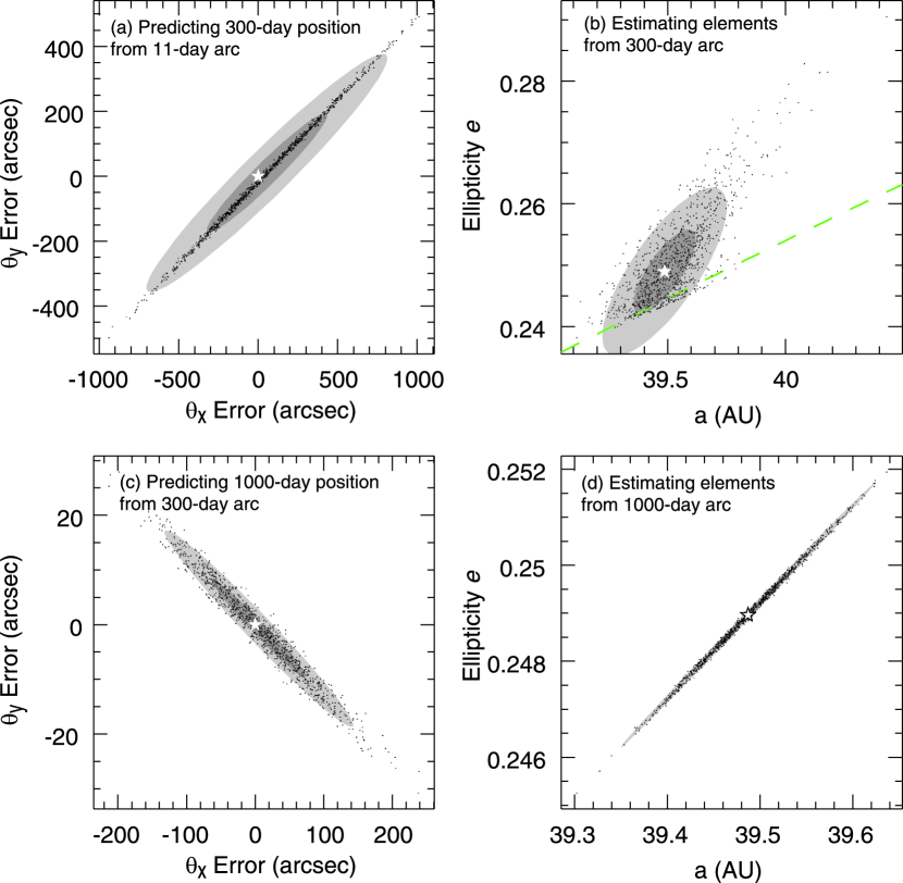
Figure 2: Demonstration of position/orbital element estimation using the methods described in the text. In the left panels (a) and (c), mock observations of Pluto are used to predict a future position on the sky. Each small symbol is the prediction from one mock arc; the star is the correct position, while the two shaded ellipses are the 1- and 2-sigma uncertainty regions produced by our methods. The panel (b) shows the orbital parameters $a$ and $e$ estimated from 5 observations over 300 days, along with the true position and estimated uncertainties. Panel (d) shows the elements estimated after an additional observation at 1000 days. The scatter of estimates matches the uncertainties except in case (b). Details of this failure are explained in the text.

The first panel in Figure 2 shows the results of using 4 observations over an 11-day arc (JD 2449927–2449938) to predict the location of Pluto $\approx 300$ days after the first observation. Each point on the plot is the prediction from one of 1000 realizations of the mock 11-day arc. The star shows the true location of Pluto at the 300-day time. The ellipses show the $1\sigma$ and $2\sigma$ contours of the estimated error on the position given the observational errors. The estimated uncertainty ellipse is quite consistent with the scatter in the mock predictions. There appear to be two flaws in our prediction: first, the mean of the predicted positions does not coincide with the true position; second, the minor axis of the uncertainty ellipse appears to be significantly larger than the scatter. Both of these phenomena are expected, however, because the 11-day arc is the “acceleration regime” and is degenerate in $\dot{\gamma}$. The fits therefore have assumed a value and uncertainty for $\dot{\gamma}$. The displacement of the simulations from the true value is due to our assumption that $\dot{\gamma}=0$ for each fit, which is not the true value. But the uncertainty ellipse includes a contribution from our ignorance of $\dot{\gamma}$, which makes the ellipse extend beyond the measured scatter, and in fact properly include the true position.

In the second panel we simulate an observation sequence consisting of the 11-day arc plus and additional observation at 300 days. We plot the estimated $a$ and $e$ values from 1000 mock observations of the 300-day arc. In this case the uncertainty ellipses give a roughly correct estimate of the size of the errors, but the scatter does not match the error ellipses in detail. This demonstrates a limitation of our method, which is that the propagation of the covariance matrix ${\bf\Sigma}_{\alpha}$ to the orbital elements is incorrect if the map between them is significantly nonlinear. This is the case here, as Pluto is very near perihelion at this time. The 300-day arc determines the distance to Pluto quite well, and hence the scatter plot is bounded by a lower limit to the perihelion $a(1-e)$.

The third panel shows the results of using the 300-day arc to predict the position after 1000 days, and the fourth panel shows the scatter in the $a$–$e$ plane of elements determined from 6 observations on a 1000-day arc. We can now usefully constrain all 6 parameters of the orbit, and the scatter about the true position and orbit are very accurately described by the estimated covariance matrices.

4 Optimal Strategies

An optimal schedule for recovery of KBOs would maximize some measure of the accuracy of the KBO orbit while minimizing the number of recovery observations required. A constraint on the observing schedule is that the positional uncertainty must not become larger than the field of view of the instrument, lest the recovery be missed and the object be lost. As an illustration of the utility of the methods described in this paper, we derive an optimal schedule of observations using a crude algorithm.

We take our measure of the quality of the orbit fit to be the uncertainty $\sigma_{a}=\sqrt{\Sigma_{aa}}$ in the semi-major axis of the orbit. This is not meant to be a universal metric for quality but rather a simple example. We place two constraints on the observing schedule: first, observations are not allowed when the solar elongation of the target is less than 90°. Second, we take the field of view of the recovery instrument to be $\approx 10\arcmin$; then the 1-sigma positional uncertainty must be $\leq 2\farcm 5$ if the full 2-sigma error ellipse is to be contained within the field of view for $>95\%$ chance of recovery. Note that many CCD mosaics currently on 2-meter and 4-meter class telescopes have fields of view that substantially exceed 10′.

A rigourous optimization for a set of $N$ observations would consider all possible sets of $N$ nights and choose the set which minimizes the final $\sigma_{a}$. We adopt a somewhat simpler “greedy” algorithm for optimization as follows: after observation $M$, we consider all nights for which observation $M+1$ would be possible, namely those satisfying the elongation ad positional uncertainty costraints. We next calculate the $\sigma_{a}$ which would result from an observation on each possible night; the $M+1$ observation is then scheduled for the night which would result in minimal $\sigma_{a}$.

Figure 3 illustrates the observation schedule derived for hypothetical discovery of Pluto in the year 1995. We assume that the object is discovered on a pair of nights roughly 45 days before opposition, then confirmed on another pair of nights 10 days later. We also presume that each observation has an error of $\sigma=0\farcs 2$. As seen in the Figure, the object must be observed once again in the discovery season as its uncertainty is too high to be recovered when it emerges from behind the Sun the following year. The object is now sufficiently well characterized to be found for nearly 3 years. When is the best time during this window to observe again? Interestingly the accuracy on $a$ improves only weakly the longer we wait for our next observation. The “greedy” strategy suggests we wait 3 years, when the positional uncertainty approaches 2$\farcm$5. So after the initial 4 discovery/confirmation images and only 2 recoveries, $\sigma_{a}\approx 0.03$ AU, and the orbit is known well enough to permit recovery for the next decade.

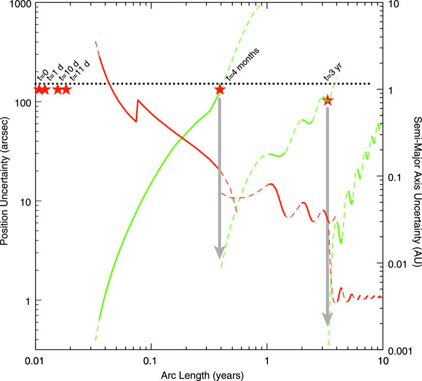
Figure 3: The observation optimization routine described in the text is applied here to Pluto. We assume an initial set of four observations over a 10 days, about 6 weeks before opposition. We then ask when further observations are best scheduled. The upward-sloping lines depict the uncertainty in position of the object given the 10-day arc; another observation must be done while the uncertainty is below 150″ (the dotted line) in order to assure successful recovery in a 10′ FOV. The curved is dashed when the target is too close to the Sun to observe, solid otherwise. The downward-sloping lines show the uncertainty in semi-major axis $a$ that would be obtained from a further observation at the given time. Additional observations (stars) are scheduled at the time during the recovery window when the measurement will most reduce the uncertainty on $a$. Each new observation then starts a new pair of curves for $a$ and position uncertainty. A new observation is needed at 4 months (before the target disappears behind the Sun), after which the uncertainty on $a$ is only weakly dependent upon the timing of observations. Another observation is needed within 3 years else the target becomes lost.

A counterintuitive result is that the timing of further observations has little effect upon the accuracy of $a$—only increased number and/or accuracy of observations matters at this point. This is because the uncertainty in $a$ derives primarily from the uncertainty in $\gamma$, i.e. the distance to the target. The leading observable consequence of $\gamma$ is the parallax $\gamma x_{E}(t)$, which does not grow with time beyond 1 year—hence the very weak improvement with longer arcs. Indeed we find that observing near the two quadratures of the second year yields a $\sigma_{a}$ that is as low as spacing these two observations over several years.

Another common observing scheme is to run discovery observations during two nights near opposition, then attempt confirmation one month later. For Pluto, the positional error is sufficiently small this second month to permit reliable confirmation. Henceforth the optimal strategy plays out just as the previous scenario: a further observation is required before quadrature to keep the object from being lost while behind the Sun, and the orbital quality depends primarily upon the number, not the arc length, of recoveries in later years.

If the astrometric accuracy of the initial 11-day arc can be improved to 0$\farcs$1, and the recovery tolerance raised to $\sigma_{a}\approx 10\arcmin$, then no further observations are required in the first year. The object is recoverable at the beginning of the second season, two observations (near the quadratures) in this second year reduce $\sigma_{a}$ to 0.0002 AU, and the position is good for a decade or more.

These results are of course dependent upon the orbit of the object and upon the nature of one’s metric for orbital quality. Our optimization method is, however, easily adapted to other metrics.

5 Summary

Orbit fits for KBOs and other distant objects are greatly simplified by the fact that the gravitational perturbation to the orbit is small compared both to the inertial motion and to the acceleration of the Earth. Gravity can be treated as a perturbation even for decades-long arcs, which simplifies the fitting process and the propagation of errors because there is no need to integrate the derivatives of the orbit. The orbit itself can be integrated quickly because large time steps can be taken. Distant objects move slowly across the sky, so we can also use the convenience of a tangent-plane projection of the celestial sphere. The dominance of reflex motion over proper motion means that KBO orbit solutions are unambiguous.

Exploiting these properties, we have created algorithms and software which quickly and accurately calculates orbital elements and ephemerides and their associated uncertainties for targets $\gtrsim 10$ AU from the Sun. In cases where the observed arc is short enough to leave the orbit degenerate, we can still calculate sensible positional errors because we have chosen an orbital basis in which the degeneracy is confined to one parameter, namely the line-of-sight velocity. For very short arcs in the “slope regime,” 2 additional parameters become degenerate. We are still able to place error ellipses on ephemerides which are conservative in the sense that they will include any bound orbit. Most short-arc objects will be recovered closer to the MPC predicted ephemeris than our error ellipses would suggest, because the philosophy of the MPC is to use the stronger a priori consideration that the orbits resemble those of the majority of the known populations.

Our routines should prove valuable for planning of recovery observations, as we have illustrated with some simple examples. Estimates of the uncertainty ellipsoids in orbital-element space will also be needed for study of the long-term dynamics of the known KBOs.

In the near future we expect that KBO positions will be measured to accuracies of a few milli-arcseconds with orbiting observatories—though such observations will be even more expensive than present-day KBO observations. It will then be possible to place strong constraints on KBO orbits even from very short (e.g. 24-hour) arcs. For example, the motion of an observatory in low-Earth orbit imparts a reflex motion on the KBO that is easily detected at this level, giving a measure of the distance to the target in less than an hour. The methods described herein will provide the means to plan and to analyze such observations.

Appendix A Coordinate Transformations

A.1 Angular Coordinates

We make use of three sets of coordinates on the celestial sphere: equatorial coordinates $(\alpha,\delta)$ in the ICRS reference frame, J2000; ecliptic latitude and longitude $(\ell,b)$, also taken in the epoch 2000 frame; and our projected coordinates $(\theta_{x},\theta_{y})$ measured in a tangent plane about some reference direction $(\alpha_{0},\delta_{0})$ or $(\ell_{0},b_{0})$. The transformation from equatorial to ecliptic coordinates is implemented as

$$\sin b = \cos\epsilon\sin\delta-\sin\epsilon\cos\delta\sin\alpha$$ (A1)

$$\tan\ell = {{\cos\epsilon\cos\delta\sin\alpha+\sin\epsilon\sin\delta}\over{\cos\delta\cos\alpha}},$$ (A2)

where $\epsilon=23\fdg 43928$ is the obliquity of the ecliptic at J2000 (Standish et al., 1995). The inverse transformation simply reverses the sign of $\epsilon$.

The map from ecliptic to tangent-plane coordinates about $(\ell_{0},b_{0})$ is

$$\theta_{x} = {{\cos b\sin{(\ell-\ell_{0})}}\over{\sin b_{0}\sin b-\cos b_{0}\cos b\cos{(\ell-\ell_{0})}}}$$ (A3)

$$\theta_{y} = {{\cos b_{0}\cos b-\sin b_{0}\sin b\cos{(\ell-\ell_{0})}}\over{\sin b_{0}\sin b+\cos b_{0}\cos b\cos{(\ell-\ell_{0})}}}.$$ (A4)

The inverse transformation is

$$\sin b = {{\sin b_{0}+\theta_{y}\cos b_{0}}\over\sqrt{1+\theta_{x}^{2}+\theta_{y}^{2}}}$$ (A5)

$$\sin{(\ell-\ell_{0})} = {{\theta_{x}/\cos b_{0}}\over\sqrt{1+\theta_{x}^{2}+\theta_{y}^{2}}}.$$ (A6)

Partial derivative matrices are straightforward for all transformations, and approximations for $\theta_{x},\theta_{y}\ll 1$ are particularly simple.

A.2 Spatial Coordinates

There are also three relevant spatial coordinate systems. The equatorial ${\bf x}_{\rm eq}$ has origin at the Solar System barycenter, with $x$ positive to the Vernal Equinox and $z$ positive to the North equatorial pole of J2000. The ecliptic system ${\bf x}_{\rm ec}$ also has origin at the barycenter, but $z$ is positive to the North ecliptic pole of J2000. Our “telescope-centric” coordinate system ${\bf x}_{T}$ has origin at the location of the observer at $t=0$, with $z$ positive along the line of sight to the target at $t=0$, the $y$ axis in the plane of $z$ and the North ecliptic pole—see Figure 1.

The transformation from equatorial to ecliptic coordinates is

$$\left[\begin{array}[]{c}x\\ y\\ z\\ \end{array}\right]_{\rm ec}=\left[\begin{array}[]{ccc}1&0&0\\ 0&\cos\epsilon&\sin\epsilon\\ 0&-\sin\epsilon&\cos\epsilon\\ \end{array}\right]\left[\begin{array}[]{c}x\\ y\\ z\\ \end{array}\right]_{\rm eq}$$ (A7)

The inverse transformation inverts the sign of $\epsilon$.

The transformation from ecliptic to telescope-centric coordinates is

$$\left[\begin{array}[]{c}x\\ y\\ z\\ \end{array}\right]_{T}=\left[\begin{array}[]{ccc}-\sin\ell_{0}&\cos\ell_{0}&0\\ -\cos\ell_{0}\sin b_{0}&-\sin\ell_{0}\sin b_{0}&\cos\ell_{0}\\ \cos\ell_{0}\cos b_{0}&\sin\ell_{0}\cos b_{0}&\sin\ell_{0}\\ \end{array}\right]\left[\begin{array}[]{c}x-x_{0}\\ y-y_{0}\\ z-z_{0}\\ \end{array}\right]_{\rm ec}.$$ (A8)

The ecliptic-coordinate location of the observer at time $t=0$ is given by the vector $\{x_{0},y_{0},z_{0}\}$. The inverse transformation is

$$\left[\begin{array}[]{c}x-x_{0}\\ y-y_{0}\\ z-z_{0}\\ \end{array}\right]_{\rm ec}=\left[\begin{array}[]{ccc}-\sin\ell_{0}&-\cos\ell_{0}\sin b_{0}&\cos\ell_{0}\cos b_{0}\\ \cos\ell_{0}&-\sin\ell_{0}\sin b_{0}&\sin\ell_{0}\cos b_{0}\\ 0&\cos b_{0}&\sin b_{0}\\ \end{array}\right]\left[\begin{array}[]{c}x\\ y\\ z\\ \end{array}\right]_{T}.$$ (A9)

Since all the transformations are linear, the partial derivatives are trivial.

Appendix B Orbit Basis Transformations

The orbit-fitting algorithms produce a description of the orbit in terms of $\mbox{{\boldmath$\alpha$}}=\{\alpha,\beta,\gamma,\dot{\alpha},\dot{\beta},\dot{\gamma}\}$. To obtain orbital elements, we first transform to Cartesian phase space elements in the telescope-centric coordinate system:

$$\begin{array}[]{lll}x_{T}=\alpha/\gamma&y_{T}=\beta/\gamma&z_{T}=1/\gamma\\ \dot{x}_{T}=\dot{\alpha}/\gamma&\dot{y}_{T}=\dot{\beta}/\gamma&\dot{z}_{T}=\dot{\gamma}/\gamma\\ \end{array}$$ (B1)

The telescope-centric phase space coordinates can then be transformed to barycentric ecliptic Cartesian phase-space coordiates using Eq. (A9). The transformation matrix for the velocities is the same as that for the position, but there is no telescope-to-barycenter offset for the velocities.

With the barycentric position and velocity ${\bf x}$ and ${\bf v}$ in hand, the osculating orbital elements are determined with the standard formulae below. Using the gravitational constant $\mu\equiv GM$, we have

Semimajor axis:

$$a^{-1}={2\over{x}}-{{v^{2}}\over\mu}.$$ (B2)

Eccentricity:

$${\bf e} \equiv \left[{{v^{2}}\over\mu}-{1\over{x}}\right]{\bf x}-\left[{{\bf x}\cdot{\bf v}\over\mu}\right]{\bf v}$$ (B3)

$$e = |{\bf e}|$$ (B4)

With the further definitions

$${\bf h} \equiv {\bf x}\times{\bf v}$$ (B5)

$${\bf n} \equiv {\bf\hat{z}}\times{\bf h}$$ (B6)

the inclination, ascending node, and argument of perihelion are given by

$$\cos i = {{h_{z}}\over h}$$ (B7)

$$\cos\Omega = {{n_{x}}\over n}$$ (B8)

$$\cos\omega = {{{\bf n}\cdot{\bf e}}\over{ne}}.$$ (B9)

The eccentric and mean anomalies are

$$\tan E = \frac{\bar{y}/b}{(\bar{x}/a)+e}$$ (B10)

$$M = E-e\sin E,$$ (B11)

with

$$\bar{x} = \frac{p-x}{e}$$ (B12)

$$\bar{y} = \frac{{\bf x}\cdot{\bf v}}{e}\sqrt{\frac{p}{\mu}}$$ (B13)

$$b = a\sqrt{1-e^{2}}$$ (B14)

$$p = \frac{h^{2}}{\mu}$$ (B15)

Finally, the time of periapse passage is

$$T_{p}=t_{0}-M\sqrt{a^{3}/\mu},$$ (B16)

where $t_{0}$ is the time at which ${\bf x}$ and ${\bf v}$ are determined.

The partial derivatives necessary for propagation of errors are tedious but calculable. Our phase-space elements are centered on the solar system barycenter, therefore the osculating elements are also barycentric. We take $M$ as total mass of the solar system since we are using the barycenter.

References

- Deutsch (1999) Deutsch, E. W. 1999, AJ, 118, 1882
- Jewitt and Luu (1993) Jewitt, D., and Luu, J. 1993, Nature, 362, 730
- Malhotra (1996) Malhotra, R. 1996, AJ, 111, 504
- Marsden (1985) Marsden, B. G. 1985, AJ, 90, 1541
- Marsden (1991) Marsden, B. G. 1991, AJ, 102, 1539
- Muinonen and Bowell (1993) Muinonen, K., and Bowell, E. 1993, Icarus, 104, 255
- Press et al. (1988) Press, W. , Flannery, B., Teukolsky, S., & Vetterling, W. 1988, Numerical Recipes in C, Cambridge University Press, Cambridge
- Standish et al. (1995) Standish, E.M., Newhall, X X, Williams, J.G. and Folkner, W.F. 1995, JPL IOM 314.10-127