COSMOLOGICAL RELATIVITY: A GENERAL-RELATIVISTIC THEORY FOR THE ACCELERATING EXPANDING UNIVERSE^⋆

Moshe Carmeli and Silvia Behar

Department of Physics, Ben Gurion University, Beer Sheva 84105, Israel

(E-mail: carmelim@bgumail.bgu.ac.il           silviab@bgumail.bgu.ac.il)

ABSTRACT

Recent observations of distant supernovae imply, in defiance of expectations, that the universe growth is accelerating, contrary to what has always been assumed that the expansion is slowing down due to gravity. In this paper a general-relativistic cosmological theory that gives a direct relationship between distances and redshifts in an expanding universe is presented. The theory is actually a generalization of Hubble’s law taking gravity into account by means of Einstein’s theory of general relativity. The theory predicts that the universe can have three phases of expansion, decelerating, constant and accelerating, but it is shown that at present the first two cases are excluded, although in the past it had experienced them. Our theory shows that the universe now is definitely in a stage of accelerating expansion, confirming the recent experimental results.
^⋆Paper dedicated to Professor Sir Hermann Bondi on the occasion of his 80th birthday.

The general-relativistic theory of cosmology started in 1922 with the remarkable work of A. Friedmann [1,2], who solved the Einstein gravitational field equations and found that they admit non-static cosmological solutions presenting an expandeing universe. Einstein, believing that the universe should be static and unchanged forever, suggested a modification to his gravitational field equations by adding to them the so-called cosmological term which can stop the expansion.

Soon after that E. Hubble [3,4] found experimentally that the far-away galaxies are receding from us, and that the farther the galaxy the bigger its velocity. In simple words, the universe is indeed expanding according to a simple physical law that gives the relationship between the receding velocity and the distance,

$$\mbox{\bf v}=H_{0}\mbox{\bf R}.$$

Equation (1) is usually referred to as the Hubble law, and $H_{0}$ is called the Hubble constant. It is tacitly assumed that the velocity is proportional to the actual measurement of the redshift $z$ of the receding objects by using the non-relativistic relation $z=\mbox{\bf v}/c$, where $c$ is the speed of light in vacuum.

The Hubble law does not resemble standard dynamical physical laws that are familiar in physics. Rather, it is a cosmological equation of state of the kind one has in thermodynamics that relates the pressure, volume and temperature, $pV=RT$ [5]. It is this Hubble’s equation of state that will be extended so as to include gravity by use of the full Einstein theory of general relativity. The obtained results will be very simple, expressing distances in terms of redshifts; depending on the value of $\Omega=\rho/\rho_{c}$ we will have accelerating, constant and decelerating expansions, corresponding to $\Omega<1$, $\Omega=1$ and $\Omega>1$, respectively. But the last two cases will be shown to be excluded on physical evidence, although the universe had decelerating and constant expansions before it reached its present accelerating expansion stage. As is well known, the standard theory does not deal with this problem.

Before presenting our theory, and in order to fix the notation, we very briefly review the existing theory [6,7]. In the four-dimensional curved space-time describing the universe, our spatial three-dimensional space is assumed to be isotropic and homogeneous. Co-moving coordinates, in which $g_{00}=1$ and $g_{0k}=0$, are employed [8,9]. Here, and throughout our paper, low-case Latin indices take the values 1, 2, 3 whereas Greek indices will take the values 0, 1, 2, 3, and the signature will be $(+---)$. The four-dimensional space-time is split into $1\bigoplus 3$ parts, and the line-element is subsequently written as $ds^{2}=dt^{2}-dl^{2}$, where $dl^{2}={}^{(3)}g_{kl}dx^{k}dx^{l}=-g_{kl}dx^{k}dx^{l}$, and the $3\times 3$ tensor ${}^{(3)}g_{kl}\equiv-g_{kl}$ describes the geometry of the three-dimensional space at a given instant of time. In the above equations the speed of light $c$ was taken as unity.

Because of the isotropy and homogeneity of the three-geometry, it follows that the curvature tensor must have the form

$${}^{(3)}R_{mnsk}=K\left[{}^{(3)}g_{ms}{}^{(3)}g_{nk}-{}^{(3)}g_{mk}{}^{(3)}g_{ns}\right],$$

where $K$ is a constant, the curvature of the three-dimensional space, which is related to the Ricci scalar by ${}^{(3)}R=-6K$ [10]. By simple geometrical arguments one then finds that

$$dl^{2}=\left(1-r^{2}/R^{2}\right)^{-1}dr^{2}+r^{2}\left(d\theta^{2}+\sin^{2}\theta d\phi^{2}\right),$$

where $r<R$. Furthermore, the curvature tensor corresponding to the metric (3) satisfies Eq. (2) with $K=1/R^{2}$. In the “spherical” coordinates $\left(t,r,\theta,\phi\right)$ we thus have

$$g_{11}=-\left(1-r^{2}/R^{2}\right)^{-1}.$$

$R$ is called the radius of curvature of the universe (or the expansion parameter) and its value is determined by the Einstein field equations.

One then has three cases: (1) a universe with positive curvature for which $K=1/R^{2}$; (2) a universe with negative curvature, $K=-1/R^{2}$; and (3) a universe with zero curvature, $K=0$. The $g_{11}$ component for the negative-curvature universe is given by

$$g_{11}=-\left(1+r^{2}/R^{2}\right)^{-1}.$$

For the zero-curvature universe one lets $R\rightarrow\infty$.

Although general relativity theory asserts that all coordinate systems are equally valid, in this theory one has to change variables in order to get the “right” solutions of the Einstein field equations according to the type of the universe. Accordingly, one makes the substitution $r=R\sin\chi$ for the positive-curvature universe, and $r=R\sinh\chi$ for the negative-curvature universe. Not only that, but the time-like coordinate is also changed into another one $\eta$ by the transformation $dt=Rd\eta$. The corresponding line elements then become:

$$ds^{2}=R^{2}\left(\eta\right)\left[d\eta^{2}-d\chi^{2}-\sin^{2}\chi\left(d\theta^{2}+\sin^{2}\theta d\phi^{2}\right)\right]$$

for the positive-curvature universe,

$$ds^{2}=R^{2}\left(\eta\right)\left[d\eta^{2}-d\chi^{2}-\sinh^{2}\chi\left(d\theta^{2}+\sin^{2}\theta d\phi^{2}\right)\right]$$

for the negative-curvature universe, and

$$ds^{2}=R^{2}\left(\eta\right)\left[d\eta^{2}-dr^{2}-r^{2}\left(d\theta^{2}+\sin^{2}\theta d\phi^{2}\right)\right]$$

for the flat three-dimensional universe. In the sequel, we will see that the time-like coordinate in our theory will take one more different form.

The Einstein field equations are then employed in order to determine the expansion parameter $R(\eta)$. In fact only one field equation is needed,

$$R_{0}^{0}-\frac{1}{2}\delta_{0}^{0}R+\Lambda\delta_{0}^{0}=8\pi GT_{0}^{0},$$

where $\Lambda$ is the cosmological constant, and $c$ was taken as unity. In the Friedmann models one takes $\Lambda=0$, and in the comoving coordinates used one easily finds that $T_{0}^{0}=\rho$, the mass density. While this choice of the energy-momentum tensor is acceptable in standard general relativity and in Newtonian gravity, we will argue in the sequel that it is not so for cosmology. At any rate, using $\rho\left(t\right)=M/2\pi^{2}R^{3}$, where $M$ is the “mass” and $2\pi^{2}R^{3}$ is the “volume” of the universe, one obtains

$$3\left[\left(dR/dt\right)^{2}+1\right]/R^{2}=4GM/\pi R^{3}+\Lambda,$$

or, in terms of $\eta$ along with taking $\Lambda=0$,

$$3\left[\left(dR/d\eta\right)^{2}+R^{2}\right]/R=4GM/\pi,$$

The solution of this equation is

$$R={}^{\star}R\left(1-\cos\eta\right),$$

where ${}^{\star}R$ is a constant, ${}^{\star}R=2GM/3\pi$, and from $dt=R\mbox{\hskip 2.0pt}d\eta$ we obtain

$$t={}^{\star}R\left(\eta-\sin\eta\right).$$

Equations (10a) and (11a) are those of a cycloid, and give a full representation for the radius of curvature of the universe.

Similarly, one obtains for the negative-curvature universe the analog to Eqs. (8a) and (9a),

$$3\left[\left(dR/dt\right)^{2}-1\right]/R^{2}=4GM/\pi R^{3}+\Lambda,$$

$$3\left[\left(dR/d\eta\right)^{2}-R^{2}\right]/R=4GM/\pi,$$

the solution of which is given by

$$R={}^{\star}R\left(\cosh\eta-\eta\right),$$

$$t={}^{\star}R\left(\sinh\eta-\eta\right).$$

Finally, for the universe with a flat three-dimensional space the Einstein field equations yield the analog to Eqs. (8a) and (9a),

$$3\left(dR/dt\right)^{2}/R^{2}=4GM/\pi R^{3}+\Lambda,$$

$$3\left(dR/d\eta\right)^{2}/R=4GM/\pi.$$

As a function of $t$, the solution is

$$R=\left(3GM/\pi\right)^{1/3}t^{2/3}.$$

An extension of the Friedmann models was carried out by Lemaître, who considered universes with zero energy-momentum but with a non-zero cosmological constant. One then again obtains positive-curvature, negative-curvature and zero-curvature (also called de Sitter) universes. While these models are of interest mathematically they have little, if any, relation to the physical universe.

In the final analysis, it follows that the expansion of the universe is determined by the so-called cosmological parameters. These are the mass density $\rho$, the Hubble constant $H$ and the deceleration parameter $q$. We will not go through this, however, since we will concentrate on the theory with dynamical variables that are actually measured by astronomers: distances, redshifts and the mass density.

One of the Friedmann theory assumptions is that the type of the universe is determined by $\Omega=\rho/\rho_{c}$, where $\rho_{c}=3H_{0}^{2}/8\pi G$, which requires that the sign of $(\Omega-1)$ must not change throughout the evolution of the universe so as to change the kind of the universe from one to another. That means in this theory, the universe has only one kind of curvature throughout its evolution and does not permit going from one curvature into another. In other words the universe has been and will be in only one form of expansion. It is not obvious, however, that this is indeed a valid assumption whether theoretically or experimentally. As will be shown in the sequel, the universe has actually three phases of expansion and it does go from one to the second and then to the third phase.

A new outlook at the universe expansion can be achieved and is presented here. The new theory has the following features: (1) the dynamical variables are Hubble’s, i.e. distances and redshifts, the actually-measured quantities by astronomers; (2) it is fully general relativistic; (3) it includes two universal constants, the speed of light in vacuum $c$, and the Hubble time in the absence of gravity $\tau$ (might also be called the Hubble time in vacuum); (4) the redshift parameter $z$ is taken as the time-like coordinate; (5) the energy-momentum tensor is represented differently; and (6) it predicts that the universe has three phases of expansion: decelerating, constant and accelerating, but it is now in the stage of accelerating expansion phase after passing the other two phases.

Our starting point is Hubble’s cosmological equation of state, Eq. (1). One can keep the velocity $v$ in equation (1) or replace it with the redshift parameter $z$ by means of $z=v/c$. Since R$=(x_{1},x_{2},x_{3})$, the square of Eq. (1) then yields

$$c^{2}H_{0}^{-2}z^{2}-\left(x_{1}^{2}+x_{2}^{2}+x_{3}^{2}\right)=0.$$

Our aim is to write our equations in an invariant way so as to enable us to extend them to curved space. Equation (12) is not invariant since $H_{0}^{-1}$ is the Hubble time at present. At the limit of zero gravity, Eq. (12) will have the form

$$c^{2}\tau^{2}z^{2}-\left(x_{1}^{2}+x_{2}^{2}+x_{3}^{2}\right)=0,$$

where $\tau$ is Hubble’s time in vacuum, which is a universal constant the numerical value of which will be determined in the sequel by relating it to $H_{0}^{-1}$ at different situations. Equation (13) provides the basis of a cosmological special relativity and has been investigated extensively [11-16].

In order to make Eq. (13) adaptable to curved space we write it in a differential form:

$$c^{2}\tau^{2}dz^{2}-\left(dx_{1}^{2}+dx_{2}^{2}+dx_{3}^{2}\right)=0,$$

or, in covariant form in flat space,

$$ds^{2}=\eta_{\mu\nu}dx^{\mu}dx^{\nu}=0,$$

where $\eta_{\mu\nu}$ is the ordinary Minkowskian metric, and our coordinates are $(x^{0},x^{1},x^{2},x^{3})=(c\tau z,x_{1},x_{2},x_{3})$. Equation (15a) expresses the null condition, familiar from light propagation in space, but here it expresses the universe expansion in space. The generalization of Eq. (15a) to a covariant form in curved space can immediately be made by replacing the Minkowskian metric $\eta_{\mu\nu}$ by the curved Riemannian geometrical metric $g_{\mu\nu}$,

$$ds^{2}=g_{\mu\nu}dx^{\mu}dx^{\nu}=0,$$

obtained from solving the Einstein field equations.

Because of the spherical symmetry nature of the universe, the metric we seek is of the form [8]

$$ds^{2}=c^{2}\tau^{2}dz^{2}-e^{\lambda}dr^{2}-r^{2}\left(d\theta^{2}+\sin^{2}\theta d\phi^{2}\right),$$

where co-moving coordinates, as in the Friedmann theory, are used and $\lambda$ is a function of the radial distance $r$. The metric (16) is static and solves the Einstein field equation (7). When looking for static solutions, Eq. (7) can also be written as

$$e^{-\lambda}\left(\lambda^{\prime}/r-1/r^{2}\right)+1/r^{2}=8\pi GT_{0}^{0}$$

when $\Lambda$ is taken zero, and where a prime denotes differentiation with respect to $r$.

In general relativity theory one takes for $T_{0}^{0}=\rho$. So is the situation in Newtonian gravity where one has the Poisson equation $\nabla^{2}\phi=4\pi G\rho$. At points where $\rho=0$ one solves the vacuum Einstein field equations and the Laplace equation $\nabla^{2}\phi=0$ in Newtonian gravity. In both theories a null (zero) solution is allowed as a trivial case. In cosmology, however, there exists no situation at which $\rho$ can be zero because the universe is filled with matter. In order to be able to have zero on the right-hand side of Eq. (17) we take $T_{0}^{0}$ not as equal to $\rho$ but to $\rho-\rho_{c}$, where $\rho_{c}$ is chosen by us now as a constant given by $\rho_{c}=3/8\pi G\tau^{2}$. This approach has been presented and used in earlier work [17].

The solution of Eq. (17), with $T_{0}^{0}=\rho-\rho_{c}$, is given by

$$e^{-\lambda}=1-\left(\Omega-1\right)r^{2}/c^{2}\tau^{2},$$

where $\Omega=\rho/\rho_{c}$. Accordingly, if $\Omega>1$ we have $g_{rr}=-\left(1-r^{2}/R^{2}\right)^{-1}$, where

$$R^{2}=c^{2}\tau^{2}/\left(\Omega-1\right),$$

exactly equals to $g_{11}$ given by Eq. (4) for the positive-curvature Friedmann universe that is obtained in the standard theory by purely geometrical manipulations. If $\Omega<1$, we can write $g_{rr}=-\left(1+r^{2}/R^{2}\right)^{-1}$ with

$$R^{2}=c^{2}\tau^{2}/\left(1-\Omega\right),$$

which is equal to $g_{11}$ given by Eq. (5) for the negative-curvature Friedmann universe. In the above equations $r<R$.

Moreover, we know that the Einstein field equations for these cases are given by Eqs. (8) which, in our new notation, have the form

$$\left[\left(dR/dz\right)^{2}+c^{2}\tau^{2}\right]/R^{2}=\left(\Omega-1\right),$$

$$\left[\left(dR/dz\right)^{2}-c^{2}\tau^{2}\right]/R^{2}=\left(\Omega-1\right).$$

As is seen from these equations, if one neglects the first term in the square brackets with respect to the second ones, $R^{2}$ will be exactly reduced to their values given by Eqs. (19).

The expansion of the universe can now be determined from the null condition $ds=0$, Eq. (15b), using the metric (16). Since the expansion is radial, one has $d\theta=d\phi=0$, and the equation obtained is

$$dr/dz=c\tau\left[1+\left(1-\Omega\right)r^{2}/c^{2}\tau^{2}\right]^{1/2}.$$

The second term in the square brackets of Eq. (21) represents the deviation from constant expansion due to gravity. For without this term, Eq. (21) reduces to $dr/dz=c\tau$ or $dr/dv=\tau$, thus $r=\tau v+$constant. The constant can be taken zero if one assumes, as usual, that at $r=0$ the velocity should also vanish. Accordingly we have $r=\tau v$ or $v=\tau^{-1}r$. When $\Omega=1$, namely when $\rho=\rho_{c}$, we have a constant expansion.

The equation of motion (21) can be integrated exactly by the substitutions

$$\begin{array}[]{cc}\sin\chi=\alpha r/c\tau;&\Omega>1,\\ \end{array}$$

$$\begin{array}[]{cc}\sinh\chi=\beta r/c\tau;&\Omega<1,\\ \end{array}$$

where

$$\begin{array}[]{cc}\alpha=\left(\Omega-1\right)^{1/2},&\beta=\left(1-\Omega\right)^{1/2}.\\ \end{array}$$

For the $\Omega>1$ case a straightforward calculation, using Eq. (22a), gives

$$dr=\left(c\tau/\alpha\right)\cos\chi d\chi,$$

and the equation of the universe expansion (21) yields

$$d\chi=\alpha dz.$$

The integration of this equation gives

$$\chi=\alpha z+\mbox{\rm constant}.$$

The constant can be determined, using Eq. (22a). For at $\chi=0$, we have $r=0$ and $z=0$, thus

$$\chi=\alpha z,$$

or, in terms of the distance, using (22a) again,

$$\begin{array}[]{cc}r\left(z\right)=\left(c\tau/\alpha\right)\sin\alpha z;&\alpha=\left(\Omega-1\right)^{1/2}.\\ \end{array}$$

This is obviously a decelerating expansion.

For $\Omega<1$, using Eq. (22b), then a similar calculation yields for the universe expansion (21)

$$d\chi=\beta dz,$$

thus

$$\chi=\beta z+\mbox{\rm constant}.$$

Using the same initial conditions used above then give

$$\chi=\beta z,$$

and in terms of distances,

$$\begin{array}[]{cc}r\left(z\right)=\left(c\tau/\beta\right)\sinh\beta z;&\beta=\left(1-\Omega\right)^{1/2}.\\ \end{array}$$

This is now an accelerating expansion.

For $\Omega=1$ we have, from Eq. (21),

$$d^{2}r/dz^{2}=0.$$

The solution is, of course,

$$r\left(z\right)=c\tau z.$$

This is a constant expansion.

It will be noted that the last solution can also be obtained directly from the previous two ones for $\Omega>1$ and $\Omega<1$ by going to the limit $z\rightarrow 0$, using L’Hospital lemma, showing that our solutions are consistent. It will be shown later on that the constant expansion is just a transition stage between the decelerating and the accelerating expansions as the universe evolves toward its present situation.

Figure 1 describes the Hubble diagram of the above solutions for the three types of expansion for values of $\Omega$ from 100 to 0.24. The figure describes the three-phase evolution of the universe. Curves (1) to (5) represent the stages of decelerating expansion according to Eq. (28a). As the density of matter $\rho$ decreases, so does $\Omega$ also, the universe goes over from the lower curves to the upper ones, and it does not have enough time to close up to a big crunch. The universe, subsequently, goes to curve (6) with $\Omega=1$, at which time it has a constant expansion for a fraction of a second. This then followed by going to the upper curves (7) and (8) with $\Omega<1$ where the universe expands with acceleration according to Eq. (28b). A curve of this kind fits the present situation of the universe.

In order to decide which of the three cases is the appropriate one at the present time, we have to write the solutions (28) in the ordinary Hubble law form $v=H_{0}r$. To this end we change variables from the redshift parameter $z$ to the velocity $v$ by means of $z=v/c$ for $v$ much smaller than $c$. For higher velocities this relation is not accurate and one has to use a Lorentz transformation in order to relate $z$ to $v$. A simple calculation then shows that, for receding objects, one has the relations

$$z=\left[\left(1+v/c\right)/\left(1-v/c\right)\right]^{1/2}-1,$$

$$v/c=z\left(z+2\right)/\left(z^{2}+2z+2\right).$$

We will assume that $v\ll c$ and consequently Eqs. (28) have the forms

$$r\left(v\right)=\left(c\tau/\alpha\right)\sin\left(\alpha v/c\right),$$

$$r\left(v\right)=\left(c\tau/\beta\right)\sinh\left(\beta v/c\right),$$

$$r\left(v\right)=\tau v.$$

Expanding now Eqs. (30a) and (30b) and keeping the appropriate terms, then yields

$$r=\tau v\left(1-\alpha^{2}v^{2}/6c^{2}\right),$$

for the $\Omega>1$ case, and

$$r=\tau v\left(1+\beta^{2}v^{2}/6c^{2}\right),$$

for $\Omega<1$. Using now the expressions for $\alpha$ and $\beta$, given by Eq. (23), in Eqs. (31) then both of the latter can be reduced into a single equation

$$r=\tau v\left[1+\left(1-\Omega\right)v^{2}/6c^{2}\right].$$

Inverting now this equation by writing it in the form $v=H_{0}r$, we obtain in the lowest approximation for $H_{0}$ the following:

$$H_{0}=h\left[1-\left(1-\Omega\right)v^{2}/6c^{2}\right],$$

where $h=\tau^{-1}$. Using $v\approx r/\tau$, or $z=v/c$, we also obtain

$$H_{0}=h\left[1-\left(1-\Omega\right)r^{2}/6c^{2}\tau^{2}\right]=h\left[1-\left(1-\Omega\right)z^{2}/6\right].$$

Consequently, $H_{0}$ depends on the distance, or equivalently, on the redshift. As is seen, $H_{0}$ has meaning only for $r\rightarrow 0$ or $z\rightarrow 0$, namely when measured locally, in which case it becomes $h$.

In recent years observers have argued for values of $H_{0}$ as low as 50 and as high as 90 km/sec-Mpc, some of the recent ones show $80\pm 17$ km/sec-Mpc [18-26]. There are the so-called “short” and “long” distance scales, with the higher and the lower values for $H_{0}$ respectively [27]. Indications are that the longer the distance of measurement the smaller the value of $H_{0}$. By Eqs. (33) and (34) this is possible only for the case in which $\Omega<1$, namely when the universe is at an accelerating expansion.

Figures 2 and 3 show the Hubble diagrams of the predicted by theory distance-redshift relationship for the accelerating expanding universe at present time, whereas figures 4 and 5 show the experimental results [28-29].

Our estimate for $h$, based on published data, is $h\approx 85-90$ km/sec-Mpc. Assuming $\tau^{-1}\approx 85$ km/sec-Mpc, Eq. (34) then gives

$$H_{0}=h\left[1-1.3\times 10^{-4}\left(1-\Omega\right)r^{2}\right],$$

where $r$ is in Mpc. A computer best-fit can then fix both $h$ and $\Omega$.

In summary, we have presented a general-relativistic theory of cosmology, the dynamical variables of which are those of Hubble’s, i.e. distances and redshifts. The theory describes the universe as having a three-phase evolution with a decelerating expansion, followed by a constant and an accelerating expansion, and it predicts that the universe is now in the latter phase. As the density of matter decreases, while the universe is at the decelerating phase, it does not have enough time to close up to a big crunch. Rather, it goes to the constant expansion phase, and then to the accelerating stage. The equations obtained for the universe expansion are very simple.

Finally, it is worth mentioning that if one assumes that the matter density at the present time is such that $\Omega_{0}=0.24$, then it can be shown that the time at which the universe had gone over from a decelerating to an accelerating expansion, i.e. the constant expansion phase, occured at cosmic time $0.03\tau$.

The idea to express cosmological theory in terms of directly-measurable quantities, such as distances and redshifts, was partially inspired by Albert Einstein’s favourite remarks on the theory of thermodynamics in his Autobiographical Notes [30].

ACKNOWLEDGEMENTS

It is a great pleasure to thank Professor Sir Hermann Bondi for his continuous interest, comments and stimulating suggestions dealing with the contents of this paper. We also wish to thank Professor Michael Gedalin for his help with the diagrams.

FIGURE CAPTIONS

Fig. 1 Hubble’s diagram describing the three-phase evolution of the universe according to Einstein’s general relativity theory. Curves (1) to (5) represent the stages of decelerating expansion according to $r(z)=(c\tau/\alpha)\sin\alpha z$, where $\alpha=(\Omega-1)^{-1/2}$, $\Omega=\rho/\rho_{c}$, with $\rho_{c}$ a constant, $\rho_{c}=3/8\pi G\tau^{2}$, and $c$ and $\tau$ are the speed of light and the Hubble time in vacuum (both universal constants). As the density of matter $\rho$ decreases, the universe goes over from the lower curves to the upper ones, but it does not have enough time to close up to a big crunch. The universe subsequently goes to curve (6) with $\Omega=1$, at which time it has a constant expansion for a fraction of a second. This then followed by going to the upper curves (7)–(8) with $\Omega<1$ where the universe expands with acceleration according to $r(z)=(c\tau/\beta)\sinh\beta z$, where $\beta=(1-\Omega)^{-1/2}$. One of these last curves fits the present situation of the universe.
Fig. 2 Hubble’s diagram of the universe at the present phase of evolution with accelerating expansion.
Fig. 3 Hubble’s diagram describing decelerating, constant and accelerating expansions in a logarithmic scale.
Fig. 4 Distance vs. redshift diagram showing the deviation from a constant toward an accelerating expansion. [Sourse: A. Riess et al., Astron. J. 116, 1009 (1998)].
Fig. 5 Relative intensity of light and relative distance vs. redshift. [Sourse: A. Riess et al., Astron. J. 116, 1009 (1998)].

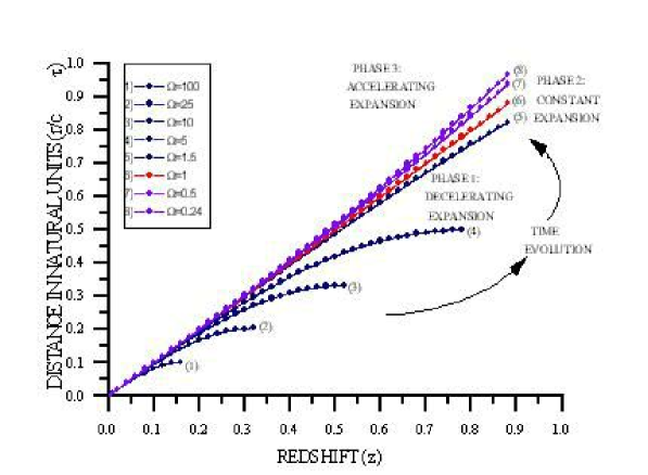
Fig. 1.:

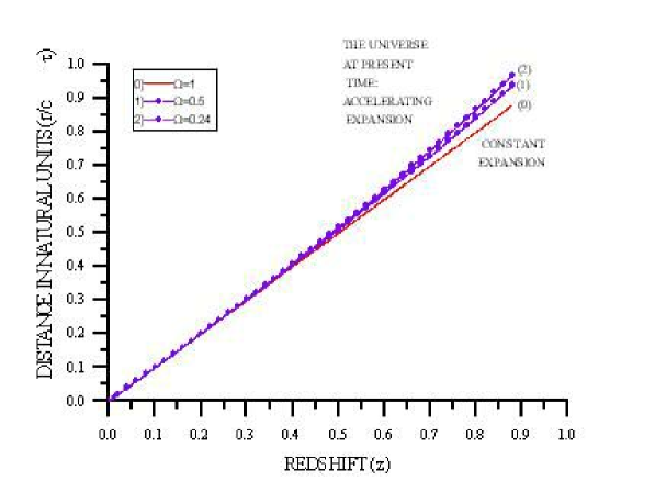
Fig. 2.:

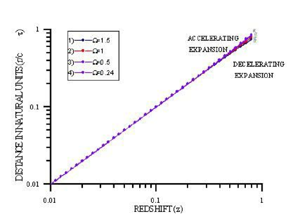
Fig. 3.:

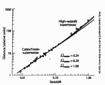
Fig. 4.:

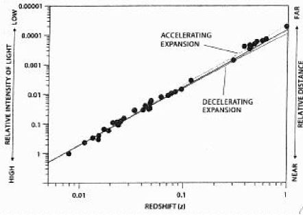
Fig. 5.:

REFERENCES

-
[1]
1. A. Friedmann, Z. Phys. 10, 377 (1922).
2. A. Friedmann, Z. Phys., 21, 326 (1924).
3. E.P. Hubble, Proc. Nat. Acad. Sci. 15, 168 (1927).
4. E.P. Hubble, The Realm of the Nebulae (Yale University Press, New Haven, 1936); reprinted by Dover Publications, New York, 1958.
5. See, for example, A. Sommerfeld, Thermodynamics and Statistical Mechanics (Academic Press, New York, 1956).
6. L.D. Landau and E.M. Lifshitz, The Classical Theory of Fields (Pergamon Press, Oxford, 1979).
7. H. Ohanian and R. Ruffini, Gravitation and Spacetime (W.W. Norton, New York, 1994).
8. M. Carmeli, Classical Fields: General Relativity and Gauge Theory (John Wiley, New York, 1982).
9. A. Papapetrou, Lectures on General Ralativity (D. Reidel, Dordrecht, The NetherLands, 1974).
10. For more details on the geometrical meaning, see D.J. Struik, Lectures on Classical Differential Geometry (Addison-Wesley, Reading, MA, 1961).
11. M. Carmeli, Found. Phys. 25, 1029 (1995); ibid., 26, 413 (1996).
12. M. Carmeli, Intern. J. Theor. Phys. 36, 757 (1997).
13. M. Carmeli, Cosmological Special Relativity: The Large-Scale Structure of Space, Time and Velocity (World Scientific, 1997).
14. M. Carmeli, Inflation at the early universe, p. 376, in: COSMO-97: First International Workshop on Particle Physics and the Early Universe, Ed. L. Roszkowski (World Scientific, 1998).
15. M. Carmeli, Inflation at the early universe, p. 405, im: Sources and Detection of Dark Matter in the Universe, Ed. D. Cline (Elsevier, 1998).
16. M. Carmeli, Aspects of cosmological relativity, pp. 155-169, in: Proceedings of the Fourth Alexander Friedmann International Seminar on Gravitation and Cosmology, held in St. Petersburg, June 17-25, 1998, Eds. Yu.N. Gnedin et al. (Russian Academy of Sciences and the State University of Campinas, Brazil, 1999); reprinted in Intern. J. Theor. Phys. 38, 1993 (1999).
17. M Carmeli, Commun. Theor. Phys. 5, 159, (1996); ibid., 6, 45 (1997).
18. W.L. Freedman, HST highlight: The extragalactic distance scale, p. 192, in: Seventeenth Texas Symposium on Relativistic Astrophysics and Cosmology, Eds. H. Böhringer et al., Vol. 759 (The New York Academy of Sciences, New York, 1995).
19. W.L. Freedman et al., Nature 371, 757 (1994).
20. M. Pierce et al., Nature 371, 385 (1994).
21. B. Schmidt et al., Astrophys. J. 432, 42 (1994).
22. A. Riess et al., Astrophys. J. 438, L17 (1995).
23. A. Sandage et al., Astrophys. J. 401, L7 (1992).
24. D. Branch, Astrophys. J. 392, 35 (1992).
25. B. Schmidt et al., Astrophys. J. 395, 366 (1992).
26. A. Saha et al., Astrophys. J. 438, 8 (1995).
27. P.J.E. Peebles, Status of the big bang cosmology, p. 84, in: Texas/Pascos 92: Relativistic Astrophysics and Particle Cosmology, Eds. C.W. Akerlof and M.A. Srednicki, Vol. 688 (The New York Academy of Sciences, New York, 1993).
28. A.G. Riess et al., Astron. J. 116, 1009 (1998).
29. C.J. Hogan, R.P. Kirshner and N.B. Suntzeff, Scien. Am. 9, 46 (January 1999).
30. A. Einstein, Autobiographical Notes, Ed. P.A. Schilpp (Open Court Pub. Co., La Salle and Chicago, 1979).