ISO-SWS calibration and the accurate modelling of cool-star atmospheres: I. Method

Abstract

A detailed spectroscopic study of the ISO-SWS data of the red giant $\alpha$ Tau is presented, which enables not only the accurate determination of the stellar parameters of $\alpha$ Tau, but also serves as a critical review of the ISO-SWS calibration.

This study is situated in a broader context of an iterative process in which both accurate observations of stellar templates and cool star atmosphere models are involved to improve the ISO-SWS calibration process as well as the theoretical modelling of stellar atmospheres. Therefore a sample of cool stars, covering the whole A0 – M8 spectral classification, has been observed in order to disentangle calibration problems and problems in generating the theoretical models and corresponding synthetic spectrum.

By using stellar parameters found in the literature large discrepancies were seen between the ISO-SWS data and the generated synthetic spectrum of $\alpha$ Tau. A study of the influence of various stellar parameters on the theoretical models and synthetic spectra, in conjunction with the Kolmogorov-Smirnov test to evaluate objectively the goodness-of-fit, enables us to pin down the stellar parameters with a high accuracy: T_eff $=3850\pm 70$ K, $\log$ g$=1.50\pm 0.15$, M $=2.3\pm 0.8$ M_⊙, z $=-0.15\pm 0.20$ dex, $\xi_{t}$ $=1.7\pm 0.3$ $\rm{km\,s^{-1}}$, $\mathrm{{}^{12}C/^{13}C}$ $=10\pm 1$, $\varepsilon$(C) $=8.35\pm 0.20$ dex, $\varepsilon$(N) $=8.35\pm 0.25$ dex, $\varepsilon$(O) $=8.83\pm 0.15$ dex and $\theta_{d}$ $=20.77\pm 0.83$ mas. These atmospheric parameters were then compared with the results provided by other authors using other methods and/or spectra.

1 Introduction

The modelling and interpretation of the ISO-SWS (Infrared Space Observatory - Short Wavelength Spectrometer) data require an accurate calibration of the spectrometers (Schaeidt et al. 1996). In the SWS spectral region (2.38 – 45.2 $\mu$m) the primary standard calibration candles are bright, mostly cool, stars. The better the behaviour of these calibration sources in the infrared is known, the more accurate the spectrometers can be calibrated. ISO offered the first opportunity to obtain continuous mid-infrared spectra between 2.38 and 45.2 $\mu$m at a spectral resolving power of $\sim 1500$, not polluted by any molecular absorptions of the earth’s atmosphere. Therefore our knowledge on the mid-infrared behaviour of the stellar calibration sources is limited. Refining the synthetic reference spectra used to calibrate the SWS can only be done by refining the model atmospheres of the stars. A full exploitation of the ISO data can therefore only result from an iterative process in which both accurate observations and new modelling are involved. In order to obtain a reliable convergence in such an iterative process, one needs: (1) a sample of bright stellar objects spread over a large range in spectral type; (2) a thorough understanding of cool star atmospheres and of the influence of the various parameters — e.g. T_eff, $\log$ g, and chemical composition — on the emergent spectra. With this in mind, stars with spectral types ranging from A0 – M8 were observed with ISO-SWS. It is important to cover a broad parameter space in order to distinguish calibration problems from problems related to the model and/or in the generation of the synthetic spectrum. Concerning point 2 above, it is necessary to perform an intensive study of the influence of different stellar parameters on synthetic spectra. The results of such a study will be presented with the red giant $\alpha$ Tau as a test case. The results for 15 other stars in our sample will be presented in forthcoming papers.

This research has been done within the framework of the proposal STARMOD (Title: Accurate modelling of cool-star atmospheres; P.I.: C. Waelkens; C.I.: M. Cohen, L. Decin, Th. de Graauw, L.B.F.M. Waters) and the ZZSTARM proposal (Title: Accurate modelling of cool-star atmospheres; P.I.: L. Decin; C.I.: M. Cohen, C. Waelkens, Th. de Graauw, L.B.F.M. Waters). Some calibration data have been provided by the SWS Instrument Dedicated Team (SIDT) in the framework of a quick-feedback refining of the model Spectral Energy Distribution (SED) of the calibration sources used for the SWS calibration.

So far, the analysis of the discrepancies between the ISO-SWS data and the corresponding synthetic spectra has been restricted to the wavelength region from 2.38 to 12 $\mu$m, since the lack of comprehensive molecular and atomic line lists hamper fast progress at longer wavelengths (12 – 45 $\mu$m). Furthermore the brightness of the stars drops quickly in this wavelength region so that the same signal to noise ratio will not be achieved. A third point is that the SEDs may also be affected by unknown circumstellar contribution.

This paper is organized as follows: in Sect. 2 the observations are described and the data reduction procedures are discussed. In Sect. 3 a summary of the literature concerning $\alpha$ Tau is presented, on the basis of which the starting values for our modelling stellar parameters are selected. The effect of changing stellar parameters on the synthetic spectra of K and M giants is analyzed in Sect. 4. In Sect. 5 the method of analysis is outlined, while in Sect. 6 the results are discussed. In the last section, Sect. 7, the main conclusions are summarized.

2 Observations and data reduction

A full scan observation of $\alpha$ Tau has been obtained in the 2.38 – 45.2 $\mu$m wavelength range with the Short-Wavelength Spectrometer (SWS) (de Graauw et al. 1996) on board ISO. This has been done by use of the SWS observing mode AOT01 (= a single up-down scan for each aperture/order combination) with scanner speed 4, resulting in a resolving power of $\sim$ 1500. The observation lasted for 6650 s and was performed during revolution 636.

The data were processed to a calibrated spectrum sampled in all the pixels, the so-called Auto-Analysis product, using the procedures and calibration files of the ISO off-line pipeline version 7.0. For a description of the flux and wavelength calibration, we refer to Schaeidt et al. (1996) and Valentijn et al. (1996). This reduction resulted in an oversampled spectrum for each of the four AOT-bands, which each consist of 12 detectors.

Remaining instrumental effects, such as fringes in the 12.0 – 29.5 $\mu$m part of the spectrum, were removed using the SWS Interactive Analysis package (IA) provided by the SIDT. The band-2 data (4.08 – 12 $\mu$m) are severely affected by detector memory effects. Time and flux dependent memory effects occur for all four instruments (SWS, LWS, PHOT, CAM) on board ISO. So far, several attempts have been made to model the corrections of the transient effects (see e.g. Van Malderen et al. 1999), but currently no foolproof method exists to correct the SWS data for these transient effects. Memory effects appear to be less severe in the down-scan measurements, which are obtained after the up-scan data, suggesting a more stabilized response to the flux level for down-scan data. The SWS flux calibration of band 2 was corrected for a regime where the flux history of the detectors is comparable to the second scan in the observation, the so-called down scan. We therefore used the down-scan data of our observation as a reference to do a correction of the flux level of the first scan.

Several procedures were performed on each sub-band separately to combine the twelve detectors. A sigma-clipping procedure (with $\sigma=2.0$) was used to reduce the noise by discarding the datapoints in every resolution element for which the difference to the mean was $>2\sigma$. After aligning the twelve different detector signals to their average level and rebinning to the expected resolution (see Table 1), the final result was obtained. Although the resolution changes in within one sub-band, the resolution was kept constant (see Table 1) and the value was taken to be the lowest value in Fig. 6 by Lorente (1998). The individual sub-band spectra, when combined into a single spectrum, can show jumps in flux levels at the band edges. This is due to imperfect flux calibration or wrong dark-current subtraction for low-flux observations. Using the overlap regions of the different sub-bands and looking at other SWS observations, several sub-bands were multiplied by a small factor (see Table 1) to construct a smooth spectrum. Due to the problems with memory effects in band 2, the factor of band 2b was determined by use of the template of Cohen et al. (1992) and the obtained synthetic spectra. Note that all shifts are well within the photometric absolute calibration uncertainties claimed by Schaeidt et al. (1996).

Table 1: Resolution and factors used to shift the sub-bands.

	wavelength
sub-band	range [$\mu$m]	resolution	factor
1a	2.38 – 2.60	1300	1.00
1b	2.60 – 3.02	1200	1.01
1d	3.02 – 3.52	1500	1.00
1e	3.52 – 4.08	1000	1.00
2a	4.08 – 5.30	1200	1.00
2b	5.30 – 7.00	800	1.045
2c	7.00 – 12.0	800	1.00

3 Literature study: $\alpha$ Tau

Table 2: Literature study of $\alpha$ Tau, with the effective temperature T_eff given in K, the mass M in M_⊙, the microturbulent velocity $\xi_{t}$ in $\rm{km\,s^{-1}}$, the angular diameter $\theta_{d}$ in mas, the luminosity L in L_⊙ and the radius R in R_⊙. Angular diameters deduced from direct measurements (e.g from interferometry) are written in italic, while others (e.g. from spectrophotometric comparisons) are written upright.

Teff	$\log$ g	M	$\xi_{t}$	[Fe/H]	$\varepsilon$(C)	$\varepsilon$(N)	$\varepsilon$(O)	12C/13C	$\theta_{d}$	L	R	Ref.
$3910\pm 200$	$1.59\pm 0.30$		$2.1\pm 0.5$	$-0.34\pm 0.21$								1.
$4140\pm 100$	$1.01\pm 0.46$		$2.00\pm 0.25$	$-0.33\pm 0.18$	$8.27\pm 0.18$	$7.46\pm 0.28$	$8.60\pm 0.24$	$9\pm 1$		200		2.
									21.154			3.
$3860\pm 100$	$1.5\pm 0.5$		$2.2\pm 0.7$		$8.39\pm 0.05$							4.
$3860\pm 100$	$1.5\pm 0.5$		$2.2\pm 0.7$		$8.31\pm 0.03$							4.
$3860\pm 100$	$1.5\pm 0.5$		$2.20\pm 0.14$		$8.37\pm 0.14$							5.
$3850\pm 100$	$1.5\pm 0.3$	1.5	$1.9\pm 0.3$	$0.00\pm 0.20$	$8.38\pm 0.08$	$8.35\pm 0.06$	$8.77\pm 0.08$	10				6.
3831	1.41	1.5	2.0		8.37			$9\pm 1$				7.
$3830\pm 100$	$1.2\pm 0.4$	1.4	2.1	$-0.14$				$\sim 12$	24	413 [$463\pm 59$]	$49\pm 4$	8.
3790	1.8							12				9.
3898	2.0								$21.32\pm 0.58$			10.
3800	1.8		1.0	$-0.17\pm 0.14$								11.
$3970\pm 70$	$1.3\pm 0.35$	$1.5^{+3.0}_{-1.0}$	1.9	0.00					23	$414\pm 75$		12.
3789	1.8		1.5					$12\pm 2$				13.
$3875\pm 100$	1.55	1.0	$2.2\pm 0.5$	$+0.16\pm 0.20$	$8.73\pm 0.20$	$8.61\pm 0.10$	$9.02\pm 0.10$	$15^{+5}_{-10}$				14.
$3875\pm 100$	0.55	1.0	$2.2\pm 0.5$	$-0.16\pm 0.20$	$8.26\pm 0.20$	$7.95\pm 0.10$	$8.60\pm 0.10$	$15^{+5}_{-10}$				14.
$3860\pm 100$	$1.5\pm 0.5$		$2.5\pm 1.0$		$8.39\pm 0.05$	$8.05\pm 0.25$						15.
$3940\pm 50$	$1.25\pm 0.49$		$2.2\pm 0.2$	$-0.14\pm 0.30$								16.
3950	1.5 [1.3]		1.5 [2.0]	0.00			$8.97$ [9.03]					16.
3850	0.9 [0.6]		1.5 [2.0]	$-0.5$			8.47 [8.53]					16.
3750	0.5 [0.2]		1.5 [2.0]	$-0.5$			8.27 [8.37]					16.
									${\mathit{20.88\pm 0.10}}$			17.
$3970\pm 49$									$20.21\pm 0.30$			18a.
$3859\pm 31$									21.07			18b.
									${\mathit{21.205\pm 0.21}}$			19.
									${\mathit{\theta_{\mathrm{UD}}=19.88\pm 0.14}}$			20.
									${\mathit{\theta_{\mathrm{UD}}=19.80\pm 0.12}}$			20.
$3976\pm 485$										$417\pm 83$	$43.0\pm 4.4$	21.
$3920\pm 15$									20.634			22.
3690												23.
3943	1.2			$-0.10$					20.62			24.
				$-0.102\pm 0.038$								25.
$3790\pm 200$	$2.2\pm 0.3$			$-0.22\pm 0.3$								26.
									20.0–35.0		23.0	27a.
									16.0–24.0		45.0–52.0	27b.
$3947\pm 41$									${\mathit{20.44\pm 0.11}}$			28.
3840									21.4			29.
3820									$20.3\pm 1.4$			30.
$3490\pm 150$									$21.6\pm 1.9$			31.
4000									$21.4\pm 1.1$			32.
$3850\pm 100$	$1.5\pm 0.3$	1.5	$1.9\pm 0.3$	$0.00\pm 0.20$	$8.40\pm 0.20$	$8.20\pm 0.20$	$8.78\pm 0.20$	$10$				33.

1. McWilliam 1990; 2. Lambert & Ries 1981; 3. Blackwell et al. 1990; 4. Tsuji 1991; 5. Tsuji 1986; 6. Smith & Lambert 1985; 7. Harris & Lambert 1984; 8. Kovács 1983; 9. Lambert et al. 1980; 10. Cohen et al. 1996b; 11. Fernández-Villacañas et al. 1990; 12. van Paradijs & Meurs 1974; 13. Tomkin & Lambert 1974; 14. Luck & Challener 1995; 15. Aoki & Tsuji 1997; 16. Bonnell & Bell 1993; 17. Ridgway et al. 1982; 18a. Di Benedetto & Rabbia 1987; 18b. Di Benedetto 1998; 19. Mozurkewich et al. 1991; 20. Quirrenbach et al. 1993; 21. Volk & Cohen 1989; 22. Blackwell et al. 1991; 23. Linsky & Ayres 1978; 24. Bell & Gustafsson 1989; 25. Taylor 1999; 26. Burnashev 1983; 27^a,b. Fracassini et al. 1988; 28. Perrin et al. 1998; 29. Engelke 1992; 30. Blackwell & Shallis 1977; 31. Scargle & Strecker 1979; 32. Manduca et al. 1981; 33. Smith & Lambert 1990

$\alpha$ Tau (= HD 29139 = HR 1457 = HIC 21421) is classified as a K5III giant. A detailed literature study was necessary, on the one hand to extract the best possible set of starting fundamental parameters in order to reduce the number of calculated spectra and on the other hand to check the consistency between the stellar parameters deduced from the ISO-SWS data and other spectra/methods. An exhaustive discussion of published results is presented in Table 2 and in Appendix A.

After evaluation of the various sources, the stellar parameters of McWilliam (1990), with T_eff = 3900 K, $\log$ g = 1.60, $\xi_{t}$ = 2.0 $\rm{km\,s^{-1}}$, [Fe/H] = $-0.30$, together with $\varepsilon$(C) = 8.27, $\varepsilon$(N) = 7.86, $\varepsilon$(O) = 8.60 (Lambert & Ries (1981), but with [N/Fe] taken to be $+0.20$ according to Luck & Challener (1995), see Appendix A), a mass of 1.5 M_⊙ (van Paradijs & Meurs 1974), the limb-darkened angular diameter $\theta_{d}$ $=20.88$ mas from Ridgway et al. (1982) and $\mathrm{{}^{12}C/^{13}C}$ $=10$ (Smith & Lambert 1985) were taken as starting values. In Fig. 1 both band 1 of the ISO-SWS data of $\alpha$ Tau and the synthetic spectrum generated with these parameters are shown. From Fig. 1, it is already obvious that not only the angular diameter $\theta_{d}$ should be lowered and/or T_eff should be increased, but also other parameters may need improvement.

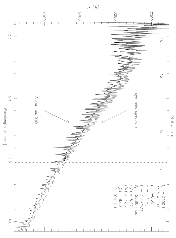
Figure 1: Comparison between band 1 of the ISO-SWS data of $\alpha$ Tau (black) and the synthetic spectrum (grey) with stellar parameters T_eff = 3900 K, $\log$ g = 1.60, M = 1.5 M_⊙, z = $-0.30$, $\xi_{t}$ = 2.0 $\rm{km\,s^{-1}}$, $\mathrm{{}^{12}C/^{13}C}$ = 10, $\varepsilon$(C) = 8.27, $\varepsilon$(N) = 7.86, $\varepsilon$(O) = 8.60 and $\theta_{d}$ = 20.88 mas.

4 Influence of stellar parameters on synthetic spectra

In this section the effect of stellar parameters on the absorption by CO, SiO, OH and H₂O is discussed. We mainly focus on these molecules since they are the most prominent absorbers for oxygen-rich giants in the wavelength range considered here (2.38 – 12 $\mu$m) (see, e.g., Fig. 2 and Fig. 3 in Decin et al. (1997) and Fig. 4 in this paper). The goal of this part of the study is to learn how the synthetic spectrum will change when one of the parameters is changed within its uncertainties, the only exception being the stellar mass and the $\mathrm{{}^{12}C/^{13}C}$ ratio due to their small influence. A simple equation for any chemical compound is not easily obtained, nor is a unique scenario able to explain all different behaviours, but some patterns do emerge. These results are then useful for the determination of the origin of the discrepancies seen between ISO-SWS data and synthetic spectra.

Since the strength of molecular (and atomic) lines is proportional to the ratio of line to continuous absorption coefficient, $l_{\nu}/\kappa_{\nu}$, approximations for this ratio are sought for. The approximate ratio is referred to as ${\cal{R}}$ and equations for some molecules have been deduced according to the approach of Kjægaard et al. (1982) (see Appendix B).

The ratio ${\cal{R}}$ has been studied for the surface flux using the following parameters:
T_eff = 3650 K – 3850 K – 4050 K
$\log$ g = 1.00 – 1.50 – 2.00
z = $-0.15$ – 0.00 – 0.15
M = 1.5 M_⊙ – 10 M_⊙ – 15 M_⊙
$\xi_{t}$ = 1.0 $\rm{km\,s^{-1}}$ – 2.0 $\rm{km\,s^{-1}}$
$\mathrm{{}^{12}C/^{13}C}$ = 10 – 4.26
$\varepsilon$(C) = 8.24 – 8.54
$\varepsilon$(N) = 8.26 – 8.56
$\varepsilon$(O) = 8.83 – 9.13

All computed spectra are compared with the synthetic spectrum with parameters: T_eff = 3650 K, $\log$ g = 1.00, z = 0.00, M = 1.5 M_⊙, $\xi_{t}$ = 2.0 $\rm{km\,s^{-1}}$, $\mathrm{{}^{12}C/^{13}C}$ = 10, $\varepsilon$(C) = 8.24, $\varepsilon$(N) = 8.26, $\varepsilon$(O) = 8.83. If not specified these stellar parameters are used. In Fig. 2 the overall results of a change $\Delta$T_eff = 200 K (a), $\Delta\log$ g = 0.50 (b), $\Delta$M = 13.5 M_⊙ (c), $\Delta$z = 0.15 (d), $\Delta$$\xi_{t}$ = 1.0 $\rm{km\,s^{-1}}$ (e), $\Delta$$\mathrm{{}^{12}C/^{13}C}$ = 5.84 (f), $\Delta\varepsilon$(C) = 0.30 (g), $\Delta\varepsilon$(N) = 0.30 (h), $\Delta\varepsilon$(O) = 0.30 (i) are shown. The results mentioned and discussed in this study apply only to models with similar stellar parameters.

Figure 2: Division of the synthetic spectrum with parameters T_eff = 3650 K, $\log$ g = 1.00, M = 1.5 M_⊙, z = 0.00, $\xi_{t}$ = 2.0 $\rm{km\,s^{-1}}$, $\mathrm{{}^{12}C/^{13}C}$ = 10, $\varepsilon$(C) = 8.24, $\varepsilon$(N) = 8.26, $\varepsilon$(O) = 8.83 by the synthetic spectrum with the same parameters but with (a) T_eff  = 3850 K, (b) $\log$ g = 0.50, (c) M = 15 M_⊙, (d) z = 0.15, (e) $\xi_{t}$ = 1 $\rm{km\,s^{-1}}$, (f) $\mathrm{{}^{12}C/^{13}C}$ = 4.26, (g) $\varepsilon$(C) = 8.54, (h) $\varepsilon$(N) = 8.56 and (i) $\varepsilon$(O) = 9.13. Prominent molecular bands are specified in the plot. Plot (a) has been divided by the factor $3650/3850$ to compensate for the higher flux of the spectrum with an effective temperature of 3850 K.

4.1 Models

The models and corresponding synthetic spectra have been computed by using the MARCS-code (Gustafsson et al. 1975). Since 1975, this code has undergone some modifications, the most important ones being the replacement of the Opacity Distribution Function (ODF) technique by the Opacity Sampling (OS) technique, the possibility to use a spherically symmetric geometry for extended objects and major improvements of the line and continuous opacities (Plez et al. 1992).

The common assumptions of spherical or plane-parallel stratification in homogeneous stationary layers, hydrostatic equilibrium and LTE were made. Energy conservation was required for radiative and convective flux, where the energy transport due to convection was treated through a local mixing-length theory (Henyey et al. 1965). The mixing-length $l$ was chosen as 1.5 $H_{p}$, with $H_{p}$ the pressure scale height, which is a reasonable quantity to simulate the temperature structure beneath the photosphere (Nordlund & Dravins 1990). Turbulent pressure was neglected. The reliability of these assumptions is discussed by Plez et al. (1992).

The synthetic spectra were generated using the TurboSpectrum program described by Plez et al. (1993), and further updated. The program treats the chemical equilibrium for hundreds of molecules with a consistent set of partition functions and dissociation energies. Solar abundances from Anders & Grevesse (1989) have been assumed, except for the iron abundance, $\varepsilon$(Fe)$=7.51$, which is in better agreement with the meteoritic value.

The continuous opacity sources considered here are H^-, H, Fe, (H+H), H${}_{2}^{+}$, H${}_{2}^{-}$, He I, He I_ff, He^-, C I, C II, C I_ff, C II_ff, C^-, N I, N II, N^-, O I, O II, O^-, CO^-, H₂O^-, Mg I, Mg II, Al I, Al II, Si I, Si II, Ca I, Ca II, H₂(pr), He(pr), e${}^{-}_{\mathrm{sc}}$, H${}^{-}_{\mathrm{sc}}$, H${}_{2\,\mathrm{sc}}$, where ‘$pr$’ stands for ‘pressure induced’ and ‘sc’ for ‘scattering’.

For the line opacity in the SWS range (2.38 – 12 $\mu$m) a database of infrared lines including atoms and molecules has been prepared. For the atomic lines the data listed by Hirata & Horaguchi (1995) have been used, for CO those by Goorvitch (1994), for SiO those by Langhoff & Bauschlicher (1993), for H₂O those by Jørgensen (1994) and Ames (Partridge & Schwenke 1997), OH lines by Sauval (Melen et al. 1995), Schwenke (1997) and Goldman et al. (1998), NH lines by Sauval (Grevesse et al. 1990; Geller et al. 1991) and CH lines by Sauval (Melen et al. 1989; Grevesse et al. 1991) and CN lines by Plez (private communication). The dissociation energy for CN was taken to be 7.76 eV. An exhaustive discussion on the accuracy and completeness of infrared spectroscopic line lists can be found in Decin (2000). From this study, a preference emerged for the H₂O line list by Ames and the OH line list by Goldman. To remove the small difference between the originally ‘vacuum’ wavelengths for the ISO observations and ‘air’ wavelengths in spectroscopic linelists above 200 nm, Edlen’s formula (Edlen 1966) was extended to the infrared.

4.2 Effect of changing the effective temperature

When the temperature increases, fewer molecules are formed resulting in a smaller line absorption coefficient. At 2.3 $\mu$m, $\kappa_{\nu}$ is primarily due to H^- free-free absorption, thus its value depends directly on the electron pressure $P_{\mathrm{e}}$. Increasing the temperature causes more ionization events and thus more free electrons, but at the same time the H^- ion itself is less easily formed. Fig. 3a. shows that, for the models under consideration, this latter effect is the most important one and so $\kappa_{\nu}$ decreases when the effective temperature is increased from 3650 K to 3850 K. Moving inwards from the outer photosphere, the line absorption coefficient l_ν of all molecules (not H^-) reaches its maximum at the location where the effect of an increasing temperature overtakes the effect of a higher density. The partial pressure p of H^-, being proportional to $p$(H I)*$P_{\mathrm{e}}$, keeps on rising because of the increase of the number of free electrons at higher temperature. When the line-to-continuum contrast has to be known, one has to consider the partial pressure of the molecule divided by ($p$(H I)*$P_{\mathrm{e}}$) (see Fig. 2 and Fig. 3b). The simple statement that there are weaker absorption bands for higher temperatures does not always hold: the approximate ratio ${\cal{R}}$ of CO, SiO, OH and H₂O decreases, but for CN the lower continuous opacity compensates for the lower line opacity (see Fig. 3b). Furthermore, the relative population of rotational levels strongly depends on T (the maximum population occurs at a J_max-value and a lower T corresponds to a lower J_max-value). Therefore a given line (J) intensity could be increased or decreased according to its J-value only.

Figure 3: Comparison between the partial pressure of several molecules for the models with T_eff = 3650 K (full line) and T_eff = 3850 K (dashed line) and with $\log$ g = 1.00, M = 1.5 M_⊙, z = 0.00, $\xi_{t}$ = 2.0 $\rm{km\,s^{-1}}$, $\mathrm{{}^{12}C/^{13}C}$ = 10, $\varepsilon$(C) = 8.24, $\varepsilon$(N) = 8.26, $\varepsilon$(O) = 8.83. In plot (a) the partial pressure of the molecules is given, while in plot (b) the partial pressure of the molecules is divided by $p$(H I)*$P_{\mathrm{e}}$.

4.3 Effect of changing the gravity and the mass

Although g and M are closely related, the effect of changing the mass is smaller than that of changing the gravity, because the first one only affects the extension and the latter one also changes the pressure structure of the atmosphere. This is clearly visible in Fig. 2. The assumption of hydrostatic equilibrium links the gas pressure to the surface gravity. In a cool star, the gas and electron pressure ($P_{\mathrm{g}}$ and $P_{\mathrm{e}}$) can be written as:

$$P_{\mathrm{g}} \approx constant\cdot g^{p}\ \ {\footnotesize{(0.59\leq p\leq 1.05)}}$$ (1)

$$P_{\mathrm{e}} \approx constant\cdot g^{p}\ \ {\footnotesize{(0.20\leq p\leq 1.03)}}.$$ (2)

Due to the higher extension of the atmospheres considered here, this value of $p$ has a larger range compared to the value discussed by Gray (1992).

When the gravity increases, the electron pressure increases rapidly (Eq. 2), resulting in a higher H^- free-free absorption. Other effects of increasing the gravity are higher number densities supporting the molecular formation and the fact that molecules can be formed till higher temperatures, both increasing $l_{\nu}$. The final result is that the approximate absorption coefficient ${\cal{R}}$ can either increase or decrease depending on the relative change of l_ν and $\kappa_{\nu}$.

Using the approximate relations according to Kjærgaard et al. (1982) (see Appendix B), the conclusion is reached that an increase of gravity leads to a decrease of the strength of the CO, NH and CN lines and to an increase of the strength of the H₂O lines, with no dependence for the OH and SiO lines. The increasing gravity does lead to a strengthening of the H₂O lines and also of the OH lines while it diminishes the ${l_{\nu}}/{\kappa_{\nu}}$ ratio of CO, NH, SiO and CN (Fig. 2). From the approximate relations for ${\cal{R}}$ no quantitative conclusion on the parameter dependence can thus be made.

An increase in mass yields the inverse (but smaller) effect on the partial pressure (and so on the line absorption coefficient $l_{\nu}$) as an increase in gravity.

4.4 Effect of changing the metallicity

For the computations with a higher metallicity, [atom/H] has been increased from 0.00 dex to 0.15 dex for all atoms except for H, He, C, N and O. Because an increase in metal abundance leads to a decrease in gas pressure at each optical depth (as $\kappa_{\nu}$ increases), the partial pressures of the molecules CO, OH, N₂, H₂O and CN consequently decrease, while p(SiO) and p(TiO) are somewhat higher because of the higher abundance of Si and Ti respectively. An increase in the overall metal abundance increases the amount of electrons ($P_{\mathrm{e}}$) and as a consequence also the value of $\kappa_{\nu}$ formed by H^-. This increase of $\kappa_{\nu}$ dominates the changes in the spectrum: all molecular features become fainter at increased metallicities (with C, N and O kept constant) (Fig. 2). This can also be seen in the equations for ${\cal{R}}$ (see appendix B) for the extreme case in which all carbon is present in the form of CO with T${}_{{\mathrm{e\rm{ff}}}}\leq 4500$ K. The strong metallicity dependence of H₂O in the approximate relation for ${\cal{R}}$ may be well visible, though this increase (with decreasing z) is small for weak H₂O bands.

4.5 Effect of changing the microturbulent velocity

The impact of changing the microturbulent velocity is most important for the CO lines with a large equivalent width. When a line is saturated, increasing $\xi_{t}$ widens the wavelength range covered by the absorption and reduces the saturation, thus increasing the total absorption. In the line center of an unsaturated line, a smaller microturbulence corresponds to a higher absorption coefficient at that frequency (see Fig. 2).

Decreasing the microturbulent velocity from 2 $\rm{km\,s^{-1}}$ to 1 $\rm{km\,s^{-1}}$ diminishes the CO first overtone absorption by maximum 10% and the CO fundamental by up to 6 %, the SiO first overtone by up to 4 %, and the SiO fundamental by up to 3 %, the fundamental band of OH by up to 3 % and the ro-vibrational stretching modes ($\nu_{1}$ and $\nu_{3}$) and bending mode ($\nu_{2}$) of H₂O by up to 0.5 %.

4.6 Effect of changing the isotopic ratio $\mathrm{{}^{12}C/^{13}C}$

Red giant atmospheres display altered C, N, and O abundances and isotopic ratios (in particular $\mathrm{{}^{12}C/^{13}C}$), due to dredge-up episodes. Suppose that the $\mathrm{{}^{12}C/^{13}C}$ ratio is changed from 10 (case I) to 4.26 (case II). If a ¹²CO line is saturated in case I, its equivalent width will decrease very few from case I to case II. If we assume the ¹³CO line to be very weak in case I, its equivalent width will increase very much from case I to case II by a factor nearly equal to the new/old isotopic ratio. Therefore it is understandable that a decrease in $\mathrm{{}^{12}C/^{13}C}$ will consequently cause ${\cal{R}}$(CO) to increase, although this increase may be very small if the CO bands are weak (Fig. 2).

4.7 Effect of changing $\varepsilon$(C), $\varepsilon$(N) or $\varepsilon$(O)

When the ratio C/O increases (but remains $<$ 1), the structure of the atmosphere is affected through changes in line blanketing. More CO will be formed and less oxygen will be left (after CO formation) to form oxygen-based molecules. Hence, as illustrated in Fig. 2, the total absorption of CO will increase, while it will decrease for SiO, OH and H₂O. Increasing the oxygen abundance gives roughly the reverse effect, but the total CO absorption hardly changes. The largest effect of an increasing nitrogen abundance is an increase of the NH and CN line strengths.

5 Method of analysis

Figure 4: Relative importance of atoms and molecules in a model with T_eff = 3850 K, $\log$ g = 1.00, M = 1.5 M_⊙, z = 0.00, $\xi_{t}$ = 2.0 $\rm{km\,s^{-1}}$, $\mathrm{{}^{12}C/^{13}C}$ = 10, $\varepsilon$(C) = 8.24, $\varepsilon$(N) = 8.35, $\varepsilon$(O) = 8.83.

Fig. 1 reveals several discrepancies. As outlined in Sect. 1, the origin of these discrepancies can be either a calibration problem or a problem related to the generation of the synthetic spectrum. Precisely because this research involves both theoretical developments on the model spectra and calibration improvements of the spectral reduction method, one has to be extremely careful not to confuse technical detector problems with astrophysical issues. Therefore, several points have to be taken into account when scrutinizing these discrepancies.

First of all, one has to take into account that the calibration process is a delicate one. Due to the high flux level of the observations, dark-current subtraction does not influence the final spectrum much, but memory effects affect the reliability of band-2 observations. Therefore, mainly the band-1 data were used for the determination of the stellar parameters. The final result is however very sensitive to the Relative Spectral Response Function (RSRF) used. The RSRF was intensively measured in the lab before launch by use of a cryogenic blackbody source with temperatures between 30 and 300K. After the launch of ISO these intermediate RSRFs were corrected for broad-band residues detected by comparing reference spectral energy distributions (SEDs) — synthetic spectra (Kurucz 1993; van der Bliek et al. 1998) and composites of M. Cohen (Cohen et al. 1992, 1996a; Witteborn et al. 1999) — with SWS observations processed with these intermediate RSRFs using stellar candles of different IR spectral signature. By using a cubic spline smoothing algorithm and sigmaclipping the risk was minimized of introducing false spectral features and one also avoids possible bias by spectral features of one type of source (Vandenbussche, 1999). The absolute flux level is determined by use of photometric data and composite SEDs of various sources. The flux calibration accuracy is estimated to be 5 – 7 % in band 1, 7 – 12 % in band 2a, 7 – 15 % in band 2b and 11 – 25 % in band 2c, the worst accuracy being located at the edges. The spectral cover from A0 – M7 was highly necessary, since the different structures of the various selected stars make it possible to decide upon the quality of the used RSRFs. To test our findings, high-resolution observations of two stars were also studied in detail. For a discussion about the quality of the RSRFs, we refer to the forthcoming papers which will describe the other 15 stars in our sample.

In order to elucidate problems with the theoretical atmospheric structure, it is important to know the relative importance of the different molecules (see Fig. 4) and the influence of the stellar parameters on the total absorption by these molecules (see Sect. 4). Fig. 4 shows clearly that especially the molecules CO, OH and SiO are helpful in determining the atmospheric parameters. In spite of the moderate resolution of ISO-SWS, we will demonstrate that one can pin down the stellar parameters of cool giants very accurately from these data. This is due to the large wavelength range of ISO-SWS, where different important molecules determine the spectral signature. Since these different spectral features do each react in another way on a change of one of the several heterogeneous stellar parameters, it is possible to improve on the stellar parameters. Using a metallicity of z $=-0.30$ yields, e.g., a synthetic spectrum which has too low a flux density in the wavelength range from 2.6 – 2.8 $\mu$m, with the line contrast ${l_{\nu}}/{\kappa_{\nu}}$ being too strong. Fig. 2 turned out to be extremely useful to ascertain the gravity: the inverse influence of the gravity on the OH lines compared to the CO and SiO lines, together with the steep slope in band 1B and band 1D make it possible to pin down the logarithm of the gravity within 0.15 dex! Because the microturbulent velocity $\xi_{t}$ does not only act on the CO lines, but also on the strongest SiO and OH lines, one may disentangle a wrong microturbulence and a wrong carbon abundance.

In order to achieve the highest possible agreement between the data and the different synthetic spectra, a statistical approach is proposed. A choice was made for the Kolmogorov-Smirnov test. This well-developed goodness-of-fit criterion is applicable for a broad range of comparisons between two samples, where the kind of differences which occur between the samples can be very diverse. An elaborate discussion about the Kolmogorov-Smirnov statistics can be found in Pratt & Gibbons (1981) and Hájek (1969). In this goodness-of-fit test a parameter, $V_{k}$, is defined in the present case as the ratio of the ISO-SWS flux to the synthetic flux at frequency point $\nu_{k}$. These parameters $V_{k}$ are assumed to be independent random variables with $E\{V_{k}\}=1$ and $E\{V_{k}^{2}\}=\sigma^{2}$, with a constant unspecified variance $\sigma^{2}$. The random variables

$$Y_{i}\equiv\frac{\sum\limits_{k=1}^{i}V_{k}}{\sum\limits_{k=1}^{n}V_{k}} (i=1,\ldots,n-1)$$ (3)

(with $n$ the total number of frequency points) are then asymptotically behaving like $i/n$ and hence are asymptotically equidistributed on the interval $[0,1]$. These variables $Y_{i}$ will be formally compared with the quantiles of the uniform distribution $F(x)=x$, $0\leq x\leq 1$, using a modification of the Kolmogorov-Smirnov test. Taking the unspecified distribution function of the sample $Y_{1},\ldots,Y_{n}$ as $G$, the null hypothesis is $F=G$. The Kolmogorov-Smirnov test is based on the maximum difference. Specifically, the test statistics are given by

$$D_{nn}=\max_{t}|G_{n}(t)-F_{n}(t)|.$$ (4)

One rejects $F=G$ if $D_{nn}$ is ‘too large’ in comparison to an appropriate critical value.

Practically, our modification involves the calculation of the value $\beta$, defined as

$$\beta\equiv\sqrt{n}\sup\limits_{1\leq i\leq n-1}\left|Y_{i}-\frac{i}{n}\right|.$$ (5)

Firstly, we will compute the asymptotical distribution function of $\beta$. By defining

$$X_{i}=\frac{V_{i}-1}{\sigma},$$ (6)

one has that $E\{X_{i}\}=0$ and $E\{X_{i}^{2}\}=1$. So,

$$\beta\equiv\sqrt{n}\sup\limits_{1\leq i\leq n-1}\left|Y_{i}-\frac{i}{n}\right|=\sqrt{n}\sup\limits_{1\leq i\leq n-1}\left|\frac{\sum\limits_{k=1}^{i}V_{k}}{\sum\limits_{k=1}^{n}V_{k}}-\frac{i}{n}\right|$$ (8)

$$=\sqrt{n}\sup\limits_{1\leq i\leq n-1}\left|\frac{\displaystyle\frac{\sigma}{n}\sum\limits_{k=1}^{i}X_{k}-\frac{i}{n}\left(\frac{\sigma}{n}\sum\limits_{k=1}^{n}X_{k}\right)}{\displaystyle 1+\frac{\sigma}{n}\sum\limits_{k=1}^{n}X_{k}}\right|.$$

By defining $k\equiv[nt]$, where $[nt]$ is the greatest integer less than or equal to $nt$, Eq. (8) becomes

$$\beta=\sup\limits_{0\leq t\leq 1}\left|\frac{\displaystyle\frac{\sigma}{\sqrt{n}}\sum\limits_{k=1}^{[nt]}X_{k}-\frac{[nt]}{n}\left(\frac{\sigma}{\sqrt{n}}\sum\limits_{k=1}^{n}X_{k}\right)}{\displaystyle 1+\frac{\sigma}{n}\sum\limits_{k=1}^{n}X_{k}}\right|.$$ (9)

Using the strong law of large numbers

$$\lim_{n\to\infty}\frac{1}{n}\sum_{k=1}^{n}X_{k}=0,\qquad\textrm{almost surely}$$ (10)

and Donsker’s theorem (Billingsley, 1968, p. 137)

$$\frac{1}{\sqrt{n}}\sum_{k=1}^{[nt]}X_{k}\stackrel{{\scriptstyle\mathcal{D}}}{{\to}}W(t),$$ (11)

where $W(t)$, $0\leq t\leq 1$, is standard Brownian motion, i.e., $W(t)$ is a Gaussian process with $W(0)=0$, independent increments, and $W(t)-W(s)$ has a normal distribution with mean zero and variance $|t-s|$, one sees that $\beta$ converges in distribution to

$$\beta\stackrel{{\scriptstyle\mathcal{D}}}{{\to}}\sigma\sup_{0\leq t\leq 1}|W(t)-tW(1)|.$$ (12)

Here $W_{0}(t)\equiv W(t)-tW(1)$, $0\leq t\leq 1$, is known as a Brownian Bridge. The definition of $W_{0}$ implies that $W_{0}$ is a Gaussian process with $E\{W_{0}(t)\}=0$ and
$E\{W_{0}(s)W_{0}(t)\}=s(1-t)$ if $s\leq t$. As a consequence

$$\beta^{*}\equiv\frac{\beta}{\sigma}\stackrel{{\scriptstyle\mathcal{D}}}{{\to}}\sup_{0\leq t\leq 1}|W_{0}(t)|,$$ (13)

which implies that the asymptotic distribution function of $\beta^{*}$ is given by the Kolmogorov-Smirnov distribution

$$P(\beta^{*}\geq\lambda)=2\sum_{i=1}^{\infty}(-1)^{i+1}\exp\{-2i^{2}\lambda^{2}\}$$ (14)

(Billingsley, 1968, p. 105). For a test with significance level $\alpha$ one rejects the null hypothesis when $\beta^{*}>\lambda_{\alpha}$, where

$$2\sum_{i=1}^{\infty}(-1)^{i+1}\exp\{-2i^{2}\lambda_{\alpha}^{2}\}=\alpha.$$

For $\alpha=0.05$ one has $\lambda_{\alpha}=1.36$ and for $\alpha=0.01$ one has $\lambda_{\alpha}=1.63$. So, a good approximation to the level-$\alpha$ Kolmogorov-Smirnov test is to reject a fit if the empirical distribution function exits from the bounds

$$y=x\pm\lambda_{\alpha}(n-1)^{-1/2},\ 0<x<1$$ (15)

(see, e.g., Fig. 10.2 in Brockwell & Davis (1991)).

The lower the $\beta$-value, the better the accordance between the observed data and synthetic spectrum. It is clear that $\beta=\sigma\beta^{*}$ gives us not only information about the correspondence between the observed and synthetic spectra, but also about $\sigma$. Since $V_{k}$ is the ratio of the ISO-SWS flux ($\cal{F}_{\mathrm{obs}}$) to the synthetic flux ($\cal{F}_{\mathrm{syn}}$), it is obvious that

$$E({\cal{F}}_{\mathrm{obs}}-{\cal{F}}_{\mathrm{syn}})^{2}={\cal{F}}_{\mathrm{syn}}^{2}\sigma^{2},$$ (16)

and thus

$$\sigma^{2}=\frac{E({\cal{F}}_{\mathrm{obs}}-{\cal{F}}_{\mathrm{syn}})^{2}}{{\cal{F}}_{\mathrm{syn}}^{2}}.$$ (17)

The unknown variance $\sigma^{2}$ is thus an indication on the variance of the observed data.

The Kolmogorov-Smirnov test globally checks the goodness of fit of the observed and synthetic spectra. An advantage of this test is that one very discrepant frequency point (e.g. due to a wrong oscillator strength) only mildly influences the final result. To avoid too high an influence of the less reliable calibration at the band edges, the parameter $\beta$ was computed for each sub-band separately. In each sub-band, several sub-intervals were considered to the main absorber in the relevant wavelength range, and the parameter $\beta$ was computed for each of this sub-intervals. The resulting ($Y-F$)-figures turned out to be very useful to reveal systematic problems (see, e.g., Fig. 5).

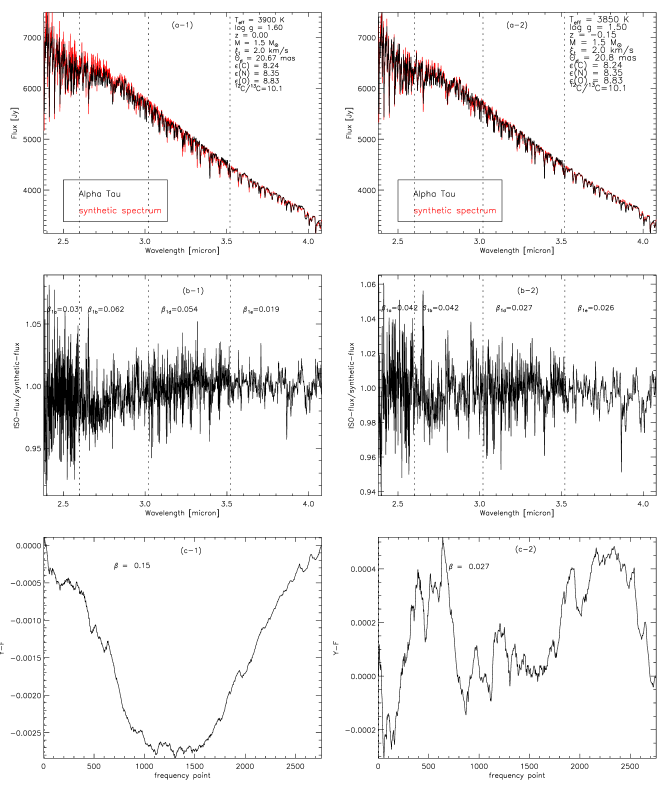
Figure 5: Fig. (a-1) shows the comparison between band 1 of the ISO-SWS data of $\alpha$ Tau (black) and the synthetic spectrum (red) with stellar parameters T_eff = 3900 K, $\log$ g = 1.60, M = 1.5 M_⊙, z = 0.00, $\xi_{t}$ = 2.0 $\rm{km\,s^{-1}}$, $\mathrm{{}^{12}C/^{13}C}$ = 10, $\varepsilon$(C) = 8.24, $\varepsilon$(N) = 8.35, $\varepsilon$(O) = 8.83 and $\theta_{d}$ = 20.67; in Fig. (a-2) the synthetic spectrum has as stellar parameters T_eff = 3850 K, $\log$ g = 1.50, M = 1.5 M_⊙, z = -0.15, $\xi_{t}$ = 2.0 $\rm{km\,s^{-1}}$, $\mathrm{{}^{12}C/^{13}C}$ = 10, $\varepsilon$(C) = 8.24, $\varepsilon$(N) = 8.35, $\varepsilon$(O) = 8.83 and $\theta_{d}$ = 20.77 mas. In Fig. (b-1) and (b-2) the ratio of the ISO-SWS flux to the synthetic flux of respectively (a-1) and (a-2) is plotted. The difference between the partial sum $Y_{i}$ and the straight line $i/n$ is plotted against the number i of the frequency point in Fig. (c-1) and Fig. (c-2). The parameter $\beta$ of the different sub-bands is indicated in Fig. (b-1) and Fig. (b-2), whereas the parameter $\beta$ of the entire band 1 is indicated in Fig. (c-1) and Fig. (c-2).

Very low $\beta$-values ($<0.09$) were achieved, proving a good relation between observed and synthetic spectra. The objective $\beta$-parameters, which are - in se - deviation estimating parameters, were then further used to improve the stellar parameters. A sensible rule of thumb would then be to select the synthetic spectrum with the lowest $\beta$-values, among those that are consistent with the null hypothesis. In addition, it is a useful sensitivity analysis to compare various spectra with acceptable $\beta$-values in key characteristics. The high flux accuracy enables us to distinguish between $\beta=0.15$ and $\beta=0.03$ (see Fig. 5), although both values are in the same region of accepting the null hypothesis. From the sensitivity analysis, it seemed to be useful to determine a maximum acceptable $\beta$-value (i.e. a minimal deviation) as an objective criterion. A synthetic spectrum is accepted to represent the true stellar parameters of $\alpha$ Tau (and the other stars) when the $\beta$-values are lower than the values given in column 2 of Table 3. These empirical $\beta_{\mathrm{max}}$-values give, as already mentioned (Eq. (17)), an indication on the uncertainty on the observational spectrum determined by e.g. the pointing accuracy, the pointing jitter of ISO, uncertainties on the RSRFs, problematic dark-current subtraction, … In Fig. 6 the standard deviation, obtained when rebinning the oversampled spectrum of $\alpha$ Tau to the expected resolution, of each bin is shown. Obviously, the ISO-SWS spectrum is less accurate in band 1A than in the other bands. This is reflected in the higher maximum acceptable $\beta$-value in Table 3. In column 3 of Table 3, the final $\beta$-values for $\alpha$ Tau are given.

Table 3: $\beta$-value for the different sub-bands and molecules in that sub-band. In the second column the maximum acceptable value is given; in the third column the correspondent value for $\alpha$ Tau.

sub-band/	maximum acceptable	$\beta$-value
molecule	$\beta$-value	for $\alpha$ Tau
1a	0.06	0.040
1b	0.05	0.034
1d	0.04	0.036
1e	0.04	0.027
CO (1a)	0.06	0.040
CO (1b)	0.05	0.039
OH (1b)	0.04	0.024
OH (1d)	0.04	0.036
OH (1e)	0.03	0.025
SiO (1e)	0.03	0.022

Figure 6: Standard deviation of the different bins, obtained when rebinning the oversampled spectrum of $\alpha$ Tau to the expected resolution.

Due to the smaller weight which are given automatically to small features, the traditional comparison between observed and synthetic spectra by eye-ball fitting is still necessary as a complement to this Kolmogorov-Smirnov method in order to reveal systematic errors in those features. The final error bars on the atmospheric parameters are then estimated from 1. the intrinsic uncertainty on the synthetic spectrum (i.e. the possibility to distinguish different synthetic spectra at a specific resolution i.e. there should be a relevant difference in $\beta$-values) which is thus dependent on both the resolving power of the observation and the specific values of the fundamental parameters, 2. the uncertainty on the ISO-SWS spectrum which is directly related to the quality of the ISO-SWS observation , 3. the value of the $\beta$-parameters in the Kolmogorov-Smirnov test and 4. the still remaining discrepancies between observed and synthetic spectrum. However, no exact formula can be given to compute the error bars due to the dependence of the several parameters. When a quantity $Q$ depends on other independent parameters, e.g. $a$ and $b$, the uncertainty $s$ is estimated from the expressions

$$s_{<Q>}\simeq\sqrt{\left(\frac{\partial Q}{\partial a}\right)^{2}s^{2}_{<a>}+\left(\frac{\partial Q}{\partial b}\right)^{2}s^{2}_{<b>}}$$ (18)

or, equivalently

$$\frac{s_{<Q>}}{Q}\simeq\sqrt{\left(\frac{1}{Q}\frac{\partial Q}{\partial a}\right)^{2}s^{2}_{<a>}+\left(\frac{1}{Q}\frac{\partial Q}{\partial b}\right)^{2}s^{2}_{<b>}}.$$ (19)

The power of the Kolmogorov-Smirnov test has already been proven in the field of astronomy, even multidimensional versions of the Kolmogorov-Smirnov test are developed for astronomical purposes (Fasano & Franceschini 1987; Gosset 1987). Fasano & Franceschini (1987) demonstrate even that the Kolmogorov-Smirnov test is a much more goodness-of-fit test than the often used $\chi^{2}$-test. It is, however, the first time that this test is used to evaluate synthetic spectra with respect to observational data.

To summarize the strategy:
1) from the large set of stars and two high-resolution observations, it is possible to indicate calibration problems (see forthcoming paper);
2) in the comparison between observed and synthetic spectrum, some discrepancies were clearly visible. The knowledge on the relative importance of the different molecules (Fig. 4) and on the influence of the various stellar parameters (Fig. 2) makes it possible to elicit the origin of these discrepancies. This is due to the presence of different molecules in this large wavelength range, whose spectral shape and strength are a very good diagnostic tool to reveal the stellar parameters;
3) once a high level of accuracy is achieved, the Kolmogorov-Smirnov test can be used for further refinement. From the ($Y-F$) plots, one can deduce systematic errors, yielding an indication on inaccurate stellar parameters. By using the results illustrated in Fig. 2, one can improve the stellar parameters. The stellar parameters, used to generate a synthetic spectrum, are taken to represent the ‘true’ stellar parameters, once the $\beta$-values are lower than a certain maximum value.

6 Discussion

Our best fit involves a synthetic spectrum with stellar parameters T_eff = 3850 K, $\log$ g = 1.50, M = 2.3 M_⊙, z = $-0.15$, $\xi_{t}$ = 1.7 $\rm{km\,s^{-1}}$, $\mathrm{{}^{12}C/^{13}C}$ = 10, $\varepsilon$(C) = 8.35, $\varepsilon$(N) = 8.35, $\varepsilon$(O) = 8.83 and $\theta_{d}$ = 20.77 mas (see Fig. 7). The uncertainties are estimated to be $\Delta$T_eff $=70$ K, $\Delta\log$ g$=0.15$, $\Delta$$\xi_{t}$ $=0.3$ $\rm{km\,s^{-1}}$, $\Delta$z $=0.20$, $\Delta\varepsilon$(C) $=0.20$, $\Delta\varepsilon$(N) $=0.25$, $\Delta\varepsilon$(O) $=0.15$, $\Delta$$\mathrm{{}^{12}C/^{13}C}$ $=1$ and $\Delta\theta_{D}=0.03$. The quoted accuracy of 0.03 mas does not take the absolute photometric flux accuracy into account, which is 5 % in band 1, resulting in $\Delta\theta_{D}<0.83$ mas.

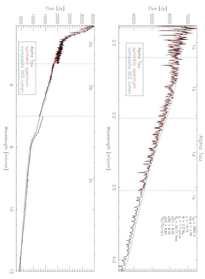
Figure 7: Comparison between band 1 and band 2 of the ISO-SWS data of $\alpha$ Tau (black) and the synthetic spectrum (red) with stellar parameters T_eff = 3850 K, $\log$ g = 1.50, M = 2.3 M_⊙, z = $-0.15$, $\xi_{t}$ = 1.7 $\rm{km\,s^{-1}}$, $\mathrm{{}^{12}C/^{13}C}$ = 10, $\varepsilon$(C) = 8.35, $\varepsilon$(N) = 8.20, $\varepsilon$(O) = 8.83 and $\theta_{d}$ = 20.77 mas. The composite SED of Cohen et al. (1992) is plotted in blue.

Due to the minor influence of the stellar mass, the uncertainty on this parameter, which follows from the construction of a synthetic spectrum, is quite large. But by using the parallax this uncertainty is constrained to $\Delta$M $=0.8$ M_⊙. The parallax measurement by Hipparcos for $\alpha$ Tau is $50.09\pm 0.95$ mas, which corresponds to a distance of $19.96\pm 0.39$ pc. With an angular diameter $\theta_{d}$ of $20.77\pm 0.83$ mas, a radius R $=44.6\pm 2.0$ R_⊙ is found, which combined with $\log$ g $=1.50\pm 0.15$, implies a mass of $2.3\pm 0.8$ M_⊙. A refinement in the mass determination was proposed by El Eid (1994), who noted a correlation between the ¹⁶O/¹⁷O ratio and stellar mass for evolved stars. Using this ratio in conjunction with evolutionary calculations, El Eid (1994) found a mass of 1.5 M_⊙ for $\alpha$ Tau. A comparison of the deduced luminosity and effective temperature with evolutionary tracks (cfr. McWilliam 1990) indicates a mass of 2.0 M_⊙ for $\alpha$ Tau.

The accuracy of the method can be tested by making a grid around the resultant final stellar parameters. This is illustrated for $\alpha$ Tau in Table 4. The $\beta$-values, corresponding to the final stellar paramters, for the different sub-bands are $\beta_{\mathrm{1A}}=0.040$, $\beta_{\mathrm{1B}}=0.034$, $\beta_{\mathrm{1D}}=0.036$, $\beta_{\mathrm{1E}}=0.027$ (see Table 3). In Table 4, the $\beta$-values are given for a change of one of the main stellar parameters, being the temperature, the gravity, the metallicity, the carbon abundance, the nitrogen abundance and the oxygen abundance. From this table, one can deduce that there are four other acceptable sets of parameters, indicated by a grey box. The final stellar parameters — as mentioned above — were chosen to represent the ‘true’ atmospheric parameters of $\alpha$ Tau, due to the lower $\beta$-value in band 1A, where the important molecule CO is absorbing.

Table 4: $\beta$-values from the Kolmogorov-Smirnov test for the evaluation of several synthetic spectra w.r.t. the ISO-SWS spectrum of $\alpha$ Tau. If not specified, the used stellar parameters were T_eff = 3850 K, $\log$ g = 1.50, $\xi_{t}$ = 1.7 $\rm{km\,s^{-1}}$, [Fe/H] = $-0.15$, $\varepsilon$(C) = 8.35, $\varepsilon$(N) = 8.35, $\varepsilon$(O) = 8.83, $\theta_{d}$ = 20.77. The $\beta$-values for these stellar parameters are given as $\beta_{\mathrm{final}}$.

	$\beta_{\mathrm{1A}}$	$\beta_{\mathrm{1B}}$	$\beta_{\mathrm{1D}}$	$\beta_{\mathrm{1E}}$
$\beta_{\mathrm{max}}\ \$	0.060	0.050	0.040	0.040
$\beta_{\mathrm{final}}$	0.040	0.034	0.036	0.027
Teff = 3710	0.080	0.050	0.059	0.027
3780	0.054	0.028	0.026	0.017
3920	0.031	0.043	0.084	0.028
3990	0.044	0.046	0.104	0.041
$\log$ g = 1.20	0.037	0.093	0.071	0.015
1.35	0.034	0.063	0.064	0.018
1.65	0.045	0.028	0.044	0.027
1.80	0.051	0.055	0.032	0.027
z = $-0.45$	0.037	0.094	0.075	0.013
$-0.30$	0.034	0.062	0.066	0.015
0.00	0.045	0.028	0.043	0.024
0.15	0.050	0.054	0.029	0.030
$\varepsilon$(C) = 8.05	0.047	0.132	0.040	0.018
8.20	0.042	0.065	0.045	0.021
8.50	0.036	0.093	0.063	0.031
8.65	0.065	0.174	0.085	0.044
$\varepsilon$(N) = 7.85	0.043	0.032	0.051	0.019
8.10	0.041	0.031	0.051	0.021
8.60	0.034	0.032	0.055	0.025
8.85	0.031	0.034	0.059	0.028
$\varepsilon$(O) = 8.63	0.057	0.049	0.096	0.046
8.73	0.035	0.040	0.075	0.034
8.93	0.052	0.019	0.026	0.018
8.03	0.070	0.043	0.028	0.019

According to Fig. 20 in Bessell et al. (1998), $\alpha$ Tau, with a ($V-K$) colour index of 3.67, has a bolometric correction BC_K of $2.60\pm 0.05$. From the bolometric magnitude $m_{\mathrm{bol}}=-0.21\pm 0.05$, the distance $d=19.964\pm 0.379$, the assumption that the interstellar extinction may be neglected, and by adapting the absolute bolometric magnitude of the Sun $M_{\mathrm{bol},\odot}=4.74$ (according to Bessell et al. 1998), one deduces the luminosity of $\alpha$ Tau L $=382\pm 23$ L_⊙. A radius R of $44.6\pm 2.4$ R_⊙ (calculated from the distance $d$ and the angular diameter $\theta_{d}$) yields an effective temperature of $3828\pm 180$ K. This is in very good agreement with the effective temperature deduced from the ISO-SWS spectrum, being T_eff $=3850\pm 70$ K. This latter T_eff, in conjunction with L $=382$L_⊙, would give R $=44.05\pm 5.55$ R_⊙ and $\theta_{d}$ $=20.53\pm 2.6$ mas.

It is clear that a gravity of $\log$ g = $1.50\pm 0.15$ dex agrees better with a ‘physical’ gravity ($\log$ g$=1.44$ from M = 2 M_⊙ and R = 44.6 R_⊙) determined by the mass M, the radius R — or the effective temperature T_eff and the luminosity L — and/or evolutionary tracks than with a ‘spectroscopic’ gravity of e.g. Lambert & Ries (1981), Kovács (1983) and Luck & Challener (1995) (see Appendix A). It is well known that the accuracy of spectroscopic determinations of gravities from ionization equilibria or molecular equilibria for individual stars is not very good for red giants (cf., e.g., Trimble & Bell 1981, Brown et al. 1983, Smith & Lambert 1985). Smith & Lambert (1985) suggested that the low spectroscopic gravity $\log$ g = 0.8 may be due to non-LTE effects on iron lines. After corrections for these effects, Smith & Lambert (1990) finally determined values for the various atmospheric parameters, with which our results agree very well. Our method for gravity determination from infrared spectra appears to be much less affected by NLTE effects, being based on a broad range of diagnostics over a large spectral interval. A great advantage of the used Kolmogorov-Smirnov test, is also that several deviation estimating parameters $\beta$ are calculated, which are not independent and are each of them related to the specific pattern of behaviour of absorption of the different molecules. E.g. the abundance of carbon is mainly determined from the band-1A and band-1B data, while a wrong gravity is traced from the $\beta_{\mathrm{1B,1D}}$-values. Simulations with other ($\log$ g, $\varepsilon$(C))-combinations never reached the same level of agreement as for the ($\log$ g = 1.50, $\varepsilon$(C) = 8.35)-combination. Using e.g. $\log$ g = 1.35 requires a lower carbon abundance (than $\varepsilon$(C) = 8.35) in order to fit the CO line strengths. The best fit then is obtained for $\varepsilon$(C) = 8.25, with $\beta_{\mathrm{1A}}$ = 0.033 and $\beta_{\mathrm{1B}}$ = 0.024. The corresponding $\beta_{\mathrm{1D}}$-value is then, however, 0.056 arising from too steep a continuum.

The mass M, luminosity L and radius R are the three fundamental parameters of a (spherical) star where two of these may be replaced by the surface gravity g = $G$M/R² and the effective temperature $\sigma$T_eff⁴=L/(4$\pi$R²). Both the mass and the luminosity are measurable physical quantities, whereas the radius of a star is a fictitious quantity because a star is a gaseous sphere and does not have a sharp edge. The relevant observable quantity is the center-to-limb variation (=clv) of intensity or limb darkening. The sun is the only star whose clv one can observe directly. Direct diameter determinations are based on a standard procedure which evaluates interferometric, lunar occultation or binary eclipse data by determining a radius position on the base of a parameterized approximation (e.g. uniform disk) of a model-predicted limb-darkening curve (see e.g. Scholz 1998). The radius is then taken at $\mu=0$ ($\mu=\cos\theta$, with $\theta$ the angle between the radius vector and the line of sight). Published limb-darkening coefficients (for an overview, see Scholz (1998)) are then needed to convert to the limb-darkened corrected angular diameter. In Table 2, this limb-darkened angular diameter is listed for the direct angular diameter determinations, except when otherwise mentioned. The angular diameter value derived by us from the ISO-SWS data is however a ‘theoretical’ radius deduced from an indirect method. It corresponds to the definition $\sigma$T_eff⁴ = L/(4$\pi$R($\tau_{\mathrm{ross}}=1$)²) and $\log$ g = GM/R($\tau_{\mathrm{ross}}=1$)² (Plez et al. 1992). Baschek et al. (1991) have summarized various radius definitions. One of the most common theoretical definitions for the radius is the optical depth radius. Assuming that most of the flux emerges from a layer with optical depth $\tau\approx 1$, is the base for defining a radius R_λ = r($\tau_{\lambda}=1$), which depends of course on the extinction coefficient at this wavelength. In Fig. 2 of Scholz (1998) one can see clearly that there is no trivial correlation between the clv shape and the position of this $\tau_{\lambda}=1$ radius. The angular diameter (and radius) obtained from the ISO-SWS data should therefore be only compared to other indirect spectrophotometric angular diameter values, resulting from e.g. comparing the observed flux at a distance d from the star with the surface flux, the surface brightness method (introduced by Barnes & Evans 1976) or the infrared or Rayleigh-Jeans flux method (from Blackwell & Shallis 1977). The quadratic dependence of the observed flux on the angular diameter makes an accurate determination of $\theta_{d}$ from the ISO-SWS data possible. With the exception of a few references given in the catalogue of Fracassini et al. (1988), the angular diameter $\theta_{d}$ $=20.77\pm 1.07$ mas is in very good agreement with the other indirect determined angular diameter values.

The carbon abundance is set by the strength of the CO absorption, while the strength of the OH lines yields the oxygen abundance. Due to the weakness of the NH and CN lines in $\alpha$ Tau (see Fig. 4), it was impossible to determine $\varepsilon$(N) directly from the SWS spectrum. Since the chemical equilibrium detemines however the shape of the synthetic spectrum, a too inaccurate nitrogen abundance would result in high $\beta$-values, which did not happen when using $\varepsilon$(N) = 8.35 (see Table 4). The large dependence of the CO line-width on $\varepsilon$(C) implies an uncertainty $\Delta\varepsilon(\mathrm{C})<0.10$ dex. This can also be seen in Table 4: changing the carbon abundance by 0.15 dex results in e.g. too high a $\beta_{\mathrm{1B}}$-value so that only for $\varepsilon(\mathrm{C})$ no other acceptable set of $\beta$-values appears in Table 4. Due to, however, the larger standard deviation after rebinning in band 1A and the beginning of band 1B than in the other sub-bands, the total uncertainty on $\varepsilon(\mathrm{C})$ is taken to be 0.20 dex. From Table 4, one also can deduce that the error bars on $\varepsilon$(N) and $\varepsilon$(O), being 0.25 dex and 0.15 dex respectively, are realistic values. The carbon, nitrogen and oxygen abundance, together with the low isotopic $\mathrm{{}^{12}C/^{13}C}$ ratio of $\alpha$ Tau are an argument for $\alpha$ Tau being on the first giant branch.

With a luminosity of 382 L_⊙ and T_eff $=3850$ K, $\alpha$ Tau lies slightly above the position where core helium-burning starts for stars with 1.0 M_⊙ $\leq$ M $\leq$ 2.0 M_⊙ and has an age of $\approx$ 5 Gyr in the evolutionary diagram of Claret & Gimenez (1995). Consequently there are two possibilities for the evolutionary stage of $\alpha$ Tau:
(i) $\alpha$ Tau is still on the first giant branch, or
 (ii) $\alpha$ Tau has ignited helium-burning and either had not enough time to move into the region of the clump stars or is already on the asymptotic giant branch.
Following the discussion of Kovács (1983), it seems impossible to decide whether $\alpha$ Tau is in phase (i) or in phase (ii). So far, the low $\mathrm{{}^{12}C/^{13}C}$ ($=10$) value cannot be explained by standard evolutionary models for low-mass stars. Charbonnel (1994) introduced an extra-mixing process that occurs later on the giant branch and produces an additional decrease of the surface $\mathrm{{}^{12}C/^{13}C}$ and C/N values. This extra-mixing process should be only efficient when the hydrogen-burning shell has reached the discontinuity in molecular weight. Charbonnel (1994) held the process of Zahn (1992) — who proposed a consistent picture of the interaction between meridional circulation and turbulence induced by rotation in stars — responsible for the required extra-mixing on the red giant branch of low mass stars.

We want to stress that the current stellar parameters are obtained by using the 1-dimensional models as described in Sect. 4.1. Since there are indications of problems with the temperature distribution in the outermost layers of the theoretical models (see forthcoming paper), a future project is to extend the theoretical models to include the ability to conduct temperature perturbations in order to simulate convection, the presence of a chromosphere or a dust shell and a change in opacity. Using these improved models, it will be interesting to study the changes in the abundance (especially carbon, nitrogen and oxygen) needed to match the line strengths of CO (fundamental and first overtone)lines, SiO (fundamental and first overtone) lines, H₂O fundamental lines and OH fundamental lines in the ISO-SWS spectra and high-resolution Fourier Transform Spectrometer (FTS) spectra. In addition, by studying the effect of changing the microturbulence $\xi_{t}$, it might be possible to identify a typical region associated with a specific spectral type in the 3-dimensional ($\Delta T$, $\xi_{t}$, $\varepsilon$)-plane, with $\varepsilon$ being the abundance of carbon, nitrogen of oxygen. So far, it was still not possible to identify such a region from the many different values for the stellar parameters of red giants derived from different methods and/or data (cf., e.g., Lambert & Ries (1981) versus McWilliam (1990)). Only a systematic study may reveal such a region.

The composite SED of Cohen et al. (1992) is also plotted on Fig. 7 and lies $\sim 2$ % higher than the SWS data, which is well within the quoted flux calibration accuracy. Cohen et al. (1992) noted however a global accuracy of $\sim 1.5$ % for this $\alpha$ Tau SED and a local accuracy which is somewhat lower. The accuracy quoted by Cohen et al. (1992) thus appears slightly optimistic.

The remaining discrepancies seen in band 2 are due to the memory effects which affect the reliability of observations in this band. The obtained synthetic spectrum will be used as a test vehicle for the memory correction procedures which are currently under development.

7 Conclusions

The full scan AOT01 speed-4 ISO-SWS observation of $\alpha$ Tau has been used to determine the stellar parameters of this K5 giant. Due to the complementarity of the way parameters affect the spectrum in the wavelength range from 2.38 – 12 $\mu$m — like the presence of different molecules which are each dependent in another way on the several stellar parameters — it was possible to pin down the atmospheric parameters with a high accuracy. This resulted in the following parameters T_eff = $3850\pm 70$ K, $\log$ g = $1.50\pm 0.15$ , M = $2.3\pm 0.8$ M_⊙, z = $-0.15\pm 0.20$, $\xi_{t}$ = $1.7\pm 0.3$ $\rm{km\,s^{-1}}$, $\mathrm{{}^{12}C/^{13}C}$ = $10\pm 1$, $\varepsilon$(C) = $8.35\pm 0.20$, $\varepsilon$(N) = $8.35\pm 0.25$, $\varepsilon$(O) = $8.83\pm 0.15$ and $\theta_{d}$ = $20.77\pm 0.83$ mas. These parameters were compared with and discussed w.r.t. the results listed by other authors, one of the most striking result being that one should rely more upon a physically determined gravity than upon a spectroscopic gravity. The good consistency between the stellar parameters deduced from the ISO-SWS data, colours, high-resolution (optical) spectra, IRFM, … proves that it is possible to extract good quantative informations from these intermediate-resolution ISO-SWS spectra!

Appendix A Comments on the different stellar parameters of $\alpha$ Tau.

1. Mc William (1990) based his results on high-resolution spectroscopic observations with resolving power 40000.
The effective temperature was determined by empirical and semi-empirical results found in the literature and from broad-band Johnson colours. The gravity was ascertained by using the well-known relation between g, T_eff, the mass M and the luminosity L, where the mass was determined by locating the stars on theoretical evolutionary tracks. So, the computed gravity is fairly insensitive to errors in the adopted L. High-excitation iron lines were used for the metallicity [Fe/H] in order that the results are less spoiled by non-LTE effects. The author refrained from determining the gravity in a spectroscopic way (i.e. by requiring that the abundance of neutral and ionized species yield the same abundance) because ‘a gravity adopted by demanding that neutral and ionized lines give the same abundance, is known to yield temperatures which are $\sim 200$ K higher than found by other methods. This difference is thought to be due to non-LTE effects in Fe I lines.’ By requiring that the derived iron abundances, relative to the standard 72 Cyg, were independent of equivalent width, the microturbulent velocity $\xi_{t}$ was found.

2. Lambert & Ries (1981) have used high-resolution low-noise spectra. The parameters were ascertained by demanding that the spectroscopic requirements (ionization balance, independence of the abundance of an ion versus the excitation potential and equivalent width) should be fulfilled. The effective temperature was found from the Fe I excitation temperature and the model atmosphere calibration of the excitation temperature as a function of T_eff. As quoted by Ries (1981), Harris et al. (1988) and Luck & Challener (1995) their T_eff and $\log$ g are too high and should be lowered by 240 K and 0.40 dex, respectively. The isotopic ratio $\mathrm{{}^{12}C/^{13}C}$ was taken from Tomkin et al. (1975), while the luminosity was estimated from the K-line visual magnitude $M_{V}(K)$ given by Wilson (1976) and the bolometric correction BC by Gustafsson & Bell (1979). The abundances of carbon, nitrogen and oxygen were based on C₂, [O I] and the red system CN lines respectively. Luck & Challener (1995) wondered whether the nitrogen abundance [N/Fe] = $-0.20$ quoted reflects a typographic error and should rather be [N/Fe]=+0.20, resulting in $\varepsilon$(N)=7.86, which is more in agreement with being a red giant branch star.

3. The effective temperature T_eff and the angular diameter $\theta_{d}$ given by Blackwell et al. (1990) were determined by the infrared flux method (IRFM), a semi-empirical method which relies upon a theoretical calibration of infrared bolometric corrections with effective temperature. One expects that the IRFM should yield results better than 1 % for the effective temperature and 2 – 3 % for the angular diameter. The final effective temperature is a weighted mean of T(J_n), T(K_n) and T(L_n), with J_n at 1.2467 $\mu$m, K_n at 2.2135 $\mu$m and L_n at 3.7825 $\mu$m.

4. – 5. The stellar parameters quoted by Tsuji (1986, 1991) were based on the results of Tsuji (1981), in which the temperature was determined by the IRFM method. A mass of 3 M_⊙ was assumed to ascertain the gravity. Tsuji (1986) has used high-resolution FTS spectra of the CO (first overtone) lines to determine $\varepsilon$(C) and $\xi_{t}$ by assuming that the abundance should be independent of the equivalent width of the lines. In Tsuji (1991) CO lines of the second overtone were used, where a standard analysis yielded results of $\varepsilon$(C) = 8.39 and a linear analysis of weak lines led to $\varepsilon$(C) = 8.31.

6. High-resolution spectra of OH ($\Delta\nu=2$), CO($\Delta\nu=3$), CO($\Delta\nu=2$) and CN($\Delta\nu=2:A^{2}\Pi-X^{2}\Sigma$) were obtained by Smith & Lambert (1985). They have used ($V-K$) colours and the calibration provided by Ridgway et al. (1980) to determine T_eff. Using the spectroscopic requirement that $\varepsilon$(Fe I) = $\varepsilon$(Fe II) yields $\log$ g = 0.8 dex, which is too low for a K5III giant. They suggested that the reason for this low value is the overionization of iron relative to the LTE situation. They then have computed the surface gravity by using a mass estimated from evolutionary tracks in the H-R diagram. The metallicity was taken from Kovács (1983) and for the microturbulence they used Fe I, Ni I and Ti I lines, demanding that the abundances are independent of the equivalent width. Using the molecular lines, they determined $\varepsilon$(C), $\varepsilon$(N), $\varepsilon$(O) and $\mathrm{{}^{12}C/^{13}C}$.

7. Harris & Lambert (1984) have taken T_eff, $\log$ g and $\xi_{t}$ determined by Dominy, Hinkle & Lambert in 1984, a reference which we could not trace back. The isotopic ratio $\mathrm{{}^{12}C/^{13}C}$ was adopted from Tomkin et al. (1975). The carbon abundance was found by fitting weak ¹²C¹⁶O lines at 1.6, 2.3 and 5 $\mu$m.

8. Kovács (1983) obtained observations at the 1.52 m telescope of ESO at La Silla. By using different IR colour indices ($V-R$, $V-I$, $V-J$, $V-K$, $V-L$, $R-I$ for the broad-band photometry and $52-56$, $52-63$, $52-72$, $52-80$, $52-86$ for the narrow-band photometry) the effective temperature was found. The gravity and microturbulent velocity were determined in a spectroscopic way, where the abundance derived from strong and medium lines should equal the abundance derived from weak lines for the right value of $\xi_{t}$. The $\mathrm{{}^{12}C/^{13}C}$ ratio was taken from Tomkin et al. (1976). Using a parallax of $0.^{\prime\prime}050$ and $\theta_{d}$ of 24 mas, resulted in a radius of $49\pm 4$ R_⊙, which corresponds to a luminosity L of $463\pm 59$ L_⊙, while $M_{V}=-0.7$ and a bolometric correction taken from Johnson (1966) yields L = 413 L_⊙.

9. Lambert et al. (1980) took model parameters from published papers which constrained the $\mathrm{{}^{12}C/^{13}C}$ ratio. The parameters for $\alpha$ Tau were based on Tomkin et al. (1976) and Lambert (1976). Tomkin et al. (1976) have used IR colours for the determination of T_eff and the microturbulence was ascertained by fitting the theoretical curve of growth to the ¹²CN curve of growth (¹²CN(2-0) around 8000 $\rm\AA$, weak ¹²CN(4-0) lines around 6300$\rm\AA$ and weak ¹²CN(4-2) lines around 8430 $\rm\AA$). Together with ¹³CN lines around 8000$\rm\AA$, the isotopic ratio $\mathrm{{}^{12}C/^{13}C}$ computed. The gravities were estimated from the effective temperature, the mass and the luminosity.

10. By fitting the Engelke function (Engelke 1992) to the template of $\alpha$ Tau, Cohen et al. (1996b) could determine T_eff and $\theta_{d}$. A gravity of 2.0 was adopted, though in Cohen et al. (1992) a value of 1.5 — taken from Smith & Lambert (1985)— was used.

11. By taking the mean value of the different temperatures derived by calibrations with photometric indices ($U-B$, $B-V$, $V-R$, $V-I$, $V-J$, $V-K$, $V-L$) Fernández-Villacañas et al. (1990) have fixed the effective temperature. For the gravity, the DDO photometry indices $C(45-48)$ and $C(42-45)$ were used. The Fe I lines served for the determination of $\xi_{t}$.

12. van Paradijs & Meurs (1974) have adopted the angular diameter from Currie et al. (1974). To determine the effective temperature they used several continuum data, the curve of growth with the line strengths of Fe I lines and the surface brightness. Requiring that the neutral and ionized lines of Fe, Cr, V, Ti and Sc gave the same abundance, yielded the gravity. Gravity, parallax and angular diameter yielded the mass, while the luminosity was determined from the effective temperature, the parallax and the angular diameter. van Paradijs & Meurs (1974) quoted that Wilson (1972) found [Fe/H] = $-0.69$.

13. Tomkin & Lambert (1974) obtained photoelectric scans of the red CN lines with a resolution of 0.05 $\rm\AA$ for the red scans and 0.09 $\rm\AA$ for the infrared scans. The effective temperature and gravity were adopted from Conti et al. (1967), who have ascertained the effective temperature from the absolute magnitude derived from the K emission-line width and the gravity from the effective temperature, the mass and the luminosity. The microturbulent velocity was determined using a curve of growth technique and the $\mathrm{{}^{12}C/^{13}C}$ ratio was obtained directly from the horizontal shifts between the curves of growth for ¹²CN and ¹³CN lines.

14. Also Luck & Challener (1995) have determined the effective temperature using photometric data (DDO $C(42-45)$ and $C(45-48)$, Geneva $B_{2}-V_{1}$, Johnson $V-K$, $J-K$, $V-R$ and $B-V$). Two methods were used to fix the surface gravity. The first one determined the ‘physical gravity’ by using the mass M and the radius R, with the mass M determined by T_eff, L($M_{V}(K)$, BC) and theoretical evolutionary tracks and the radius R by T_eff and L($M_{V}(K)$, BC). The ‘spectroscopic gravity’ is based on the ionization balance of Fe I and Fe II lines. The difference between these two gravities was very large, being 1.0 dex! When the Fe II oscillator strengths were modified to reflect a solar Fe abundance of 7.50 (instead of the used 7.67), then the spectroscopic gravity scale would rise by +0.25 dex (still far less than 1.0 dex) resulting in an increase of [Fe/H] of $+0.15$ dex. They have quoted both pluses and minuses for the spectroscopic gravity and a single plus for the physical gravity. The microturbulence was ascertained by forcing no dependence of abundance (derived from individual Fe I lines) upon the equivalent width. In determining the carbon abundance using the C₂ Swan system lines and [C I] lines, the nitrogen abundance and isotopic ratio $\mathrm{{}^{12}C/^{13}C}$ using CN lines and the oxygen abundance from [O I] lines, they always found a better trend with temperature when the spectroscopic gravity was used and also a better agreement between the two carbon indicators. When comparing their results with the ones of Lambert & Ries (1981), they found that $\alpha$ Tau was always the most discrepant star. Their very low spectroscopic gravity, compared with the results of other authors using different methods and taking into account possible non-LTE effects, may be an indication that a value of $\log$ g $\sim$ 1.5 is in better agreement with the real gravity of $\alpha$ Tau.

15. Aoki & Tsuji (1997) took the same stellar parameters as Tsuji (1986, 1991), but they now used CN-lines to determine $\varepsilon$(N) and $\xi_{t}$.

16. Bonnell & Bell (1993) constructed a grid based on the effective temperature T_eff of Manduca et al. (1981). They used ground-based high-resolution FTS spectra of OH and [O I] lines. The requirement that the oxygen abundances determined from the [O I] and OH line widths agree amounts to finding the intersection of the loci of points defined by the measured widths in the ([O/H], $\log$ g) plane. For $\alpha$ Tau they found large discrepancies in the [O I] oxygen abundance, which leads to a spread of $+0.3$ dex in $\log$ g. The determination of $\xi_{t}$ was based on the OH-lines, but was hampered by a lack of weak lines from this radical. Using a least square fit, they found $\xi_{t}=1.05$ $\rm{km\,s^{-1}}$ for the OH($\Delta\nu=2$) lines and $\xi_{t}=1.62$ $\rm{km\,s^{-1}}$ for the OH($\Delta\nu=1$) lines, reflecting that the OH($\Delta\nu=2$) sequence lines are formed at greater average depth relative to the OH($\Delta\nu=1$) lines. For the [O I] lines a microturbulent velocity of 1.5 $\rm{km\,s^{-1}}$ or 2.0 $\rm{km\,s^{-1}}$ was used.

17. Ridgway et al. (1982) determined the limb-darkening-corrected angular diameter $\theta_{\mathrm{LD}}=\theta_{d}$ using the lunar occultation technique.

18a–b. Di Benedetto & Rabbia(1987) used Michelson interferometry by the two-telescope baseline located at CERGA. Combining this angular diameter with the bolometric flux $F_{\mathrm{bol}}$ (resulting from a directed integration using the trapezoidal rule over the flux distribution curves, after taking interstellar absorption into account) they
found an effective temperature of 3970 K, which is in good agreement with the results obtained from the lunar occultation technique. Di Benedetto (1998) calibrated the surface brightness-colour correlation using a set of high-precision angular diameters measured by modern interferometric techniques. The stellar sizes predicted by this correlation were then combined with bolometric flux measurements, in order to determine one-dimensional (T, V-K) temperature scales of dwarfs and giants.

19. Mozurkewich et al. (1991) used the MarkIII Optical Interferometer. The uniform-disk angular diameter $\theta_{\mathrm{UD}}$ had a residual of 1 % for the 800 nm observations and less than 3 % for the 450 nm observations. The limb-darkened diameter was then obtained by multiplying the uniform-disk angular diameter with a correction factor (using the quadratic limb-darkening coefficient from Manduca 1979).

20. Quirrenbach et al. (1993) have determined the uniform-disk angular diameter in the strong TiO band at 712 nm and in a continuum band at 754 nm with the MarkIII stellar interferometer on Mount Wilson. Because limb darkening is expected to be substantially larger in the visible than in the infrared, the measured uniform-disk diameters should be larger in the visible than in the infrared. This seems, however, not always to be the case. Using the same factor as Mozurkewich et al. (1991) we have converted their continuum uniform-disk value (19.80 mas) into a limb-darkened angular diameter, yielding a value of 22.73 mas, with a systematic uncertainty in the limb-darkened angular diameter of the order of 1 % in addition to the measurement uncertainty of the uniform-disk angular diameter (Davis 1997).

21. Volk & Cohen (1989) mentioned a distance of $20.0\pm 2.0$ pc. The effective temperature was directly determined from the literature values of angular diameter measurements and total flux observations (also from literature). The distance was taken from the Catalogue of Nearby Stars (Gliese, 1969) or from the Bright Star Catalogue (Hoffleit 1982).

22. Blackwell et al. (1991) is a revision of Blackwell et al. (1990) where the H^- opacity has been improved. They investigated the effect of the improved H^- opacity on the IRFM temperature scale and derived angular diameters. Also here, the mean temperature is a weighted mean of the temperatures for $J_{n}$, $K_{n}$ and $L_{n}$. Relative to Blackwell et al. (1990) there was a change of temperature up to 1.4 % and an decrease by 3.5 % in $\theta_{d}$.

23. By using a T_eff-($V-I$) transformation of Johnson (1966), Linsky & Ayres (1978) have determined the effective temperature.

24. Bell & Gustafsson (1989) first determined the temperature from the Johnson K band at 2.2 $\mu$m by use of the IRFM method. By comparison with temperatures deduced from the colours Glass $J-H$, $H-K$, $K-L$ and $K$; Cohen, Frogel and Persson $J-H$, $H-K$, $K-L$ and $K$; Johnson $V-J$, $V-K$, $V-L$ and $K$; Cousins $V-R$, $R-I$; Johnson and Mitchell 13-colour and Wing’s near-infrared eight-colour photometry, they found that T_eff(IRFM) was $\sim 80$ K too high, by which they corrected the temperature. The gravity and the metallicity were adopted from Kovács (1983).

25. Taylor (1999) prepared a catalogue of temperatures and [Fe/H] averages for evolved G and K giants. This catalogue is available at CDS via anonymous ftp to cdsarc.u-strasbg.fr

26. Burnashev (1983) has determined T_eff, $\log$ g and [Fe/H] from narrow-band photometric colours in the visible part of the electromagnetic spectrum.

27. Fracassini et al. (1988) have made a catalogue of stellar apparent diameters and/or absolute radii, listing 12055 diameters for 7255 stars. Only the most extreme values are listed. References and remarks to the different values of the angular diameter and radius may be found in this catalogue. Also here these angular diameter values are given in italic mode when determined from direct methods and in normal mode for indirect (spectrophotometric) determinations.

28. Perrin et al. (1998) have derived the effective temperatures for nine giant stars from diameter determinations at 2.2 $\mu$m with the FLUOR beam combiner on the IOTA interferometer. This yielded the uniform-disk angular diameter of $\alpha$ Boo and $\alpha$ Tau of our sample. The averaging effect of a uniform model leads to an underestimation of the diameter of the star. Therefore, they have fitted their data with limb-darkened disk models published in the literature. The average result is a ratio between the uniform and the limb-darkened disk diameters of 1.035 with a dispersion of 0.01. This ratio could then also be used for the uniform-disk angular diameters of $\gamma$ Dra and $\beta$ Peg, listed by Di Benedetto & Rabbia (1987), and $\alpha$ Cet, which was based on a photometric estimate. Several photometric sources were used to determine the bolometric flux, which then, in conjunction with the limb-darkened diameter, yielded the effective temperature.

29. Engelke (1992) has derived a two-parameter analytical expression approximating the long-wavelength (2 – 60 $\mu$m) infrared continuum of stellar calibration standards. This generalized result is written in the form of a Planck function with a brightness temperature that is a function of both observing wavelength and effective temperature. This function is then fitted to the best empirical flux data available, providing thus the effective temperature and the angular diameter.

30. Blackwell & Shallis (1977) have described the Infrared Flux Method (IRFM) to determine the stellar angular diameters and effective temperatures from absolute infrared photometry. For 28 stars (including $\alpha$ Car, $\alpha$ Boo, $\alpha$ Cma, $\alpha$ Lyr, $\beta$ Peg, $\alpha$ Cen A, $\alpha$ Tau and $\gamma$ Dra) the angular diameters are deduced. Only for the first four stars the corresponding effective temperatures are computed.

31. Scargle & Strecker (1979) have compared the observed infrared flux curves of cool stars with theoretical predictions in order to assess the model atmospheres and to derive useful stellar parameters. This comparison yielded the effective temperature (determined from flux curve shape alone) and the angular diameter (determined from the magnitudes of the fluxes). The overall uncertainty in T_eff is probably about 150 K, which translates into about a 9 % error in the angular diameter.

32. Manduca et al. (1981) have compared absolute flux measurements in the 2.5 – 5.5 $\mu$m region with fluxes computed for model stellar atmospheres. The stellar angular diameters obtained from fitting the fluxes at 3.5 $\mu$m are in good agreement with observational values and with angular diameters deduced from the relation between visual surface brightness and ($V-R$) colour. The temperatures obtained from the shape of the flux curves are in satisfactory agreement with other temperature estimates. Since the average error is expected to be well within 10 %, the error for the angular diameter is estimated to be in the order of 5 %.

33. Smith & Lambert (1990) have determined the chemical composition of a sample of M, MS and S giants. The use of a slightly different set of lines for the molecular vibra-rotational lines, along with improved $gf$-values for CN and NH, lead to a small difference in the carbon, nitrogen and oxygen abundance compared to Smith & Lambert (1985).

Appendix B The approximate absorption coefficient ${\cal{R}}$

Kjærgaard et al. (1982) examined two cases for which they derived equations for the approximate absorption coefficient ${\cal{R}}=l_{\nu}/\kappa_{\nu}$. In case (a) most of the carbon and nitrogen are still considered to be free atoms, assumed for T_eff $\geq$ 5000 K, while in case (b) almost all the C and N are in the form of CO and N₂, assumed for T_eff $\leq$ 4500 K. Looking at the relatively high partial pressure of CN, it seems that the assumption of complete association of N into N₂ is not valid for our giant models. Attributing all depletion to the formation of N₂ seems to be more valid in a dwarf model (Bell & Tripicco 1991). The formula can however still give a qualitative view of the influence of the different parameters. For case (b) Kjærgaard et al. deduced an approach for CN:

$$\mathrm{{\cal{R}}(CN)=}$$

$$\mathrm{(N/H)^{0.5}(C/H)(O/H-C/H)^{-1}(Fe/H)^{-0.1}g^{-0.75}}.$$

Using the approach of Kjærgaard et al., similar equations for CO, SiO, OH, H₂O and NH are derived.

For CO, we have

$$\mathrm{{\cal{R}}(CO)\equiv\frac{\kappa(CO)}{\kappa(H^{-}_{\mathrm{ff}})}}$$ (22)

$$\propto\mathrm{\frac{n(CO)}{n(H^{-})}}$$

$$=\mathrm{\frac{n(C\leavevmode\nobreak\ I)n(O\leavevmode\nobreak\ I)K(H^{-})}{K(CO)n(H\leavevmode\nobreak\ I)n(e)}}.$$

In the assumption that all carbon is locked into CO,
${\cal{R}}$(CO) may also be written as

$$\mathrm{{\cal{R}}(CO)}\propto\mathrm{\frac{n(C)}{n(H^{-})}}$$ (25)

$$=\mathrm{\frac{n(C)K(H^{-})}{n(H\leavevmode\nobreak\ I)n(e)}}$$

$$\propto\mathrm{(C/H)(Fe/H)^{-0.4}g^{-0.5}}.$$

with the approximation of n(e) and n(H)/n(e) in the line-forming region being (Kjærgaard et al., 1982)

$$\mathrm{n(e)} \mathrel{\mathchoice{\vbox{\halign{\hfil$\displaystyle#$\hfil\cr\propto\cr\sim\cr}}}{\vbox{\halign{\hfil$\textstyle#$\hfil\cr\propto\cr\sim\cr}}}{\vbox{\halign{\hfil$\scriptstyle#$\hfil\cr\propto\cr\sim\cr}}}{\vbox{\halign{\hfil$\scriptscriptstyle#$\hfil\cr\propto\cr\sim\cr}}}} \mathrm{(Fe/H)^{0.4}g^{0.5}},\ \mathrm{and}$$ (34)

$$\mathrm{n(H)/n(e)} \mathrel{\mathchoice{\vbox{\halign{\hfil$\displaystyle#$\hfil\cr\propto\cr\sim\cr}}}{\vbox{\halign{\hfil$\textstyle#$\hfil\cr\propto\cr\sim\cr}}}{\vbox{\halign{\hfil$\scriptstyle#$\hfil\cr\propto\cr\sim\cr}}}{\vbox{\halign{\hfil$\scriptscriptstyle#$\hfil\cr\propto\cr\sim\cr}}}} \mathrm{(Fe/H)^{-1}}.$$ (43)

The approximate absorption coefficient of SiO is defined as

$$\mathrm{{\cal{R}}(SiO)\equiv\frac{\kappa(SiO)}{\kappa(H^{-}_{\mathrm{ff}})}}$$ (46)

$$\propto\mathrm{\frac{n(SiO)}{n(H^{-})}}$$

$$=\mathrm{\frac{n(Si\leavevmode\nobreak\ I)n(O\leavevmode\nobreak\ I)K(H^{-})}{K(SiO)n(H\leavevmode\nobreak\ I)n(e)}}.$$

For oxygen-rich giants, n(O I) may be approximated by

$$\mathrm{n(O\leavevmode\nobreak\ I)\approx n(O)-n(CO)\approx n(O)-n(C)}.$$

The equilibrium of silicon is dominated by SiO and Si I (Si II is present in the deeper layers as well). For example, in the model with T_eff= 4050 K, $\log$ g = 1.00, z = 0.00, M = 1.5 M_⊙, $\xi_{t}$ = 2.0 $\rm{km\,s^{-1}}$, the proportion of the number densities are given in Table 5. Since the ratio $\mathrm{n(SiO)/n(Si\leavevmode\nobreak\ I)}$ changes rapidly in the outer layers of the photosphere, a rough approximation to $\mathrm{n(Si\leavevmode\nobreak\ I)}$, valid in the region where $-2\leq\log(\tau_{0})\leq-1$, is then

$$\mathrm{n(Si\leavevmode\nobreak\ I)\approx(Si/H)n(H\leavevmode\nobreak\ I)},$$

so that

$$\mathrm{{\cal{R}}(SiO)}\propto\mathrm{(Si/H)(O/H-C/H)\frac{n(H\leavevmode\nobreak\ I)}{n(e)}\frac{K(H^{-})}{K(SiO)}}$$ (48)

$$\propto\mathrm{(Si/H)(O/H-C/H)(Fe/H)^{-1}}.$$

Table 5: Proportion of number densities for silicon for the model with parameters T_eff = 4050 K and $\log$ g = 1.00.

$\log$($\tau_{0}$)	SiO	Si I	Si II
$-5$	83	17	0
$-4$	54	46	0
$-3$	26	74	0
$-2$	9	90	1
$-1$	3	93	4
0	0	35	65

Using the same notations, ${\cal{R}}$(OH) is written as

$$\mathrm{{\cal{R}}(OH)\equiv\frac{\kappa(OH)}{\kappa(H^{-}_{\mathrm{ff}})}}$$ (53)

$$\propto\mathrm{\frac{n(OH)}{n(H^{-})}}$$

$$=\mathrm{\frac{n(O\leavevmode\nobreak\ I)n(H\leavevmode\nobreak\ I)K(H^{-})}{K(OH)n(H\leavevmode\nobreak\ I)n(e)}}$$

$$\propto\mathrm{(O/H-C/H)\frac{n(H\leavevmode\nobreak\ I)}{n(e)}\frac{K(H^{-})}{K(OH)}}$$

$$\propto\mathrm{(O/H-C/H)(Fe/H)^{-1}}.$$

Also for H₂O we obtain

$$\mathrm{{\cal{R}}(H_{2}O)\equiv\frac{\kappa(H_{2}O)}{\kappa(H^{-}_{\mathrm{ff}})}}$$ (59)

$$\propto\mathrm{\frac{n(H_{2}O)}{n(H^{-})}}$$

$$=\mathrm{\frac{n(H_{2})n(O\leavevmode\nobreak\ I)K(H^{-})}{K(H_{2}O)n(H\leavevmode\nobreak\ I)n(e)}}$$

$$=\mathrm{\frac{n(H\leavevmode\nobreak\ I)n(H\leavevmode\nobreak\ I)n(O\leavevmode\nobreak\ I)K(H^{-})}{K(H_{2})K(H_{2}O)n(H\leavevmode\nobreak\ I)n(e)}}$$

$$\propto\mathrm{(O/H-C/H)\frac{n^{2}(H\leavevmode\nobreak\ I)}{n(e)}}$$

$$=\mathrm{(O/H-C/H)(Fe/H)^{-1.6}g^{0.5}}.$$

The approximate absorption coefficient of NH is written as

$$\mathrm{{\cal{R}}(NH)\equiv\frac{\kappa(NH)}{\kappa(H^{-}_{\mathrm{ff}})}}$$ (62)

$$\propto\mathrm{\frac{n(NH)}{n(H^{-})}}$$

$$=\mathrm{\frac{n(N\leavevmode\nobreak\ I)n(H\leavevmode\nobreak\ I)K(H^{-})}{K(NH)n(H\leavevmode\nobreak\ I)n(e)}}.$$

The equilibrium of the nitrogen species is dominated by the N₂ formation. So,

$$\mathrm{n(N\leavevmode\nobreak\ I)^{2}=n(N_{2})K(N_{2})},$$

with

$$\mathrm{n(N_{2})\approx 0.5(N/H)n(H\leavevmode\nobreak\ I)},$$

resulting in

$$\mathrm{n(N\leavevmode\nobreak\ I)\mathrel{\mathchoice{\vbox{\halign{\hfil$\displaystyle#$\hfil\cr\propto\cr\sim\cr}}}{\vbox{\halign{\hfil$\textstyle#$\hfil\cr\propto\cr\sim\cr}}}{\vbox{\halign{\hfil$\scriptstyle#$\hfil\cr\propto\cr\sim\cr}}}{\vbox{\halign{\hfil$\scriptscriptstyle#$\hfil\cr\propto\cr\sim\cr}}}}[(N/H)n(H\leavevmode\nobreak\ I)K(N_{2})]^{1/2}}.$$

Consequently,

$$\mathrm{{\cal{R}}(NH)}\propto\mathrm{(N/H)^{0.5}n(H\leavevmode\nobreak\ I)^{0.5}n(e)^{-1}}$$ (66)

$$\propto\mathrm{(N/H)^{0.5}\frac{n(H\leavevmode\nobreak\ I)^{0.5}}{n(e)^{0.5}}n(e)^{-0.5}}$$

$$\propto\mathrm{(N/H)^{0.5}(Fe/H)^{-0.5}(Fe/H)^{-0.2}g^{-0.25}}$$

$$=\mathrm{(N/H)^{0.5}(Fe/H)^{-0.7}g^{-0.25}}.$$