[

Opportunities for future supernova studies of cosmic acceleration

Abstract

We investigate the potential of a future supernova dataset, as might be obtained by the proposed SNAP satellite, to discriminate among different “dark energy” theories that describe an accelerating Universe. We find that

many such models can be distinguished with a fit to the effective pressure-to-density ratio, $w$, of this energy. More models can be distinguished when the effective slope, $dw/dz$, of a changing $w$ is also fit, but only if our

knowledge of the current mass density, $\Omega_{m}$, is improved. We investigate the use of “fitting functions” to interpret luminosity distance data from supernova searches, and argue in favor of a particular preferred method, which we use in our analysis.

]

Increasing evidence that the Universe is accelerating [1] confronts us with deep unresolved questions. As yet no compelling understanding of the acceleration has been achieved but many models have been proposed, typically introducing a form of “dark energy” to account for cosmic acceleration. Further resolving the observational evidence for acceleration is certain to have a great impact on our understanding of the “dark energy” and of the underlying fundamental questions.

Type Ia supernovae can be used as standard candles to infer the luminosity distance ($d_{L}$) as a function of redshift [2, 3, 4], and such data provide a key element in the case for cosmic acceleration. By analyzing a simulated dataset, as might be obtained by the proposed SNAP satellite[5], we can test the ability of such experiments to distinguish among currently attractive models. Our work will be reported more extensively in [6]. We note that where our calculations overlap we are in complete numerical agreement with the recent paper by Maor et al. [7]. However our perspective and emphasis is considerably different.

We consider a future supernova dataset that has been converted to a table of effective magnitudes and redshifts of objects with a single fiducial absolute magnitude $M$. We will consider both statistical and systematic uncertainties in the magnitudes. Typically the redshifts are known to sufficiently high precision that their uncertainties can be ignored.

The magnitudes and redshifts are related by the luminosity distance according to

$$m(z)={\cal M}+5\log{\cal D}_{L},$$ (1)

where

$${\cal D}_{L}=H_{0}d_{L}=H_{0}(1+z)\int_{0}^{z}{c\over H\left(z^{\prime}\right)}\,dz^{\prime}$$ (2)

and ${\cal M}\equiv M-5\log{H_{0}}+25$. When nearby supernovae are used to determine ${\cal M}$ the uncertainties in the Hubble constant $H_{0}$ drop out of Eqn. 1. It is through ${\cal D}_{L}(z)$ that specific models of the evolution of the universe enter the picture. If we had just a few well-specified models of dark energy to compare, then their predictions for ${\cal D}_{L}$ could be fit to the supernova dataset and their relative likelihoods determined. Even if a model had a free parameter, that parameter could be determined to some accuracy. However, it is not understood what fundamental physical principles specify the actual dark energy in the Universe, so we are left with a potentially infinite set of families of theoretical models to compare, each with a potentially large number of free parameters. No finite dataset will ever select among all of these theoretical models (see, for example, Maor et al.)[7], who show nine models, from this infinite set, that cannot be distinguished by a proposed supernova dataset).

In the face of this theoretical uncertainty it is useful to select a fitting function whose parameters can characterize the $m(z)$ dataset independent of any specific theory. By choosing a function that also fits most extant theories’ ${\cal D}_{L}$ predictions well, with the fewest possible parameters, we can then use these parameters as indices that label the theories so they can be compared with the dataset. Although it is also desirable for the fitting parameters to represent physically meaningful concepts of the current meta-theories, this is not necessary. This approach has already been undertaken by several authors in the context of supernova datasets[8, 9, 10, 7]. Each of these papers uses different types of functions to fit ${\cal D}_{L}(z)$. Here we describe a reason to choose one of these functions.

Original reports of supernova data used (two-parameter) models based on adding a cosmological constant term to Einstein’s equations. This approach was generalized in [8] to an effective, but constant, equation of state factor. Huterer and Turner [9] modeled the luminosity distance according to the simple power law $d_{L}(z)=\sum_{i=1}^{N}c_{i}z^{i}$. Saini et al. [10] used the form

$${{\cal D}_{L}(z)}={{2(1+z)}}\left[{z-\alpha\sqrt{1+z}+\alpha\over\beta z+\gamma\sqrt{1+z}+2-\alpha-\gamma}\right].$$ (3)

Our preferred fitting function is motivated by cosmic acceleration driven by an extra energy component (“quintessence” or “dark energy”) with the pressure $p$ and density $\rho$ related by an equation of state $p=w\rho$. The cosmological constant case is reproduced when $w=-1$. For more general constant values of $w$ this equation of state implies $\rho\propto(1+z)^{3{(w+1)}}$ To allow for a $z$-dependence of $w$, it has been expanded in a power series in $z$ (as in [12, 7]) or,equivalently, in $(1+z)$[6]:

$$w(z)=\sum_{i=0}^{N}w_{i}z^{i}=\sum_{i=0}^{N}\tilde{w}_{i}\left(1+z\right)^{i}.$$ (4)

We assume a flat universe (theoretically preferred by inflation and currently favored by CMB data). Thus the remaining parameter required to fix the cosmology is $\Omega_{m}$, the density of ordinary (pressureless) matter today in units of the critical density. For these models we get

$${\cal D}_{L}(z) = {c(1+z)}\int\limits_{0}^{z}\left(1+z^{\prime}\right)^{-3/2}\Bigg{[}\Omega_{\rm m}+\Omega_{Q}\left(1+z^{\prime}\right)^{3\tilde{w}_{0}}$$ (6)

$$\left.\times\exp\left\{3\sum\limits_{i=1}^{N}\frac{\tilde{w}_{i}}{i}\left[\left(1+z^{\prime}\right)^{i}-1\right]\right\}\right]^{-1/2}\,dz^{\prime}\,$$

where for a flat universe $\Omega_{Q}=1-\Omega_{\rm m}$. Equation  5 takes on a simple form in terms of $\tilde{w_{i}}$, but throughout the rest of this letter we use the more intuitive quantity $w_{i}$.

In [6] we survey essentially all the published quintessence models, and in every case the $w$-expansion gave a better fit than either Eqn. 3 or the power law expansion of $d_{L}$, when taken to the same order of fit variables (see Fig. 1). The quadratic order $d_{L}$-expansion (top dashed line) results in a worse fit than the linear order $w$-expansion (top solid line), and the quadratic order $w$-expansion (lower solid line) fits as well as the cubic order $d_{L}$-expansion (lower dashed line). (This result also holds when we weight the data points according to the dataset specification described below, although all the fits improve.)

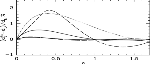
FIG. 1.: Residuals from three fitting expansions to a given model (the periodic potential given in [13]). The dashed lines are the quadratic and cubic polynomial $d_{L}$-expansion fit, the solid lines are the linear and quadratic $w$-expansion fit and the dotted line the fit according to Eqn. 3.

The $w$-expansion parameters also have an intuitive meaning in their own right. Given the uncertainty regarding causes of cosmic acceleration, it might be reasonable to simply think of the $w_{i}$’s as the fundamental parameters for now. They tell us something relatively straightforward about the nature of the dark energy. The same cannot be said of the $c_{i}$ of [9] or the $\alpha,\beta$ and $\gamma$ of [10]. We are fortunate that the twin criteria of intuitive interpretation of parameters and good fits to published models point to the same choice of fitting functions. It is worth noting however that we have not proven that the $w$-expansion provides the best possible fits to current models. It is possible that an even better choice could be discovered in the future.

Maor et al. [7] also favor the same $w$-expansion formalism. However we do not agree completely with their discussion of the alternative methods [9, 10]. Despite claims to the contrary in [7] all the approaches use “fitting functions”. If for example a new understanding of dark energy emerged in which the $c_{i}$ of [9] were fundamental parameters, then the $w$-expansion would provide a bad fit to those models and would be a bad choice for the fitting functions (whereas $d_{L}(z)=\sum_{i=1}^{N}c_{i}z^{i}$ would be an “exact expression”).

So we have argued that the $w$-expansion offers a good means of interpreting supernova data. Now we apply this expansion to simulated future supernova datasets.

For concreteness, we assume a future dataset similar to one proposed for the SNAP satellite project[5], with SNe observed uniformly within four different redshift ranges with the following different sampling rates: In the first range from $z=0-0.2$ we assume that their are $50$ observations, in the second and largest redshift range from $z=0.2-1.2$ there are $1800$ SNe and in the two high redshift bins, $z=1.2-1.4$ and $z=1.4-1.7$, there are $50$ SNe and $15$ SNe observations respectively. The statistical error in magnitude is assumed to be $\sigma_{\rm mag}=0.15$, including both measurement error and any residual intrinsic dispersion after calibration. It is worth noting that considerations such as those raised in [12] could change this redshift-distribution strategy to further optimize the impact of the data. We construct Monte Carlo simulated datasets, first for a flat, cosmological constant model with $\Omega_{\rm m}=0.3$ and $\Omega_{\Lambda}=0.7$. Figure 2 shows an example of simulated data. The points show binned data with statistical error bars, where we combine $56$ SNe in each bin.

Figure 2 shows the magnitude difference, $\Delta m$, between several dark energy models (solid) and the Monte Carlo fiducial model, along with the simulated binned data for that model. To guide the eye we also show a grid of constant $w$ models (dotted). Note how for the supergravity model [14] (labeled “SUGRA”), adding the linear term, $w_{1}$, improves the fit considerably (as shown by the dashed line, mostly covered by the solid line), compared to the best constant fit with $w_{0}=0.74$. For the two exponential model [15] (“2EXP”) the constant fit seems already sufficient. The line labeled “TOY” corresponds to a toy model with $w_{0}=-0.6$ and $w_{1}=-0.8$, which is not well represented by a constant fit. All the models have $\Omega_{m}=0.3$.

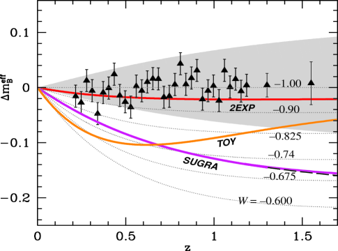
FIG. 2.: Simulated binned data, with solid curves from a supergravity inspired model [14] (with the best $N=1$ fit shown as a dashed line, mostly covered by the solid SUGRA line), a strongly evolving toy model with $w_{0}=-0.6$ and $w_{1}=-0.8$ (TOY), and a model involving two exponentials [15] (2EXP). A range of constant $w$ models is shown as a grid of lines. The shaded region corresponds to cosmological constant models with $0.25\leq\Omega_{\rm m}\leq 0.35$ and $\Omega_{\Lambda}=1-\Omega_{\rm m}$.

Figure 2 illustrates that these models can be easily

differentiated from one another by the simulated data, and that for the toy model the contribution

from $w_{1}$ looks large enough to be discriminated by the data. The targeted SNAP systematic uncertainties can be estimated by considering for example a linear drift up or down in the data (as a function of $z$) which spans one error bar height over $0<z<1.5$ (Note that a constant systematic uncertainty would not affect the results.) Further investigation is required to determine if these targets are realistic. When the targeted systematic uncertainties are taken into account the “2EXP” and $w=-1$ models can no longer be discriminated. In [6] we report more thoroughly on the models which can and cannot have $w_{1}$ differentiated from zero by such datasets. In most published models $w_{1}$ is below the level observable by supernovae alone.

We shall see below that the effect of introducing $w_{1}$ in the fit for this dataset is to substantially increase the uncertainty in $w_{0}$ (as emphasized in [7]). This is because with the additional fitting parameter there are many more ways of fitting the simulated data to good accuracy. This fact has nothing to do with the ability of the (in this case simulated) dataset to discriminate among the models shown. The ability to discriminate among the models is a fundamental property of the dataset, whereas the choice of fitting function is a matter of choosing suitable analysis techniques. As with any experimental data, for a given dataset each of the shown models is a member of a degenerate family of models that cannot be differentiated by the data. Opening up the space of fitting functions allows one to probe this degeneracy. Furthermore, we show below how realistic improvements in our independent knowledge of $\Omega_{m}$ can break this degeneracy to an interesting degree.

Figure 3 shows joint likelihood contours in the $\Omega_{m}-w_{0}$ plane for the simulated data, when these are the only parameters used to fit the data. We show also the shift due to a linearly drifting systematic error of $\pm 0.02\,{\rm mag}$ per 1.5 units in redshift. Clearly the data will discriminate among the three models shown.

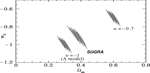
FIG. 3.: Separation of dark energy models (labeled as in Fig. 2) in the $\Omega_{\rm m}$–$w_{0}$ plane. We show $39.3\%$ ($\Delta\chi^{2}=1$, shown as solid-line contours) and 68% ($\Delta\chi^{2}=2.3$, shown as shaded contours) confidence regions which project on the axes to give marginalized $1\sigma$ and $1.5\sigma$ errors respectively. The left and right flanking contours for each model show the effects of a drifting systematic error (see text). The $w=-0.7$ model has $\Omega_{m}=0.6$, the other two models are exactly the same as their counterparts in Fig. 2. More examples are given in [6].

prior $\sigma_{\Omega_{m}}$	measurement $\sigma_{\rm mag}$	$\sigma_{w_{0}}$	$\sigma_{w_{1}}$
No ${\Omega_{m}}$ prior; $w_{1}=0$	0.15	0.06
0.15	0.15	0.15	0.6
0.05	0.15	0.06	0.2
”	0.09	0.05	0.12
0.04	0.15	0.05	0.16
0     (fixed ${\Omega_{m}}$)	0.15	0.03	0.12

TABLE I.: Statistical measurement uncertainties on $w_{0}$ (i.e., $w_{\rm today}$) and $w_{1}$, given supernova magnitude measurement uncertainty, $\sigma_{\rm mag}$, and a range of uncertainties, $\sigma_{\Omega_{m}}$, in the independent prior knowledge of $\Omega_{m}$. (As in Fig. 4, the supergravity model is used here as the example, but the other models give comparable results.) The systematic uncertainties are 0.01 in $w_{0}$ and 0.10 in $w_{1}$.

We now analyze the same simulated data using a fitting function that includes $w_{1}$. For this analysis (results shown in Table 1 and Figure 4), we consider different possible states of prior information about the value of $\Omega_{m}$, ranging from relatively poorly known ($\sigma_{\Omega_{m}}\approx 0.15$), roughly the case today, to well determined ($\sigma_{\Omega_{m}}\approx 0.04$), a possible goal within the next decade. We show in [6] that the systematic errors lead to roughly the same contribution as the statistical errors for the case of a perfectly constrained $\sigma_{\Omega_{m}}=0.0$. We conclude from Fig. 4 and Table 1 that expanding the fitting function to include $w_{1}$ will become useful when the value of $\Omega_{m}$ is better constrained than it is today. This result adds to the case for producing an independent determination of $\Omega_{m}$.

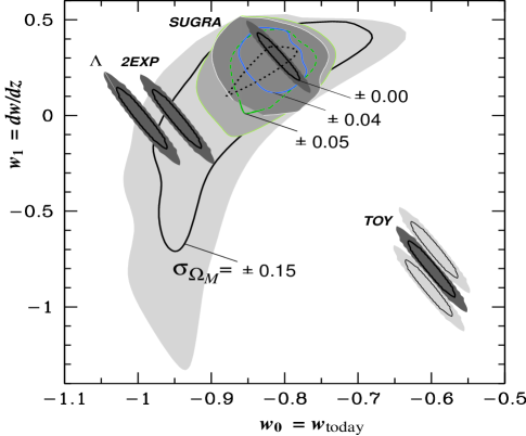
FIG. 4.: Separation of dark energy models (labeled as in Fig. 2) in the $w_{0}$–$w_{1}$ plane. The shaded regions are $39.3\%$ joint probabilities for the different $\Omega_{\rm m}$ priors and the dashed and solid lines the corresponding $68\%$ probabilities. For the example of the supergravity (SUGRA) model, a range of increasingly larger contours represents the result using prior knowledge on $\Omega_{m}$ with increasingly poorer uncertainty, $\sigma_{\Omega_{m}}$. The black dotted curve corresponds to the projected-1$\sigma$ error contour obtained for more optimistic dataset specifications ($\sigma_{\rm mag}=0.09$; see text) with a prior of $0.25\leq\Omega_{m}\leq 0.35$. For the example of the TOY model, flanking contours show the effects of a drifting systematic error (see text).

It may be possible to reduce the statistical uncertainties even further, by increasing the sample size and/or by improving the intrinsic luminosity calibration for each supernova. Figure 4 also shows the smaller likelihood region (dotted ellipse) which one gets when taking $\sigma_{\rm mag}=0.09$ and doubling the number of supernovae in each bin. This means (see Table 1) that the $1\sigma$ statistical error on $w_{1}$ improves from $\sigma_{w_{1}}=0.6$ for the current constraints on $\Omega_{m}$ (solid line in Fig.4), to $\sigma_{w_{1}}=0.2$ for future $\Omega_{m}$ constraints (dashed line), to very tight constraints of $\sigma_{w_{1}}=0.12$ for the “improved” scenario, with twice as many more-tightly-calibrated supernovae and $\sigma_{\rm mag}=0.09$ (dotted line).

Figure 4 is similar to Fig. 2 from [7]. (To compare actual numbers for predicted uncertainties, note that Maor et al. quote the full-width range of 95%-confidence contours, i.e. four times a 1$\sigma$ uncertainty. Also, our different contour shapes are due to our choice of a Gaussian probability distribution for $\Omega_{m}$ vs. their tophat distribution.) Maor et al. emphasize the uncertainties that emerge when the fitting function is expanded to include $w_{0}$ and $w_{1}$ given our current knowledge of $\Omega_{m}$. We disagree with this emphasis and focus instead on the great impact a SNAP-type experiment will have. Even if our determination of $\Omega_{m}$ were not to improve over the next decade, SNAP-class datasets would still be powerful discriminators among models. For example, such a dataset could easily discriminate between $w=-1$ (a cosmological constant) as the source of cosmic acceleration and several interesting quintessence models (such as SUGRA or others discussed in [6]). A result either way would have profound

implications. Furthermore, significant improvements on the determination of $\Omega_{m}$ are expected over the next decade and we have shown how sufficient improvements would allow the extra fitting parameter $w_{1}$ to become an “observable” and help to further differentiate theories [16].

We have investigated different analysis methods for supernova datasets, and used our preferred method to explore the prospects of further supernova searches. It is clear that a dataset of the sort proposed with SNAP [5] presents an exciting opportunity to constrain theories of cosmic acceleration.

ACKNOWLEDGMENTS: We thank S. Perlmutter for extensive discussions and in particular for emphasizing the importance of the improving knowledge of $\Omega_{m}$; D. Huterer, A. Lewin, P. Steinhardt and M. Turner for helpful conversations; and

P. Astier for comparing our results with his independent calculations. We were supported by DOE grant DE-FG03-91ER40674 and U.C. Davis.

REFERENCES

- [1] N. Bahcall, et al. Science 284, 1481, (1999).
- [2] S. Perlmutter et al., Ap. J. 483, 565 (1997).
- [3] A. Riess et al., Astron. J 116, 1009 (1998).
- [4] S. Perlmutter et al., Ap. J. 517, 565 (1999).
- [5] snap.lbl.gov
- [6] J. Weller and A. Albrecht in preparation
- [7] I. Maor et al.astro-ph/0007297
- [8] S. Perlmutter, M. S. Turner and M. White, Phys. Rev. Lett. 83, 670 (1999).
- [9] D. Huterer and M. S. Turner, Phys. Rev. D60, 081301 (1999).
- [10] T. D. Saini et al., astro-ph/9910231.
- [11] T. Chiba and T. Nakamura astro-ph/0008175
- [12] D. Huterer, M. Turner astro-ph/0006419 To appear in Proceedings of ”Sources and Detection of Dark Matter/Energy in the Universe”, Marina Del Rey, Feb. 2000
- [13] S. Dodelson,et al. astro-ph/0002360
- [14] Ph. Brax and J. Martin, Phys. Lett. B 468, 40 (1999).
- [15] T. Barreiro et al. Phys. Rev. D 61 127301 (2000)
- [16] We have assumed a completely independent measurement of . Cross-correlations will reduce this effect as discussed in Huey et al. PRD 59 073005 (1999); Wang and Steinhardt Ap. J. 508 483 (1998)