Can luminosity distance measurements probe the equation of state of dark energy

Abstract

Distance measurements to Type Ia supernovae (SNe Ia) at cosmological distances indicate that the Universe is accelerating and that a large fraction of the critical energy density exists in a component with negative pressure. Various hypotheses on the nature of this “dark energy” can be tested via their prediction for the equation of state of this component. If the dark energy is due to a scalar field, its equation of state will in general vary with time and is related to the potential of the field. We review the intrinsic degeneracies of luminosity distance measurements and compute the expected accuracies that can be obtained for the equation of state parameter from a realistic high statistic SNe Ia experiment.

1 Introduction

There is now strong evidence that the Universe is flat and that matter only amounts to about 1/3 of the critical energy, the remaining 2/3 exhibiting a large and negative pressure. There are several candidates for this dark energy component, which can be characterised by their “equation of state”, namely the ratio $w=p/\rho$. For example the genuine Cosmological Constant has $p=-\rho$, while topological defects give $p=-\rho/3$ for strings or $p=-2\rho/3$ for domain walls. But dark energy could also be due to a possibly evolving scalar field, in which case the equation of state may vary with time (and redshift).

Because they are performed at varying redshifts, luminosity distance measurements of Type Ia supernovae can, in principle, provide estimates of this possible varying equation of state. The luminosity distance, however, exhibits strong degeneracies, that may forbid any precise determination of this equation of state, especially if one allows it to vary with redshift.

We first review the expressions involved in the calculation of the luminosity distance, and examine the main degeneracy that shows up when analysing a simulated (yet realistic) high statistics SNe Ia experiment. We then show how independent knowledge of $\,{\Omega_{\rm M}}$ will limit the effects of the degeneracy and compute the expected statistical and systematic uncertainties that can be achieved with such an experiment.

2 Basic Equations

We assume a flat universe made of 2 components : non-relativistic matter, which contributes $\,{\Omega_{\rm M}}$ to the critical density, and a single extra component $X$ described by its equation of state as a function of redshift:

$$\,{w_{\rm X}}(z)=\,{p_{\rm X}}(z)/\,{\rho_{\rm X}}(z)$$ (1)

The luminosity distance reads:

$$d_{L}(z)=(1+z)r(z)=(1+z)\int_{0}^{z}\frac{dz^{\prime}}{H(z^{\prime})}$$ (2)

where r(z) is the Robertson-Walker comoving coordinate to an object seen (via massless photons) at a redshift z. Friedman’s equation for a two component flat universe reads:

$$H^{2}(z)=H_{0}^{2}(\,{\rho_{\rm M}}(z)+\,{\rho_{\rm X}}(z))/\rho_{0}$$ (3)

where $\,{\rho_{\rm M}}$ is the matter density, $\,{\rho_{\rm X}}$ is the dark energy density, and $\rho_{0}$ is the total density today. The equation of state defines the way the component x behaves with expansion:

$$\dot{\rho}_{\rm X}=-3H(1+\,{w_{\rm X}})\,{\rho_{\rm X}}$$ (4)

Using $dz=-(1+z)Hdt$, this equation can be integrated:

$$\,{\rho_{\rm X}}(z)=\,{\rho_{\rm X}}(0)\exp{3\int_{0}^{z}dz^{\prime}\frac{1+\,{w_{\rm X}}(z^{\prime})}{1+z^{\prime}}}.$$ (5)

One may notice that $\,{w_{\rm X}}=-1$ corresponds to a constant $\,{\rho_{\rm X}}$. For the matter component, $\,{\rho_{\rm M}}$, $w=0$ which leads to $\,{\rho_{\rm M}}(z)=\,{\rho_{\rm M}}(0)(1+z)^{3}$. Since observations favour a negative $\,{w_{\rm X}}$ ([5]), $\,{\rho_{\rm M}}/\,{\rho_{\rm X}}$ very likely increases with redshift.

The luminosity distance can be written:

$$d_{L}(z)=\frac{1+z}{H_{0}}\int_{0}^{z}\frac{dz^{\prime}}{\sqrt{\,{\Omega_{\rm M}}(1+z^{\prime})^{3}+(1-\,{\Omega_{\rm M}})\,{\rho_{\rm X}}(z)/\,{\rho_{\rm X}}(0)}}$$ (6)

$\,{w_{\rm X}}(z)$ is the (unknown) function to be determined from measurements of $d_{L}$ at various redshifts. For dark energy with negative pressure ($\,{w_{\rm X}}<0$i), the higher the redshift, the higher the relative matter contribution in the above equation.

To see how the unknown $\,{w_{\rm X}}$ depends on the data $d_{L}$, one may invert Equation 6, first by deriving it with respect to z:

$$\log{\frac{{r^{\prime}}^{-2}-H_{0}^{2}\,{\Omega_{\rm M}}(1+z)^{3}}{H_{0}^{2}(1-\,{\Omega_{\rm M}})}}=3\int_{0}^{z}\frac{1+\,{w_{\rm X}}(z^{\prime})}{1+z^{\prime}},$$ (7)

where $r(z)=d_{L}(z)/(1+z)$, and $r^{\prime}=dr/dz$. Deriving once again yields:

$$1+\,{w_{\rm X}}(z)=\frac{1+z}{3}\frac{3H_{0}^{2}\,{\Omega_{\rm M}}(1+z)^{2}+2r^{\prime\prime}/{r^{\prime}}^{3}}{H_{0}^{2}\,{\Omega_{\rm M}}(1+z)^{3}-{r^{\prime}}^{-2}}$$ (8)

So, $\,{w_{\rm X}}$ is related to the first and second derivatives of the distance in a highly non-linear way. Furthermore, the terms in the sums composing the numerator and denominator of Equation 8 are of comparable size and opposite sign: they typically differ by 30 % at a redshift of 1. As a consequence, small variations of the derivatives of r will result in large variations of $\,{w_{\rm X}}$. This is shown the other way around in [1], through striking plots.

Several papers recently addressed the problem of reconstructing $\,{w_{\rm X}}$ (or equivalently the potential of a scalar field) from luminosity distance measurements. Some conclude that it is hopeless given expected uncertainties of large statistics SNe Ia measurements [1], others provide reasonably accurate estimations of $\,{w_{\rm X}}(z)$, either based on Monte-Carlo experiments [2], or even on available SNe Ia data [4]. Before attempting to clarify what causes these fundamental differences, we will warn the reader about a potential misconception that may arise from Equation 8: both its numerator and denominator are insensitive to $H_{0}$ because r scales as $H_{0}^{-1}$. Hence w depends on $\,{\Omega_{\rm M}}$ and not on $\,{\Omega_{\rm M}}H_{0}^{2}$, nor on $H_{0}$.

3 Measurements and uncertainties

Type Ia supernovae, have been used to constraint cosmological parameters [5, 6]. Using the light curve width-peak brightness empirical relation, the intrinsic dispersion of peak brightness of SNe Ia was found to be about 0.15 magnitude. A measurement with an total error of 0.2 magnitude is already possible (it is the best resolution obtained in [5]), and we will assume conservatively this value as a standard error. It translates into relative uncertainties of measured luminosity distances of 10 %, which makes the current redshift measurement uncertainty totally negligible. For the proposed SNAP space mission [7], the accessible redshift range is limited to 1.7, due mainly to the overwhelming integration times required to reach the expected signal to noise. There is also a limitation on the low redshift side due to the large area that has to be covered to discover a sufficient number of low redshift supernovae. Minimising systematic errors dictates that the whole sample is observed using the same apparatus. We will therefore consider as a conservative baseline that 2000 SNe Ia with redshifts in the range $[0.2,1.4]$ can be efficiently observed and see how well we can reconstruct $\,{w_{\rm X}}(z)$.

If we have a dataset of SNe Ia with redshifts ${z_{i},i=1..N}$, we may compute least squares estimates of the cosmological parameters by minimising:

$$\chi^{2}=\sum_{i=1}^{N}\frac{(d_{i}-d_{L}(z_{i},\theta))^{2}}{(pd_{i})^{2}}$$ (9)

where $d_{i}$ is the measured luminosity distance, $\theta$ is the set of cosmological parameters to estimate, $d_{L}(z_{i},\theta)$ is the expected value of the luminosity distance for the redshift $z_{i}$ and the cosmological parameters $\theta$, p is the relative error (assumed to be 0.1) on the measurement.

If one assumes that $\,{w_{\rm X}}$ is constant($\,{w_{\rm X}}=w_{0}$), $\theta$ is a 2 component vector $(\,{\Omega_{\rm M}},w_{0})$. To estimate a varying $\,{w_{\rm X}}$ without any prejudice, one may parametrise $\,{w_{\rm X}}$ as a polynomial:

$$\,{w_{\rm X}}=\sum_{i=0}^{d}w_{i}z^{i}$$ (10)

Choosing a polynomial of z or 1+z does not make any difference from the estimation point of view since there is a one-to-one mapping of the coefficients. Using this expression for $\,{w_{\rm X}}$, Equation 6 can be rewritten (for clarity we limit the polynomial to d=2):

$$d_{L}(z)=\frac{1+z}{H_{0}}\int_{0}^{z}\frac{dz^{\prime}}{\sqrt{\,{\Omega_{\rm M}}(1+z^{\prime})^{3}+(1-\,{\Omega_{\rm M}})W(z^{\prime})}}$$ (11)

where $W(z)=(1+z)^{w_{0}-w_{1}+w_{2}}\exp((w_{1}-w_{2})z+w_{2}z^{2}/2)$.

For models with varying $\,{w_{\rm X}}$, we will concentrate on estimating the 3 parameters: $(\,{\Omega_{\rm M}},w_{0},w_{1})$, which is enough to illustrate where the difficulties show up, for 3 different universes $(\,{\Omega_{\rm M}},w_{0},w_{1})$ = (0.3,-1.0,0.0), (0.3,-0.8,0.3) and (0.4,-1.0,1.0), labelled A B and C in the figures. Model A is the standard Cosmological Constant, model B is close to a quintessence model with an inverse power law potential modified by supergravity [3], and model C is a toy model with a rapidly varying w.

The (logarithmic) derivatives shown in Figure 1 determine the information that every supernova adds as a function of redshift. It is clear that higher redshifts provide more information, but this becomes less clear if one considers that several lower redshift objects can be measured in the time required for the measurement of one high redshift object. One important point to notice is that for a given model, all derivatives are very similar in shape which means that the parameter combination that a redshift probes does not vary strongly with redshift.

Figure 1: Logarithmic derivatives of the luminosity distance w.r.t $\,{\Omega_{\rm M}}$, $w_{0}$ and $w_{1}$, for the 3 models under study (see text), as a function of redshift. One may notice similar shapes of the three derivatives for every model.

To study what influences the variance (and covariance) of parameter estimates, we will restrict ourselves to the quadratic approximation of the $\chi^{2}$ which consists in linearising $d_{L}$ as a function of parameters around the chosen model. This is clearly not to be done for an actual estimation, where an accurate mapping of the actual $\chi^{2}$ values (or of the likelihood) is necessary to obtain reliable confidence contours. Within this linear approximation, the Hessian of the $\chi^{2}$ w.r.t the parameters reads:

$$\frac{1}{2}\frac{\partial^{2}\chi^{2}}{\partial\theta^{2}}=F=\sum_{i=1}^{N}h(z_{i},\theta)h^{T}(z_{i},\theta),\hskip 14.22636pt{\rm with}\hskip 14.22636pth(z_{i},\theta)=\frac{1}{pd_{L}}\frac{dd_{L}(z_{i},\theta)}{d\theta}$$ (12)

All derivatives are usually evaluated at the minimum $\chi^{2}$ (i.e. the parameter estimate). As we are studying the estimation variance as a function of parameters and dataset, we will evaluate the derivatives at the parameter value, which should be the average estimate value. Since $\theta$ is vector, h is also a vector, and F is then a matrix, called the Fisher (or information or sometimes weight) matrix. Every $hh^{T}$ term of the sum is a matrix of rank 1 that is the information on the parameters that a given supernova adds. Within this linear approximation, The covariance matrix of the estimates is just $C=F^{-1}$.

model	“C”	$\sqrt{\lambda}$	Eigenvectors
A	$\begin{matrix}0.2666&-0.9853&-0.9951\\ -0.9853&0.2826&0.9643\\ -0.9951&0.9643&2.117\\ \end{matrix}$	$\begin{matrix}0.00417\\ 0.0781\\ 2.152\\ \end{matrix}$	$\begin{matrix}0.9418&0.3274&0.07586\\ 0.3126&-0.9363&0.1598\\ -0.1233&0.1268&0.9842\\ \end{matrix}$
B	$\begin{matrix}1.1913&-0.9996&-0.9976\\ -0.999608&1.42776&0.9953\\ -0.9976&0.9953&2.290\\ \end{matrix}$	$\begin{matrix}0.0053\\ 0.125\\ 2.948\\ \end{matrix}$	$\begin{matrix}0.8516&0.5086&0.1263\\ 0.3339&-0.7123&0.6172\\ -0.4039&0.4834&0.7765\\ \end{matrix}$
C	$\begin{matrix}0.2762&-0.9964&0.6763\\ -0.9964&0.5835&-0.7339\\ 0.6763&-0.7339&0.26285\\ \end{matrix}$	$\begin{matrix}0.0060\\ 0.174\\ 0.675\\ \end{matrix}$	$\begin{matrix}0.8840&0.4538&0.1111\\ -0.2333&0.222&0.9465\\ -0.4048&0.8627&-0.3028\\ \end{matrix}$

Table 1: Covariance matrix of the estimates for our 3 models (where diagonal elements are the rms errors and off-diagonal elements are the correlation coefficients). Second column gives the square root of eigenvalues, the third gives the corresponding eigenvectors. One may notice that the last eigenvector totally dominates the error budget. Especially for model B, the errors induced by the degeneracy forbid any independent measurement of the parameters.

Table 1 gives C and its eigenvalues and eigenvectors within the linear approximation for our 3 universes, and for 2000 uniformly spread supernovae over the redshift range, the distance to each of them measured with a 10 % accuracy (0.2 mag): for model B (the worst case), the ratio of major to minor axis of the error ellipsoid is more than 500, which means that the parameter combination corresponding to the last eigenvector is almost unmeasured.

The dataset as proposed does not allow to estimate jointly $\,{\Omega_{\rm M}}$, $w_{0}$ and $w_{1}$ with a decent precision. However, one should notice that the problem is very different if $\,{\Omega_{\rm M}}$ is frozen, in which case the errors on $w_{0}$ and $w_{1}$ go down by more than one order of magnitude. In [2, 4], $\,{\Omega_{\rm M}}$ is fixed, unlike in [1] where $\,{\Omega_{\rm M}}$ is estimated and marginalized over. This explains partly why these papers reach different conclusions.

The reason for this large degeneracy can be found by expanding in powers of z the expression for $H^{2}$ under the square root in Equation 11 (which is probed observationally through $(dr/dz)^{-1/2}$):

$$\frac{H^{2}(z)}{H_{0}^{2}}=1+3(1+\,{\Omega_{\rm X}}w_{0})z+3/2(2+5\,{\Omega_{\rm X}}w_{0}+\,{\Omega_{\rm X}}w_{1}+3\,{\Omega_{\rm X}}w_{0}^{2})z^{2}+o(z^{3})$$ (13)

where $\,{\Omega_{\rm X}}=1-\,{\Omega_{\rm M}}$.

Consider for a while $w_{1}=0$: at first order in z, only $\,{\Omega_{\rm X}}w_{0}$ is determined (as shown by the shape of the confidence contours in the $(\,{\Omega_{\rm M}},w_{0})$ plane shown in [5]), the second order fixes $w_{0}$ through $\,{\Omega_{\rm X}}w_{0}^{2}$, which is rather weak. $(\,{\Omega_{\rm X}}w_{0},\,{\Omega_{\rm X}}w_{0}^{2})$ are much closer to observable that $(\,{\Omega_{\rm M}},w_{0})$, but $\,{\Omega_{\rm X}}w_{0}^{2}$ really lacks physical sense. The scheme is the same for $w_{1}$: it enters through $\,{\Omega_{\rm X}}w_{1}$ at second and third order and through $\,{\Omega_{\rm X}}w_{0}w_{1}$ at third order. As a consequence the parametrisation $(\,{\Omega_{\rm M}},\,{\Omega_{\rm X}}w_{0},\,{\Omega_{\rm X}}w_{1})$ is not much less degenerate than the one considered here.

Obviously, the main degeneracy goes away when fixing $\,{\Omega_{\rm M}}$. Before studying how the uncertainties on $\,{\Omega_{\rm M}}$ affect w, we will evaluate the effect of optimising the redshift distribution of the dataset.

4 Optimising the redshift distribution of the dataset

To optimise the redshift distribution of the dataset, we first study the effect on the largest eigenvalue of C, of adding to the total sample a small number of supernovae (e.g. 40) in a given redshits bin. Figure 2 shows how this quantity evolves as a function of the redshift in which the 40 supernovae were added. Although no dramatic change is seen (errors scale as the plotted values), Figure 2 shows that a small subsample collected at much higher redshift would reduce the errors more efficiently than collecting more events in the original redshift interval.

Figure 2: value of the square root of the largest eigenvalue of C as a function of the redshift where one adds 40 supernovae to the sample.

One may want to be more radical, i.e. really optimise the redshift distribution within the redshift range in order to minimise this largest eigenvalue, keeping constant the total number of supernovae. This does not yield the same result as minimising the determinant of C as done in [9] where the optimal determinant is obtained at the cost of an even higher largest eigenvalue. However, as for the minimum determinant, the optimum is reached for a redshift distribution consisting in 3 delta functions, that are given in Table 2. The improvement with respect to a flat distribution is not large enough to consider seriously such an extreme option, which has very severe drawbacks. Nevertheless, a moderate optimisation of the redshift distribution would be worth doing since it would lead to a gain in resolution.

model	“C”	z1 z2 z3	fractions
A	$\begin{matrix}0.1714&-0.9720&-0.989\\ -0.972&0.1941&0.9295\\ -0.989&0.9295&1.341\\ \end{matrix}$	$\begin{matrix}0.20\\ 0.82\\ 1.40\\ \end{matrix}$	$\begin{matrix}0.40\\ 0.40\\ 0.20\\ \end{matrix}$
B	$\begin{matrix}0.7798&-0.9989&-0.9944\\ -0.9989&0.9393&0.9887\\ -0.9944&0.9887&1.478\\ \end{matrix}$	$\begin{matrix}0.20\\ 0.91\\ 1.40\\ \end{matrix}$	$\begin{matrix}0.34\\ 0.41\\ 0.25\\ \end{matrix}$
C	$\begin{matrix}0.1828&-0.9918&0.3483\\ -0.9918&0.3715&-0.4583\\ 0.3483&-0.4583&0.1957\\ \end{matrix}$	$\begin{matrix}0.20\\ 0.86\\ 1.40\\ \end{matrix}$	$\begin{matrix}0.50\\ 0.36\\ 0.14\\ \end{matrix}$

Table 2: Result of optimisation of the redshift distribution to reduce the largest eigenvalue of C (where C is given the same way as in Table 1). The 3 optimal distributions are rather similar.

5 Expected accuracy on $w_{0}$ and $w_{1}$ imposing an $\,{\Omega_{\rm M}}$ prior

We computed in the Bayesian approach the $w_{0}$,$w_{1}$ joint confidence contours, by marginalizing the estimate probability distribution over $\,{\Omega_{\rm M}}$ with a Gaussian prior, without recourse to the linear approximation, We used a Gaussian prior with $\sigma=0.05$, which is 2 to 3 times better than nowadays precision from large scale structures, and other methods. The results are shown in Figure 2. Despite our conservative inputs, model A and model B can be separated at more than 95 % CL, whatever is the true one. Model B can be separated from domain walls ($(w_{0},w_{1})=(-2/3,0)$) with the same accuracy.

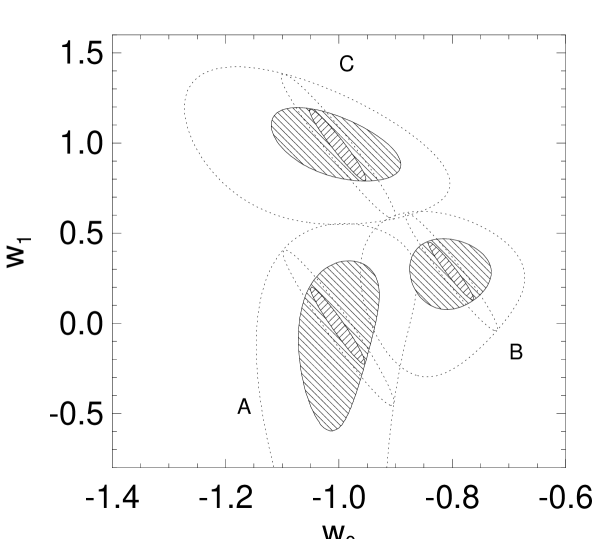
Figure 3: 1 and 2 $\sigma$ (39% filled areas,86% dotted lines) confidence contours for ($w_{0}$,$w_{1}$) with a Gaussian prior $\sigma_{\,{\Omega_{\rm M}}}=0.05$ (large contours), and with an infinite precision (small elongated contours). For model A, the 2 $\sigma$ contour escapes in an unphysical region.

It is interesting to come back again to the linear approximation to study how estimated errors scale with the (external) $\,{\Omega_{\rm M}}$ uncertainty, and the (internal) precision of the luminosity distance measurements. Adding a prior is adding a $((\,{\Omega_{\rm M}}-\,{\Omega_{\rm M}}^{\prime})/\sigma)^{2}$ to the $\chi^{2}$, where $\,{\Omega_{\rm M}}^{\prime}$ is the prior value, and $\,{\Omega_{\rm M}}$ remains the parameter to be estimated. The Fisher and covariance matrix become:

$$F^{\prime}=F+\frac{pp^{T}}{\sigma^{2}},\hskip 28.45274ptC^{\prime}=C-\frac{(Cp)(Cp)^{T}}{\sigma^{2}+p^{T}Cp}$$ (14)

where $C=F^{-1}$ and $p=(1,0,0)$ is the (unit) vector describing the prior (here it only concerns $\,{\Omega_{\rm M}}$) and $\sigma$ is its standard error. The a posteriori variance of e.g. $w_{1}$ (after application of the prior) reads:

$$V(w_{1}) = C^{\prime}_{33}=C_{33}-\frac{(C_{31})^{2}}{\sigma^{2}+C_{11}}=C_{33}(1-\frac{\rho_{13}^{2}}{\sigma^{2}/C_{11}+1})$$ (15)

$$\simeq C_{33}(1-\rho^{2}_{13}+\rho^{2}_{13}\sigma^{2}/C_{11})$$

where the last approximation holds for $\sigma^{2}<<C_{11}$ (which is already the case with nowadays precision on $\,{\Omega_{\rm M}}$). $V(w_{1})$ scales with $\sigma^{2}$ for large $\sigma$, and with $C_{33}$ for smaller ones. When $\sigma=C_{11}(1-\rho_{13}^{2})/\rho_{13}^{2}$, $V(w_{1})$ is twice its minimum value ($\sigma=0$). This happens for $\sigma=0.03,0.08,0.44$ for models A,B and C respectively. Doing the same exercise for $w_{0}$ yields $\sigma=0.05,0.03,0.02$. With $\sigma=0.05$ and our assumptions for the experimental precision, the result quality would benefit both from a smaller $\sigma$ and from a better luminosity distance measurement.

For an infinitely well defined $\,{\Omega_{\rm M}}$, we face a second “degeneracy” demonstrated by the elongated shape of the error contours. The orientation of the major axis defines a z ($z_{min}$) for which $Var(w_{0}+w_{1}z)$ is minimal, $z_{min}\simeq$ 0.2 to 0.3. Models with similar $\,{w_{\rm X}}(z_{min})$ but different $w_{1}$ (within $\sim$ 0.3 in our assumptions), will be indistinguishable. This is shown by Figure 1 of [1] where luminosity distances for different $w_{X}$ having similar $w_{X}(z=0.3)$ are shown to have the same luminosity distance behaviour.

6 Influence of systematic errors

The overall scale of luminosity distances (deduced from fluxes) depends on $LH_{0}^{2}$, where L is the absolute luminosity of the candle. So distortions that bias the cosmological parameters are the ones that distort the shape of $d_{L}$. At lowest order in z, we may model:

$$d_{L}^{measured}=d_{L}^{true}(1+\alpha z),\hskip 28.45274pt$$ (16)

where $\alpha$ (hopefully small) accounts for example for the drift of photometric calibration of supernovae across the redshift range, an unknown evolution of supernovae, or light absorption in the intergalactic medium uniformly over the spectral range. The SNAP mission has been designed to reduce these effects as much as possible, and targets a precision of 0.02 mag over the redshift range $z<1.7$ which corresponds to $|\alpha|<0.006$.

We computed the parameter biases for our 3 models, with $\sigma_{\,{\Omega_{\rm M}}}=0.05$ and $\alpha=0.01$, and found negligible shifts for $\,{\Omega_{\rm M}}$ (as expected), and biases for $(w_{0},w_{1})$ of (0,-0.19), (-0.01, 0.10) and (-0.02,-0.12) for models A,B and C. These systematic biases are all below the statistical uncertainty, and do not change significantly for $\sigma_{\,{\Omega_{\rm M}}}$ = 0.1 or 0.025.

7 Conclusions

With conservative hypotheses for the expected performances of a future high statistics SNe Ia experiment such as the proposed SNAP mission, we find that the equation of state parameter of the dark energy can be measured provided an accurate value of $\,{\Omega_{\rm M}}$ is used as a prior. Detailed study of Type Ia supernovae such as with the planned nearby supernova factory project [8] could result in further reducing the peak-brightness intrinsic dispersion which directly affects the precision on the equation of state parameter. In addition, independent gain of precision can be achieved by (moderately) optimising the redshift distribution of the dataset. Finally, it is interesting to note that the required precision on $\,{\Omega_{\rm M}}$ could come from the SNAP mission itself, using large scale weak lensing which is sensitive to $\,{\Omega_{\rm M}}$ almost independently of dark energy. In [10], a ground based moderately deep weak lensing survey of 5x5 degrees is estimated to measure $\,{\Omega_{\rm M}}$ to 10% (for $\,{\Omega_{\rm M}}$ around 0.3), reaching 5% for a 10x10 degrees survey.

References

- [1] I. Maor, R. Brustein and P. J. Steinhardt, astro-ph 0007297
- [2] D. Huterer and M. S. Turner, Phys Rev, D60 081301 (1998)
- [3] Ph. Brax, J. Martin, Phys Lett. B468 (1999) 40.
- [4] T. D. Saini et al, astro-ph 9910231.
- [5] S. Perlmutter, et al Astrophys. J. 517, 565 (1999)
- [6] A. Riess, et al, Astron. J., 116, 1009 (1998).
- [7] http://snap.lbl.gov
- [8] http://snfactory.lbl.gov
- [9] D. Huterer and M. S. Turner, astro-ph 0006419.
- [10] L. van Waerbeke, F. Bernardeau and Y. Mellier, Astron. Astrophys. 342(1999) 15-33