Study of the ammonia emission in the NGC 6334 region

Abstract

The region centered in the NGC 6334 I(N) radio continuum source was surveyed in an extension of 6′ in right ascension and 12′ in declination, in the NH₃(J,K) = (1,1) transition, using the Itapetinga radio telescope. The spectra show non-LTE behavior, and gradients of velocity and line-width were detected along the region. A detailed analysis of the spectra showed that the surveyed region is composed of at least three overlapped sources related to regions that are in different stages of star formation: NGC 6334 I, associated with an already known molecular bipolar outflow, NGC 6334 I(N)w, the brightest ammonia source, coincidental with the continuum source NGC 6334 I(N), and NGC 6334 I(N)e, weaker, more extended and probably less evolved than the others. The physical parameters of the last two sources were calculated in non-LTE conditions, assuming that their spectra are the superposition of the narrow line spectra produced by small dense clumps. The H₂ density, NH₃ column density, kinetic temperature, diameter and mass of the clumps were found to be very similar in the two regions, but the density of clumps is lower in the probably less evolved source NGC 6334 I(N)e. Differences between the physical parameters derived assuming LTE and non-LTE conditions are also discussed in this work.

1 Introduction

The NGC 6334 region, located at a distance of 1.74 kpc from the Sun (Neckel nec78 (1978)), is a complex of radio and infrared sources (Shaver & Goss shgo70 (1970); Haynes et al. hay78 (1978); McBreen et al. mcb79 (1979)). One of its components, NGC 6334 I(N), is also the strongest source in the NH₃(J,K) = (1,1) transition (e.g., Schwartz et al. sch78 (1978)). It is also a strong continuum source at 400, 1000 and 1300 $\mu$m (Cheung et al. che78 (1978); Gezari gez82 (1982); Loughran et al. lou86 (1986)) but it is below the detection limit at wavelengths smaller than 137 $\mu$m. It has an H₂O maser source, CH₃OH masers (Moran & Rodríguez moro80 (1980); Kogan & Slysh kosl98 (1998); Walsh et al. wal98 (1998)), six reddened sources at the JHK bands (Tapia et al. tap96 (1996)), a bipolar molecular outflow in SiO and eight knots of H₂ emission (Megeath & Tieftrunk meti99 (1999)). However, no H ii region associated to this source was detected.

The source NGC6334 I, located approximately 2′ south of NGC 6334 I(N), has H₂O, OH and CH₃OH masers (Moran & Rodríguez moro80 (1980); Gaume & Mutel gamu87 (1987); Forster & Caswell foca89 (1989); Menten & Batrla meba89 (1989)), an ultra-compact H ii region (Rodríguez et al. rod82 (1982); DePree et al. dep95 (1995)) and a cluster of stars detected at the JHK bands (Tapia et al. tap96 (1996)). It was studied with high angular resolution in the NH₃(J,K) = (1,1) transition by Jackson et al. (jac88 (1988)) (hereafter, JHH88), who interpreted the observed structure as a circumstellar molecular disk rotating around a 30 $M_{\sun}$ O star. On the other hand, CO and H₂ observations suggest that the structure arises from a molecular bipolar outflow (Bachiller & Cernicharo bace90 (1990); Persi et al. per96 (1996)). Due to these characteristics, it is probable that this region is in a more advanced stage of stellar formation than NGC 6334 I(N).

Both regions have been studied in several transitions of ¹²CO, ¹³CO and CS (Kraemer & Jackson krja99 (1999)), the meta-stable transitions of the ammonia molecule, including NH₃(J,K) = (1,1), (2,2), (3,3) and (6,6) [e.g., Schwartz et al. sch78 (1978); Forster et al. for87 (1987); Vilas-Boas et al. vil88 (1988); Jackson et al. jac88 (1988); Kuiper et al. kui95 (1995); Kraemer & Jackson krja95 (1995), krja99 (1999)], and the non-meta-stable transition NH₃(J,K) = (2,1) (Kuiper et al. kui95 (1995)). The physical parameters of these regions were always derived from the NH₃(J,K) = (1,1) and (2,2) observations, assuming LTE conditions. In fact, the intensity anomalies in the nuclear quadrupole hyperfine structure of the NH₃(J,K) = (1,1) spectrum are usually neglected, although they are observed in many warm molecular clouds (Stutzki et al. stu82 (1982); Batrla et al. bat83 (1983); Stutzki et al. stu84 (1984)).

Matsakis et al. (mat77 (1977)) interpreted the anomalous spectrum as the consequence of non-thermal population in the hyperfine states, induced by selective trapping in the hyperfine transitions of NH₃(J,K) = (2,1) $\rightarrow$ (1,1). This effect is relevant only when the width of the hyperfine lines lie between 0.3 and 0.6 km s^-1. Due to this restriction, they assumed that the molecular cloud is formed by clumps, each one producing a narrow line spectrum, so that the observed spectrum would be the superposition of individual clump spectra. Based on this model, Stutzki & Winnewisser (stwi85 (1985)) (hereafter, SW85) elaborated a numerical algorithm to calculate the brightness temperature ratios between the hyperfine satellites and the main line in the NH₃(J,K) = (1,1) spectrum, and also the brightness temperature ratio between the (2,2) to the (1,1) main lines, as a function of the NH₃ column density, H₂ density and kinetic temperature of each clump.

Gaume et al. (gau96 (1996)) questioned this model, based on observations of the NH₃(J,K) = (1,1) absorption spectra towards the continuum source DR21. Their argument was based on an anti-correlation in the degree of LTE departure of the inner and outer hyperfine components in different regions of the cloud. They proposed instead, inflows and outflows of matter to explain the observations, but did not present any quantitative calculation to support their claim.

In this work, we used our high quality observations of the NGC 6334 region in the NH₃(J,K) = (1,1) transition, which allowed the precise determination of the intensity anomalies in the hyperfine structure, to obtain with good reliability its physical parameters assuming non-LTE conditions. The data allowed us also to separate in the spectra the contribution of at least three different sources: NGC 6334 I, NGC 6334 I(N)w and NGC 6334 I(N)e.

2 Observations

The observations were made during July 1996 using the 13.7 m radome enclosed radio telescope of the Itapetinga Radio Observatory. The receiver front-end consisted of a circularly polarized corrugated horn connected to a cooled HEMPT. An acusto-optical spectrometer was used in the back-end, with spectral resolution and total bandwidth of 70 kHz and 41 MHz respectively. The total system temperature was about 200 K. The angular resolution of the radio telescope at the frequency of NH₃(J,K) = (1,1) transition was 4.2′. The observations were made using the ON-OFF total-power technique, switching between positions every 20 s with amplitude of 20′ in azimuth, enough to guarantee that there was no source in the OFF position. The effective integration time of each observation was 210 s. A 15 K noise source and a room temperature load were used in the calibration to obtain the gain and to correct for atmospheric attenuation (Abraham & Kokubun abko92 (1992)). The continuum point source Virgo A was used as a primary calibrator. The NGC 6334 region was mapped in the NH₃(J,K) = (1,1) transition, covering 6′ in right ascension and 12′ in declination, with a spacing of 2′. The central position of the map, with equatorial coordinates $\alpha(1950)=17\rm^{h}17\rm^{m}32\rm^{s}$ and $\delta(1950)=-35\degr 42\arcmin$, was observed several times during the mapping period and was used as secondary calibrator. This position was also observed in the NH₃(J,K) = (2,2) transition.

A polynomial baseline was subtracted from the observations and the five Gaussian functions were fitted to the hyperfine NH₃(J,K) = (1,1) spectra. The velocity separation between the Gaussians was fixed and the line-width of the hyperfine satellites constrained to be equal to the main line. This last assumption is well justified, since the optical depth of the main line is small ($\tau\sim 1.4$).

The results from the observations are presented in Table 1. The first column shows the position in the map relative to the central coordinate, columns 2-6 exhibit the antenna temperature of each transition corrected for atmospheric attenuation, columns 7 and 8 the velocity and line-width of the main line and the last column the number of observations made in each position. The NH₃(J,K) = (1,1) spectra of some points of special interest, as well as the NH₃(J,K) = (2,2) spectrum of the central position are shown in Figure 1.

Table 1: Parameters obtained from the Gaussian fitting for each position in the map.

($\Delta\alpha,\Delta\delta$)a	TA(F=1$\rightarrow$0)	TA(F=1$\rightarrow$2)	TA($\Delta$F=0)	TA(F=2$\rightarrow$1)	TA(F=0$\rightarrow$1)	vLSRb	$\Delta$vFWHM	#c
(arcmin)	(K)	(K)	(K)	(K)	(K)	(km s-1)	(km s-1)
(-2,-2)	0.17 $\pm$ 0.04	0.27 $\pm$ 0.04	0.67 $\pm$ 0.04	0.24 $\pm$ 0.04	0.26 $\pm$ 0.04	-5.09 $\pm$ 0.12	6.00 $\pm$ 0.13	4
(-2,0)	0.15 $\pm$ 0.03	0.24 $\pm$ 0.03	0.54 $\pm$ 0.03	0.21 $\pm$ 0.03	0.20 $\pm$ 0.03	-4.40 $\pm$ 0.12	4.28 $\pm$ 0.12	4
(-2,2)	0.09 $\pm$ 0.03	0.13 $\pm$ 0.03	0.43 $\pm$ 0.03	0.15 $\pm$ 0.03	0.14 $\pm$ 0.03	-3.82 $\pm$ 0.12	3.06 $\pm$ 0.13	3
(0,-4)	0.15 $\pm$ 0.04	0.23 $\pm$ 0.04	0.39 $\pm$ 0.04	0.12 $\pm$ 0.04	0.11 $\pm$ 0.04	-4.66 $\pm$ 0.12	6.29 $\pm$ 0.12	4
(0,-2)	0.30 $\pm$ 0.03	0.43 $\pm$ 0.03	0.86 $\pm$ 0.03	0.33 $\pm$ 0.03	0.32 $\pm$ 0.03	-4.98 $\pm$ 0.12	5.57 $\pm$ 0.12	2
(0,0)	0.41 $\pm$ 0.01	0.62 $\pm$ 0.01	1.41 $\pm$ 0.01	0.53 $\pm$ 0.01	0.52 $\pm$ 0.01	-4.66 $\pm$ 0.12	4.26 $\pm$ 0.12	19
(0,2)	0.30 $\pm$ 0.04	0.51 $\pm$ 0.04	1.05 $\pm$ 0.04	0.42 $\pm$ 0.04	0.43 $\pm$ 0.04	-4.21 $\pm$ 0.12	4.06 $\pm$ 0.12	2
(0,4)	0.15 $\pm$ 0.03	0.24 $\pm$ 0.03	0.62 $\pm$ 0.03	0.17 $\pm$ 0.03	0.29 $\pm$ 0.03	-3.36 $\pm$ 0.12	3.11 $\pm$ 0.12	4
(2,-4)	0.10 $\pm$ 0.04	0.22 $\pm$ 0.04	0.44 $\pm$ 0.04	0.21 $\pm$ 0.04	0.21 $\pm$ 0.04	-5.98 $\pm$ 0.12	5.37 $\pm$ 0.12	2
(2,-2)	0.27 $\pm$ 0.04	0.39 $\pm$ 0.04	0.86 $\pm$ 0.04	0.34 $\pm$ 0.04	0.34 $\pm$ 0.04	-5.29 $\pm$ 0.12	4.57 $\pm$ 0.12	2
(2,0)	0.38 $\pm$ 0.02	0.54 $\pm$ 0.02	1.28 $\pm$ 0.02	0.47 $\pm$ 0.02	0.48 $\pm$ 0.02	-4.74 $\pm$ 0.12	4.09 $\pm$ 0.12	6
(2,2)	0.34 $\pm$ 0.06	0.32 $\pm$ 0.06	1.06 $\pm$ 0.06	0.47 $\pm$ 0.06	0.43 $\pm$ 0.06	-4.43 $\pm$ 0.12	4.21 $\pm$ 0.13	1
(2,4)	0.16 $\pm$ 0.03	0.28 $\pm$ 0.03	0.59 $\pm$ 0.03	0.25 $\pm$ 0.03	0.23 $\pm$ 0.03	-3.71 $\pm$ 0.12	3.53 $\pm$ 0.13	3
(2,6)	0.13 $\pm$ 0.03	0.18 $\pm$ 0.03	0.38 $\pm$ 0.03	0.19 $\pm$ 0.03	0.16 $\pm$ 0.03	-3.07 $\pm$ 0.12	2.24 $\pm$ 0.13	4
(2,8)	0.10 $\pm$ 0.04	0.10 $\pm$ 0.04	0.25 $\pm$ 0.04	0.07 $\pm$ 0.04	0.10 $\pm$ 0.04	-3.42 $\pm$ 0.12	4.10 $\pm$ 0.12	4
(4,-2)	0.04 $\pm$ 0.03	0.07 $\pm$ 0.03	0.19 $\pm$ 0.03	0.05 $\pm$ 0.03	0.08 $\pm$ 0.03	-4.85 $\pm$ 0.13	3.95 $\pm$ 0.14	4
(4,0)	0.15 $\pm$ 0.03	0.18 $\pm$ 0.03	0.47 $\pm$ 0.03	0.14 $\pm$ 0.03	0.12 $\pm$ 0.03	-4.75 $\pm$ 0.12	4.09 $\pm$ 0.13	8
(4,2)	0.10 $\pm$ 0.03	0.14 $\pm$ 0.03	0.35 $\pm$ 0.03	0.12 $\pm$ 0.03	0.13 $\pm$ 0.03	-4.26 $\pm$ 0.12	4.23 $\pm$ 0.12	7

• Offset in relation to the equatorial coordinates $\alpha(1950)=17\rm^{h}17\rm^{m}32\rm^{s}$ and $\delta(1950)=-35\degr 42\arcmin$.

• Velocity of the main line.

• Number of observations made in each position.

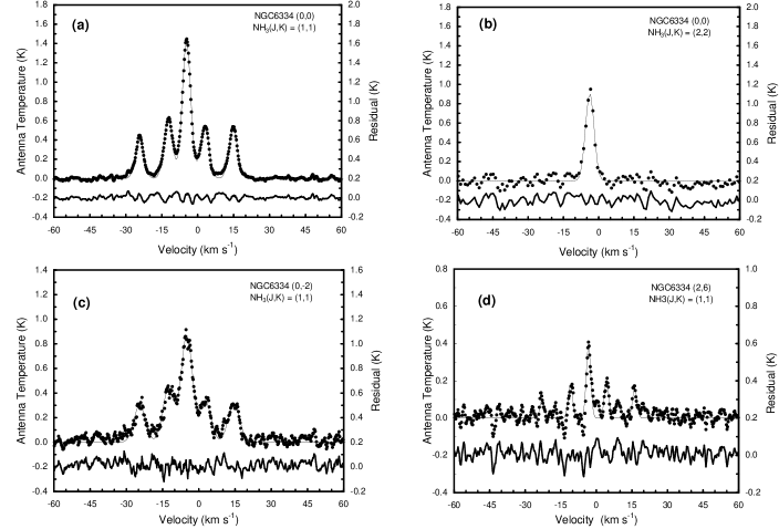
Figure 1: Spectra from the central ($\Delta\alpha,\Delta\delta$) = (0′,0′) position for the transitions (a) NH₃(J,K) = (1,1) and (b) (2,2). The NH₃(J,K) = (1,1) spectrum from the (c) (0′,-2′) and (d) (2′,6′) positions are also shown. The thin lines represent the Gaussian fittings, while the lines, below the observed spectra, are the residuals.

The NH₃(J,K) = (1,1) spectra in all the observed positions exhibit systematic differences between the line intensities in each pair of hyperfine transitions (F=1$\rightarrow$0, F=0$\rightarrow$1) and (F=1$\rightarrow$2, F=2$\rightarrow$1), which are, at least in the strongest points, much larger than the rms measured at the baseline. These intensity differences can be interpreted as the signature of non-LTE conditions. However, we should point out that this conclusion cannot be obtained by looking only at the residuals of the line fittings, which present larger rms than the baseline, both under LTE and non-LTE assumption. This is expected an expected result, since the superposition of sources and the existence of velocity gradients can make the line shapes differ from Gaussian functions.

The antenna temperature distribution and gradients of velocity and line-width are presented in Figure 2. They agree with the results of Forster et al. (for87 (1987)) and Kuiper et al. (kui95 (1995)), who mapped with high spatial resolution a small region (about 100″ in diameter) around the central position in our map in the NH₃(J,K) = (3,3) transition. However, the distribution of velocities differs from that found by Schwartz et al. (sch78 (1978)), since their map do not show an increase in the velocity’s modulus towards negative declinations, possibly due to the low signal-to-noise ratio in their spectra.

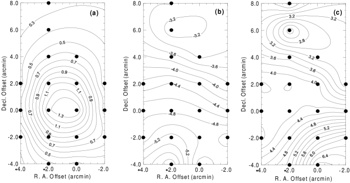
Figure 2: Maps of (a) antenna temperature (in units of K), (b) velocity (in units of km s^-1) and (c) line-width (in units of km s^-1) for the NGC 6334 region. The (0′,0′) position has coordinates $\alpha(1950)=17^{h}17^{m}32^{s}$ and $\delta(1950)=-35\degr 42\arcmin$. The black dots mark the observed positions.

3 Results

3.1 Identification of the sources NGC 6334 I, NGC 6334 I(N)w and NGC 6334 I(N)e

Although the map in Figure 2 seems to be consistent with the presence of a single source centered in NGC 6334 I(N), high resolution observations (JHH88; Kraemer & Jackson krja99 (1999)) showed the existence of at least two ammonia features, with angular sizes of the order and smaller than 1′, centered at the positions of the continuum sources NGC 6334 I(N) and NGC 6334 I respectively. Taking into account the half-power beam width of the Itapetinga radio telescope, we find that the expected contribution of these two sources at the position ($\Delta\alpha,\Delta\delta$) = (2′,6′) [hereafter, just (2′,6′)] should fall below the detection limit given by the rms of the observations. Since this is not the case, as can be seen in Figure 1(d), we conclude that another source is present in the region. We will describe, in the following paragraphs, the procedure used to separate the contribution of each component.

NGC 6334 I, when observed with high resolution (JHH88), exihibts two main structures, with velocities centered in -6.6 and -9.4 km s^-1 and widths of 2.0 and 3.5 km s^-1 respectively. The maximum flux densities of these structures are 0.42 and 0.48 Jy beam^-1 respectively which, once diluted into the 4.2′ Itapetinga radio telescope beam, correspond to antenna temperatures of 0.20 and 0.23 K respectively. We calculated the contribution of this source to the NH₃(J,K) = (1,1) spectra in our map as the convolution of the antenna beam and two point sources, with the characteristics mentioned above. The intensity of the hyperfine satellite lines was calculated assuming LTE in an optically thin source. Although the antenna temperature of NGC 6334 I is small compared to the intensity of NGC 6334 I(N), its effect on the line-width is significant, and its subtraction decreased the observed gradient along the map.

Since the high resolution observations of Kraemer & Jackson (krja99 (1999)) have revealed NGC 6334 I(N) as an extended source, although smaller than the Itapetinga radio telescope beam, it was difficult to subtract its contribution to expose the third and much weaker source. For this reason we used the spectrum at position (2′,6′), where we did not expect any contribution from the strongest source, as representative of the spectrum of the weakest. We labeled these sources as NGC 6334 I(N)w and NGC 6334 I(N)e [hereafter, I(N)w and I(N)e] respectively. We assumed no velocity gradients and subtracted a fraction of the (2′,6′) spectrum from all the others. This fraction was chosen in such a way that the resultanting spectra had the same departure from LTE as found at position (0′,0′). Moreover, since there is a velocity gradient along the region, the subtracted fraction was also limited in order to avoid fake absorptions in the resulting spectra.

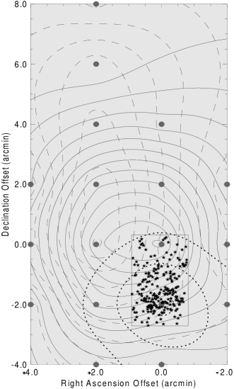
Figure 3: The superposition of the contribution of the three sources: NGC 6334 I (dotted lines), I(N)w (solid lines) and I(N)e (dashed lines). The contours are given in antenna temperature, starting at 0.1 and ending at 1.3 K (with spacing of 0.1 K). The gray points mark the observed positions. The rectangle shows the area that was observed by Tapia et al. tap96 (1996) in the JHK bands. The black stars are the sources which are detected by these authors.

In Figure 3, we show the superimposed antenna temperature maps of the three regions, NGC 6334 I, I(N)w and I(N)e. We can see that I(N)w is aproximately 2.5 and 6.5 times brighter than I(N)e and NGC 6334 I, respectively. The source I(N)w turned out to be smaller than the beam size, as expected from the observations of Kraemer & Jackson (krja99 (1999)). On the other hand, the I(N)e region looks more elongated in declination.

The subtraction procedures affected the magnitude of the gradients of velocity and line-width, but not their directions. In fact, the gradients became softer than before, showing that the other sources were responsible in some amount for the variations of these properties along the region I(N)w. As it can be seen in Figure 4, the velocity gradient is aproximately perpendicular to the Galactic plane. According to the model adopted here, the gradient in line-width is related to gradient in turbulence, which turned out to be larger in the direction of the more evolved sources.

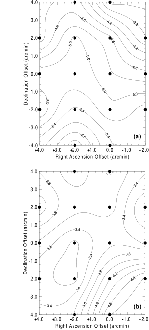
Figure 4: The gradients of (a) velocity and (b) line-width for region I(N)w. The black points mark the observed positions. The countour values are given in units of km s^-1.

3.2 The physical parameters of I(N)w and I(N)e regions in non-LTE conditions

We used the antenna temperature of the hyperfine satellites relative to the main line in the NH₃(J,K) = (1,1) spectrum and the ratio between the antenna temperatures of the main lines of NH₃(J,K) = (2,2) and (1,1), shown in Table 2, to calculate the relevant physical parameters for the I(N)w and I(N)e regions. We applied the model of SW85 to obtain the NH₃ column density ($N_{\mathrm{NH_{3}}}$), the kinetic temperature ($T_{\mathrm{K}}$) and the H₂ density ($n_{\mathrm{H_{2}}}$) of the clumps in the two regions. In region I(N)w we used the spectrum from the (0′,0′) position, which corresponds to the highest intensity, and in I(N)e we used the (2′,6′) position, where we believe there is not important contribution from I(N)w.

To determine the physical parameters of the clumps we looked into the ($N_{\mathrm{NH_{3}}}$, $n_{\mathrm{H_{2}}}$, $T_{\mathrm{K}}$) space for the point at which, according to the model of SW85, the curves representing the observed line intensity ratios intercept themselves. We had to extrapolate these curves up to H₂ densities of 10⁸ cm^-3 to obtain a good crossing point, which occured at $n_{\mathrm{H_{2}}}\sim 10^{7.5}$ cm^-3.

In Figure 5, we show the curves of constant ratio between the hyperfine satellites and the main line in the NH₃(J,K) = (1,1) spectrum, as well as the ratio between the main line intensities of the NH₃(J,K) = (2,2) and (1,1) transitions for a kinetic temperature of 24 K, which corresponds to the best fit in both regions. In Table 3, we present the values of the physical parameters extracted from this figure: the brightness temperature for the NH₃(J,K) = (1,1) and (2,2) transitions [$T_{\mathrm{B}}(1,1)$ and $T_{\mathrm{B}}(2,2)$, respectively], the kinetic temperature, the NH₃ column density and the H₂ density. We can see that the physical conditions of the clumps in both regions are pratically the same. It is important to stress that the values listed in Table 3 would not change substantially if we use the original spectra, including the contribution of the three sources, since I(N)w is much brighter than the others. On the other hand, the dispersion of the contours around the intersection point in Figure 5(a) decreased appreciably after the separation of the three components, resulting in a better accuracy in the determination of the physical parameters of the region.

Table 2: Ratio between the observed antenna temperatures of each hyperfine satellite in relation to the (1,1) main line [$T_{\mathrm{A}}^{m}$], besides the ratio between the antenna temperature of the (2,2) and (1,1) main lines.

	NGC 6334 I(N)w	NGC 6334 I(N)e
$T_{\mathrm{A}}$(F=1$\rightarrow$0) / $T_{\mathrm{A}}^{m}$	0.295 $\pm$ 0.008	0.34 $\pm$ 0.09
$T_{\mathrm{A}}$(F=1$\rightarrow$2) / $T_{\mathrm{A}}^{m}$	0.409 $\pm$ 0.008	0.47 $\pm$ 0.09
$T_{\mathrm{A}}$(F=2$\rightarrow$1) / $T_{\mathrm{A}}^{m}$	0.371 $\pm$ 0.008	0.50 $\pm$ 0.09
$T_{\mathrm{A}}$(F=0$\rightarrow$1) / $T_{\mathrm{A}}^{m}$	0.364 $\pm$ 0.008	0.42 $\pm$ 0.09
$T_{\mathrm{A}}$(2,2) / $T_{\mathrm{A}}^{m}$	0.67 $\pm$ 0.04	-

3.3 Physical parameters of the individual clumps

As it was previously mentioned, to explain the hyperfine structure intensity anomalies in the NH₃(J,K) = (1,1) transition by the superposition of individual clump spectra, their dispersion velocities must be small, implying that they should be gravitationally stable. Therefore, their individual masses ($M_{\mathrm{cl}}$) cannot be larger than the Jeans mass ($M_{\mathrm{J}}$) and their diameters ($L_{\mathrm{cl}}$) must be smaller or equal than the Jeans length ($L_{\mathrm{J}}$). Arguments in favor of these hypotheses have been presented by Curry & McKee (cumc00 (2000)) based on numerical simulations. Assuming spherical clumps with a ratio of helium to molecular hydrogen of 0.25, we calculated their diameter and mass, using the following expressions:

$$L_{\mathrm{cl}}=L_{\mathrm{J}}=\sqrt{\frac{\pi\,k\,T_{\mathrm{K}}}{7.2\,G\,m_{\mathrm{H}}^{2}\,n_{\mathrm{H_{2}}}}}\$$ (1)

$$M_{\mathrm{cl}}=M_{\mathrm{J}}=\frac{\pi}{2}m_{\mathrm{H}}\,n_{\mathrm{H_{2}}}\,L_{\mathrm{cl}}^{3}\$$ (2)

where $k$ is the Boltzmann’s constant, $m_{\mathrm{H}}$ the mass of hydrogen atom and $G$ the gravitational constant.

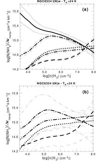
Figure 5: Ratio between the intensity of the satellites and the main line of the NH₃(J,K) = (1,1) spectrum, represented by: dashed, dashed dotted, dashed dotted dotted and dotted lines (corresponding to F=1$\rightarrow$0, F=1$\rightarrow$2, F=2$\rightarrow$1 and F=0$\rightarrow$1 transitions, respectively) for a kinetic temperature of 24 K. The upper and lower plots [(a) and (b) respectively] are associated to the I(N)w and I(N)e in this order. Ratio between the main lines intensity of the NH₃(J,K) = (2,2) and (1,1) transitions is shown by the solid lines. The weaker lines are the uncertainties associated to the fitting. The locus where these curves intersect each other represents the physical parameters of the region.

The beam filling factor ($f_{\mathrm{JK}}$) can be calculated from the brightness temperature, $T_{\mathrm{B}}(J,K)$, derived from the model and $T_{\mathrm{B}}^{obs}(J,K)$, obtained from the observations, which is proportional to the antenna temperature:

$$f_{\mathrm{JK}}=\frac{T_{\mathrm{B}}^{obs}(J,K)}{T_{\mathrm{B}}(J,K)}=\frac{2\,c^{2}}{\pi\,k\,\nu^{2}}\frac{A}{\theta_{\mathrm{B}}^{2}}\frac{T_{\mathrm{A}}(J,K)}{T_{\mathrm{B}}(J,K)}\$$ (3)

where $\theta_{\mathrm{B}}$ is the half-power beam width of the telescope and $A$ is the ratio between flux density and antenna temperature of a continuum point source. In this work, we used the radio galaxy Virgo A as the calibrating source.

Using the definition of beam filling factor, we can determine the number $K_{\mathrm{cl}}$ of clumps inside the beam’s solid angle:

$$K_{\mathrm{cl}}=f_{\mathrm{JK}}\left(\frac{D\,\theta_{\mathrm{B}}}{L_{\mathrm{cl}}}\right)^{2}\$$ (4)

where $D$ is the distance from the cloud.

To obtain the density of clumps ($\zeta_{\mathrm{cl}}$), we can consider two different situations. The first one corresponds to the clumps spread over a solid angle larger than the beam. In this case, the density of clumps is given by:

$$\zeta_{\mathrm{cl}}=\frac{4}{\pi}\frac{K_{\mathrm{cl}}}{D^{3}\,\theta_{\mathrm{B}}^{2}\sqrt{\theta_{\mathrm{\alpha}}\,\theta_{\mathrm{\beta}}}}\$$ (5)

where $\theta_{\mathrm{\alpha}}$ and $\theta_{\mathrm{\beta}}$ are, respectively, the extension of the region in right ascension and declination. In the second one, if the source is smaller than the antenna beam, we can only estimate either an upper limit, considering that the clumps are grouped side by side and without superposition, or a lower limit, supposing they are spread over the whole beam:

$$\frac{6}{\pi}\frac{K_{\mathrm{cl}}}{\left(D\,\theta_{\mathrm{B}}\right)^{3}}\leq\zeta_{\mathrm{cl}}\leq\frac{6}{\pi}\frac{K_{\mathrm{cl}}}{\left(D\,\theta_{\mathrm{B}}\,\sqrt{f_{\mathrm{JK}}}\right)^{3}}\$$ (6)

Table 3: The physical parameters determined from the Figure 5 for I(N)w and I(N)e regions.

	NGC 6334 I(N)w	NGC 6334 I(N)e
$T_{\mathrm{B}}$(1,1) (K)	12.6 $\pm$ 0.4	15.5 $\pm$ 1.0
$T_{\mathrm{B}}$(2,2) (K)	8.4 $\pm$ 0.6	11.6 $\pm$ 1.1
$T_{\mathrm{K}}$ (K)a	24.0 $\pm$ 0.8	24.0 $\pm$ 1.0
$N_{\mathrm{NH_{3}}}$ (1015 cm-2)	2.3 $\pm$ 0.8	2.4 $\pm$ 0.8
$n_{\mathrm{H_{2}}}$ (107 cm-3)a,b	1.8 $\pm$ 0.4	1.4 $\pm$ 0.7

• For each clump.

• According to SW85, the H₂ density derived from their model must be divided by 1.75 in order to obtain the true value for this parameter, shown in this table. The reason for this procedure is that only NH₃ - He collisions were considered in the numerical model of SW85 as excitational mechanism of the ammonia molecule.

Once the density of clumps and their diameters are known, we can calculate their collision time ($t_{\mathrm{coll}}$):

$$t_{\mathrm{coll}}=\frac{8\,\sqrt{ln2}}{\pi\,L_{\mathrm{cl}}^{2}\,\zeta_{\mathrm{cl}}\,\Delta v_{\mathrm{FWHM}}^{JK}}$$ (7)

We can also calculate the mean H₂ density ($\bar{n}_{\mathrm{H_{2}}}$), which is the density of an homogeneous cloud with mass equal to the total mass of the clumps filling the telescope beam:

$$\bar{n}_{\mathrm{H_{2}}}=\frac{M_{\mathrm{cl}}}{3\,m_{\mathrm{H}}}\zeta_{\mathrm{cl}}$$ (8)

The ammonia abundance is calculated from the following expression:

$$X_{\mathrm{NH_{3}}}=\frac{N_{\mathrm{NH_{3}}}}{L_{\mathrm{cl}}\,n_{\mathrm{H_{2}}}}$$ (9)

where it was assumed that there is not superposition between the clumps, so that the line of sight extension is equal to the diameter of each clump (SW85).

The physical parameters of the clumps in regions I(N)w and I(N)e and their respective uncertainties are listed in Table 4. The quoted errors for the mass and diameter of the clumps represent the uncertainties in the kinetic temperature and H₂ density.

The clumps in both regions have similar diameters (0.007 pc), masses (0.2 M_☉) and ammonia abundances (7$\times$10^-9). They also seem to be gravitationally bounded, since the total virial mass is about a factor of ten lower than the total mass of the clumps which are contained in the beam’s solid angle [7600 and 2100 M_☉ for I(N)w and I(N)e respectively]. The 36000 clumps of I(N)w are spread in such a way that their density is between 6000 and 33000 clumps per pc^-3, much larger than the 720 clumps per pc^-3 in the I(N)e region.

The beam filling factor for the I(N)w region is larger than expected from the NH₃(J,K) = (3,3) data presented in Kraemer & Jackson (krja99 (1999)) (around 0.10 for a beam size of 4′). The reason is that we had assumed no superposition between the clumps along the line of sight. The physical superposition required by the smaller filling factor is small enough to guarantee very little velocity superposition, in which case the spectra of the superposed clumps can be simply added.

Table 4: The physical parameters for I(N)w and I(N)e regions calculated in non-LTE conditions. The uncertainties are given in parenthesis.

	NGC 6334 I(N)w	NGC 6334 I(N)e
$L_{\mathrm{cl}}$ ($10^{-3}$ pc)	6.7(0.8)	7.5(1.7)
$M_{\mathrm{cl}}$ ($M_{\sun}$)	0.21(0.03)	0.24(0.06)
$f_{\mathrm{JK}}$	0.33(0.03)	0.10(0.01)
$K_{\mathrm{cl}}$ ($10^{3}$)	36(10)	9(4)
$\zeta_{\mathrm{cl}}$ (103 pc-3)	6(2) $\leq\zeta_{\mathrm{cl}}\leq$ 33(11)	0.72(0.36)
$t_{\mathrm{coll}}$ (105 years)	4(2) $\leq t_{\mathrm{coll}}\leq$ 22(9)	230(155)
$\bar{n}_{\mathrm{H_{2}}}$ (104 cm-3)	1.7(0.6) $\leq\bar{n}_{\mathrm{H_{2}}}\leq$ 9.5(3.4)	0.23(0.13)
$X_{\mathrm{NH_{3}}}$ (10-9)	6.2(2.3)	7.2(3.0)
$M_{\mathrm{tot}}(10^{3}M_{\sun})^{\mathrm{a}}$	7.6(2.3)	2.1(1.2)
$M_{\mathrm{vir}}(10^{3}M_{\sun})^{\mathrm{b}}$	0.67(0.06)	0.15(0.02)

• Total mass of whole clumps which are contained in the telescope beam.

• Mass obtained from the Virial Theorem.

4 Discussion

4.1 Ammonia abundance for the regions I(N)w and I(N)e

The study of ammonia abundance is important because it provides observational constrains for the chemical models that try to explain how this molecule is formed in the interstellar medium, and it may be used as an age indicator of the molecular cloud (e.g., Suzuki et al. suz92 (1992)). Although the chemical models calculate the evolution of the ammonia abundance as a function of time with a limited confidence, due mainly to the uncertainties concerning the formation of this molecule in the interstellar medium, they agree that the time necessary to reach the equilibrium abundance is approximately 10⁶ years. If depletion effects are not consider in the model, the equilibrium abundance for the ammonia molecule is 10^-7. If there is depletion, this value might be 10^-8 (Bergin et al. ber95 (1995)) or 10^-9 (Hasegawa & Herbst hahe93 (1993)), even though in this last case the abundance reaches equilibrium after 10⁸ years.

Comparing the ammonia abundances listed in Table 4 with the equilibrium abundance, we conclude that either the regions I(N)w and I(N)e have an age lower than 10⁶ years, or that ammonia depletion is important in both sources. This result was also obtained by Kuiper et al. (kui95 (1995)), assuming LTE conditions. Another relevant aspect that must be taken into account is the dependence of the equilibrium abundance on the nitrogen abundance in the interstellar medium, and therefore the gradient of nitrogen with galactocentric distance must be also considered (Vilas-Boas & Abraham viab00 (2000)).

4.2 Comparison with LTE models

In this sub-section, we will derive, under assumptions of LTE, the physical parameters of the source I(N)w and compare them with the parameters derived in section 3 under non-LTE conditions. We calculate these parameters at the (0′,0′) position because it is the only point in which the NH₃(J,K) = (2,2) transition was observed. In the LTE calculation we considered a three-level system, in order to obtain the rotational and kinetic temperatures ($T_{\mathrm{R}}$ and $T_{\mathrm{K}}$ respectively) through the equations (Ho & Townes hoto83 (1983); Walmsley & Ungerechts waun83 (1983)):

$$T_{\mathrm{R}}=-41.5\times\left[\ln\left(\frac{9}{20}\frac{\tau_{22}}{\tau_{11}}\frac{\Delta v_{\mathrm{FWHM}}^{22}}{\Delta v_{\mathrm{FWHM}}^{11}}\right)\right]^{-1}$$ (10)

$$T_{\mathrm{K}}=\frac{T_{\mathrm{K}}}{1+\left(T_{\mathrm{K}}/41.7\leavevmode\nobreak\ K\right)\ln\left[1+\frac{C\left(22\rightarrow 21\right)}{C\left(22\rightarrow 11\right)}\right]}$$ (11)

where $\tau_{11}$ and $\tau_{22}$ are respectively the optical depths in the transitions NH₃(J,K) = (1,1) and (2,2), C(22 $\rightarrow$ 21) and C(22 $\rightarrow$ 11) are the collision rate coefficients given by Danby et al. (dan88 (1988)).

To determine the optical depth, we assumed that the cloud has a spherical shape, that the excitation temperature ($T_{\mathrm{ex}}$) is the same in all hyperfine lines of the NH₃(J,K) = (1,1) spectrum (Ho & Townes hoto83 (1983)). Thus, using the ratio between the (1,1) main line and its inner hyperfine satellites, $\tau_{11}$ can be calculated from:

$$\frac{T_{\mathrm{A}}^{\mathrm{m}}(1,1)}{T_{\mathrm{A}}^{\mathrm{s}}(1,1)}=\frac{1-e\left(\tau_{11}^{\mathrm{m}}\right)}{1-e\left(\tau_{11}^{\mathrm{s}}\right)}$$ (12)

where $\tau_{11}^{\mathrm{m}}$ and $\tau_{11}^{\mathrm{s}}$ are, respectively, the optical depth for the main line and the inner satellites, with $\tau_{11}^{\mathrm{s}}$ = 0.28 $\tau_{11}^{\mathrm{m}}$ (Ho & Townes hoto83 (1983)) and $e(\tau)=2\,\tau^{-2}[1-e^{-\tau}(1+\tau)]$ (SW85). To obtain the optical depth for the NH₃(J,K) = (2,2) transition, it is necessary to substitute in (12) $T_{\mathrm{A}}^{\mathrm{s}}(1,1)$ by $T_{\mathrm{A}}(2,2)$, the antenna temperature of the (2,2) main line.

As we have less equations than unknown parameters, it is necessary to make some assumptions to solve the system. There are at least two clear alternatives: we may assume that either the excitation and rotational temperatures have the same value, or that the source fills completely the antenna beam. Here, we adopted the first alternative since high resolution observations indicate filling factors smaller than one for these sources (Kuiper et al. kui95 (1995); Kraemer & Jackson krja99 (1999); Megeath & Tieftrunk meti99 (1999)).

We present in Table 5 the physical parameters obtained under LTE and non-LTE conditions. The NH₃ column density and the ammonia abundance are not sensitive to LTE departures. The largest discrepancies are found in the kinetic and rotational temperatures. In fact, the kinetic temperature estimated under LTE conditions is about twice the value obtained in non-LTE. The optical depth of I(N)w, in both transitions, is slightly smaller than what it was found in previous studies (e.g., Forster et al. for87 (1987); Vilas-Boas et al. vil88 (1988); Kuiper et al. kui95 (1995)). We believe that the differences can be attributed to the lower signal-to-noise ratio in previous observations. The beam filling factor is larger under LTE conditions. This was already expected because under non-LTE conditions the gas is confined in clumps and not spread in a homogeneous cloud.

4.3 Evolutionary state of the regions

We will try to determine now the evolutionary state of the three regions identified in our ammonia observations. A possible way to explore this question is comparing the distribution of indicators of early stages of star formation. In Figure 3, we show the distribution of infrared sources, detected in the JHK bands by Tapia et al. (tap96 (1996)) in a small region of the mapped area. We can see a decrease in the number of infrared sources towards the region I(N)w and also the existence of a cluster of sources around NGC 6334 I, indicating that it is more evolved than I(N)w. Other observational results favorable to this scenario are the detection of an UCH ii region and the identification of a molecular bipolar outflow associated to this source (Rodríguez et al. rod82 (1982); Bachiller & Cernicharo bace90 (1990)). There are no infrared observations towards I(N)e, to indicate its evolutionary stage.

Our observations, together with the non-LTE model (SW85), show that the physical properties of the clumps in I(N)w and I(N)e are similar. However, the volume density of clumps in I(N)w ($\geq$ 6000 pc^-3) is at least a hundred times higher than in I(N)e, resulting in a collision rate which is hundred times higher in I(N)w than I(N)e. Thus, assuming that collisions result in coagulation of the fragments, which finally collapse to form stars after several collision times (SW85; Scalo & Pumphrey scpu82 (1982)), we expect that I(N)e is in a earlier star formation stage than I(N)w.

The evolution scenario proposed by SW85 and the results presented in this work indicate that the regions I(N)w and I(N)e could form in the future star clusters, similar to those detected in NGC 6334 I.

Table 5: Comparison between the physical parameters for I(N)w, calculated in LTE and non-LTE conditions.

	LTE	non-LTE
$T_{\mathrm{K}}$ (K)	44 $\pm$ 8	24.0 $\pm$ 0.8
$T_{\mathrm{R}}$ (K)	28 $\pm$ 3	18.7 $\pm$ 0.3
$\tau_{\mathrm{11}}$	1.42 $\pm$ 0.01	-
$\tau_{\mathrm{22}}$	0.71 $\pm$ 0.08	-
$f_{\mathrm{11}}$	0.88 $\pm$ 0.10	0.33 $\pm$ 0.03
$f_{\mathrm{22}}$	0.88 $\pm$ 0.10	0.33 $\pm$ 0.04
$\bar{n}_{\mathrm{H_{2}}}$ (104 cm-3)	12 $\pm$ 5	1.7 $\pm$ 0.6 $\leq\bar{n}_{\mathrm{H_{2}}}\leq$ 9.5 $\pm$ 3.4
$N_{\mathrm{NH_{3}}}$ (1015 cm-2)	2.5 $\pm$ 0.1	2.3 $\pm$ 0.8
$X_{\mathrm{NH_{3}}}$ (10-9)	3.3 $\pm$ 1.7	6.2 $\pm$ 2.3

5 Conclusions

The NH₃(J,K) = (1,1) spectra from the NGC 6334 region exhibit hyperfine structure intensity anomalies, suggesting departures from LTE conditions. We have used the numerical model of SW85, based on the qualitative model of Matsakis et al. (mat77 (1977)) to calculate the physical parameters of the ammonia clouds. This model takes into account the non-LTE effects through selective trapping in the far IR transition NH₃(J,K) = (2,1) $\rightarrow$ (1,1) and hyperfine selective collisional excitation. Its main limitation is that it does not include the effects of an IR continuum at the NH₃(J,K) = (2,1) $\rightarrow$ (1,1) transition frequency. As it was stressed by SW85, its influence on the anomalies is difficult to predict, but they argued that if the IR radiation field had significant influence, variations in their strength with the distance from the exciting source would be seen, which is not supported by observations, at least in the regions S106 and W48.

The existence of clumps with very small dispersion velocity was questioned by Gaume et al. (gau96 (1996)), based on the NH₃ absorption spectra in the direction of the continuum source DR21. They proposed, instead, inflows and outflows of matter in different regions of the cloud. However, the mechanism producing the non-LTE level population is the same as in Matsakis et al. (mat77 (1977)), that is, the selective trapping of photons in the NH₃(J,K) = (2,1) $\rightarrow$ (1,1) transition. Since this model was not developed quantitatively, it is not clear if it will work to explain the observed anomalies.

Although our observations do not have high angular resolution, our high quality spectra allow the identification of three distinct sources. The first one is NGC 6334 I, a compact source mapped in NH₃(J,K) = (1,1) transition by JHH88, reveling the presence of a possible bipolar molecular outflow in NH₃ and CO (Bachiller & Cernicharo bace90 (1990)), having also a cluster of IR sources (Tapia et al. tap96 (1996)). The second region is NGC 6334 I(N)w, which also presents a bipolar molecular outflow in SiO (Megeath & Tieftrunk meti99 (1999)), is the most intense ammonia source in the sky, but is not spatially resolved in our observations. It is formed by clumps with diameters of 0.007 pc, masses of 0.2 M_☉, kinetic temperatures of 24 K and with a total mass of about 7600 M_☉. This result suggests larger masses for this region than estimated by Kuiper et al. (kui95 (1995)), assuming LTE conditions. It also exihibits velocity gradients almost perpendicular to the Galactic plane, and line-width gradients parallel to the Galactic plane, showing larger line-widths towards the more evolved sources. Finally, the region NGC 6334 I(N)e is formed by clumps with physical conditions similar to those observed in I(N)w, and spread through an area larger than the telescope beam.

The ammonia abundances in both regions are similar. Their values indicate that the regions have either ages smaller than 10⁶ years or that depletion effects are important.

Among the three regions identified, NGC 6334 I is the most evolved while NGC 6334 I(N)e is in a very early star formation stage.

Comparison between physical parameters determined under LTE and non-LTE conditions showed that the NH₃ column density and ammonia abundance are the only quantities which are similar between them. Other parameters, as rotational and kinetic temperatures, exhibit differences that can reach a factor of three.

- (1) Abraham, Z., Kokubun, F., 1992, A&A, 257, 831.
- (2) Bachiller, R., Cernicharo, J., 1990, A&A, 239, 276.
- (3) Batrla, W., Wilson, T. L., Bastien, P., Ruf, K., 1983, A&A, 128, 279.
- (4) Bergin, E. A., Langer, W. D., Goldsmith, P. F., 1995, ApJ, 441, 222.
- (5) Cheung, L., Frogel, J. A., Gezari, D. Y., Hauser, M. G., 1978, ApJ, 226, L149.
- (6) Curry, C. L., Christopher, F. M., 2000, ApJ, 528, 734.
- (7) Danby, G., Flower, D. R., Valiron, P., Schilke, P., Walmsley, C. M., 1988, MNRAS, 235, 229.
- (8) De Pree, C. G., Rodr guez, L. F., Dickel, H. R., Goss, W. M., 1995, ApJ, 447, 220.
- (9) Forster, J. R., Whiteoak, J. B., Gardner, F. F., 1987, Astron. Soc. Austr., 7 (2), 189.
- (10) Forster, J. R., Caswell, J. L., 1989, A&A, 213, 339.
- (11) Gaume, R. A., Mutel, R. L., 1987, ApJS, 65, 193.
- (12) Gaume, R. A., Wilson, T. L., Johnston, K. J., 1996, ApJ, 457, L47.
- (13) Gezari, D. Y., 1982, ApJ, 259, L29.
- (14) Hasegawa, T. I., Herbst, E., 1993, MNRAS, 261, 83.
- (15) Haynes, R. F., Caswell, J. L., Simons, L. W. J., 1978, Aust. J. Phys. Astrophys. Suppl., 45, 1.
- (16) Ho, P. T. P., Townes, C. H., 1983, ARA&A, 21, 239.
- (17) Jackson, J.M., Ho, P. T. P., Haschick, A.D., 1988, ApJ, 333, L73. (JHH88)
- (18) Kogan, L., Slysh, V., 1998, ApJ, 497, 800.
- (19) Kraemer, E. K., Jackson, J. M., 1995, ApJ, 439, L9.
- (20) Kraemer, K. E., Jackson, J. M., 1999, ApJS, 124, 439.
- (21) Kuiper, T. B. H., Peters, W. L. III, Foster, J. R., Gardner, F. F., Whiteoak, J. B., 1995, ApJ, 446, 692.
- (22) Loughran, L., McBreen, B., Fazio, G. G., Rengarajan, T. N., Maxson, G. H., Serio, S., Sciortino, S., Ray, T. P., 1986, ApJ, 303, 629.
- (23) Matsakis, D. N., Brandshaft, D., Chui, M. F., Cheung, A. C., Yngvesson, K. S., Cardiasmenos, A. G., Shanley, J. F., Ho, P. T. P., 1977, ApJ, 214, L67.
- (24) McBreen, B., Fazio, G. G., Stier, M., 1979, ApJ, 232, L183.
- (25) Megeath, S. T., Tieftrunk, A. R., 1999, ApJ, 526, L113.
- (26) Menten, K. M., Batrla, W., 1989, ApJ, 341, 839.
- (27) Moran, J. M., Rodríguez, L. F., 1980, ApJ, 236, L159.
- (28) Neckel, T., 1978, A&A 69, 51
- (29) Persi, P., Roth, M., Tapia, M., Marenzi, A. R., Felli, M., Testi, L., Ferrari-Toniolo, M., 1996, A&A, 307, 591.
- (30) Rodríguez, L. F., Cantó , J., Moran, J. M., 1982, ApJ, 255, 103.
- (31) Scalo, J. M., Pumphrey, W. A., 1982, ApJ, 258, L29.
- (32) Schwartz, P. R., Bologna, J. M., Waak, J. A., 1978, ApJ, 226, 469.
- (33) Shaver, P. A., Goss, W. M., 1970, Aust. J. Phys. Astron. Suppl. Ser., 14, 133.
- (34) Stutzki, J., Ungerechts, H.,Winnewisser, G., 1982, A&A, 111, 201.
- (35) Stutzki, J., Jackson, J. M., Olberg, M., Barrett, A. H., Winnewisser, G., 1984, A&A, 139, 258.
- (36) Stutzki, J., Winnewisser, G., 1985, A&A, 144, 13. (SW85)
- (37) Suzuki, H., Yamamoto, S., Ohishi, M., Kaifu, M., Ishikawa, S., Hirhara, Y., Takano, S., 1992, ApJ, 392, 551.
- (38) Tapia, M., Persi, P., Roth, M., 1996, A&A, 316, 102.
- (39) Vilas-Boas, J. W. S., Abraham, Z., 2000, A&A, 355, 1115.
- (40) Vilas-Boas, J. W. S., Scalise, E.J., Monteiro do Vale, J.L., 1988, Ap&SS, 141, 339.
- (41) Walmsley, C. M. e Ungerechts, H., 1983, A&A, 122, 164.
- (42) Walsh, A. J., Burton, M. G., Hyland, A. R., Robinson, G., 1998, MNRAS, 301, 640.