STAR FORMATION HISTORY IN THE NICMOS NORTHERN HUBBLE DEEP FIELD

Abstract

We present the results of an extensive analysis of the star formation rates determined from the NICMOS deep images of the northern Hubble Deep Field. We use SED template fitting photometric techniques to determine both the redshift and the extinction for each galaxy in our field. Measurement of the individual extinctions provides a correction for star formation hidden by dust obscuration. We determine star formation rates for each galaxy based on the 1500 angstrom UV flux and add the rates in redshift bins of width 1.0 centered on integer redshift values. We find a rise in the star formation rate from a redshift of 1 to 2 then a falloff from a redshift of 2 to 3. However, within the formal limits of the error bars this could also be interpreted as a constant star formation rate from a redshift of 1 to 3. The star formation rate from a redshift of 3 to 5 is roughly constant followed by a possible drop in the rate at a redshift of 6. The measured star formation rate at a redshift of 6 is approximately equal to the present day star formation rate determined in other work. The high star formation rate measured at a redshift of 2 is due to the presence of two possible ULIRGs in the field. If real, this represents a much higher density of ULIRGS than measured locally. We also develop a new method to correct for faint galaxies or faint parts of galaxies missed by our sensitivity limit, based on the assumption that the star formation intensity distribution function is independent of redshift. We measure the 1.6 $\micron$ surface brightness due to discrete sources and predict the 850 $\micron$ brightness of all of our galaxies based on the determined extinction. We find that the far infrared fluxes predicted in this manner are consistent with the lack of detections of 850 $\micron$ sources in the deep NICMOS HDF, the measured 850 $\micron$ sky brightness due to discrete sources and the ratio of optical-UV sky brightness to far infrared sky brightness. From this we infer that we are observing a population of sources that contributes significantly to the total star formation rate and these sources are not overwhelmed by the contribution from sources such as the extremely super luminous galaxies represented by the SCUBA detections. We have estimated the errors in the star formation rate due to a variety of sources including photometric errors, the near-degeneracy between reddening and intrinsic spectral energy distribution as well as the effects of sampling errors and large scale structure. We have tried throughout to give as realistic and conservative an estimate of the errors in our analysis as possible.

1 Introduction

Determination of the history of the star formation rate per comoving volume in the Universe is the focus of a great deal of current research. Initial studies measuring the UV fluxes of galaxies indicated a peak in the star formation rate at a redshift near 1.5 (Madau et al. (1996)) whereas more recent studies favor a roughly constant star formation rate from a redshift of 1.5 back to a redshift of four (Steidel et al. (1999), Sawicky, Lin and Yee (1997), Pascarelli, Lanzetta and Fernandez-Soto (1998)). Further support for this conclusion comes from submillimeter observations of the HDF (Hughes et al. (1998)) and other regions (Smail, Iveson and Blain (1997), Barger et al. (1998), Ivison et al. (2000) and Barger, Cowie, and Richards (2000)). The submillimeter emission is a measure of the UV and optical flux absorbed by dust in the galaxies and reemitted at longer wavelengths. In fact, uncertainty in the amount of extinction of the UV light is a major limitation in the use of the 1500 angstrom flux as a measure of star formation rates in a galaxy.

More recent work by Madau, Pozzetti and Dickinson (1998) indicates that the falloff of the star formation rate is not as steep as first thought, but is still present in the range of redshifts between 2 and 4. Madau 1999, however, points out that “If stellar sources are responsible for the photoionization of the intergalactic medium at a redshift of $\approx 5$ then the rate of star formation at this epoch must be comparable to or greater than the one inferred from optical observations of galaxies at $z\approx 3$”. Galaxies with redshifts greater than 5 are indeed observed (Dey et al (1998), Weymann et al. (1998)) so that reionization due to galaxy starlight may well have occurred before that epoch. In fact, the recently discovered QSO by Stern et al. (2000) clearly indicates that reionization had already occurred to some degree at a redshift of 5.5.

A key to greater accuracy in measuring the star formation rate history is a determination of both the extinction and redshift of the galaxies used in the analysis. Madau (1999) uses a single correction for dust absorption of A${}_{1500}=1.2$ mag for all of the galaxies in his sample except for the redshift 0.75 to redshift 1.75 galaxies where the equivalent extinction at 2800 angstroms is used. Steidel et al. (1999) make corrections for dust absorption by assuming that any color deviations in their sample galaxies are solely due to dust absorption, based upon work of Meurer, Heckman, and Calzetti (1999). These authors derived an empirical relation between the slope of the observed UV spectrum and the far infrared emission to correct their star formation rates. In this paper however, we measure the extinction of each galaxy in our sample without the assumption of a uniform UV spectral energy distribution for all star-forming galaxies.

This work focuses on the portion of the northern Hubble Deep Field (HDF) covered by deep observations with the Near Infrared Camera and Multi-Object Spectrometer (Thompson et al. (1999)). These observations have the disadvantage of small areal coverage. However, this portion of the HDF has the significant advantage of deep photometric images in six wavelength bands, four from the original WFPC2 study (Williams et al. (1996)) and two from NICMOS imaging. The presence of the two infrared bands facilitates the technique of photometric redshift determination and the extension of the wavelength range to more than a factor of 5 provides the opportunity for extinction measurement.

Our analysis of the star formation rate in the deep NICMOS HDF thus consists of two parts. The first is a traditional analysis of the star formation rates via photometric redshift measurements of the galaxies by matching numerically redshifted standard spectral energy distribution templates, but without any correction for internal dust extinction. This is similar to the approach used by Fernandez-Soto, Lanzetta and Yahil (1999) and others. (A recent summary of various photometric redshift techniques may be found in Weymann et al. (1999).) The second part expands on this by including extinction as well as redshift in the templates in an attempt to reduce the uncertainty in the true UV flux of a galaxy caused by dust extinction.

The plan of the rest of the paper is as follows: In section 2 we describe the data set and its photometry. Section 3 contains the methodology we use to measure redshifts, extinction and stellar population types. Section 4 presents the results for the redshifts and extinction. In section 5 we show the resultant star formation rates measured from our template fitting. These fits are of course subject to both photometric errors and template errors. Section 6 addresses these issues, including the issue of near-degeneracy between extinction and template type. Section 7 presents particularly interesting or problematic galaxies. In addition to errors in our fits, the star formation rates at high redshifts must be corrected for incompleteness due to both star formation occurring in galaxies too faint to be detected and in portions of galaxies whose surface brightness is below our detection threshold. This is discussed in section 8 where we apply a correction both through standard luminosity function and aperture corrections, as well as by a new method using an empirical form of the “star formation rate surface density distribution function”, recently discussed by Lanzetta et al. (1999). Our final numbers for the star formation history versus redshift are presented in this section. Section 9 presents a prediction of the far infrared fluxes expected for the galaxies in our list. In section 10 we examine the errors due to large scale structure and small number statistics. We discuss in section 11 the comparison between our findings and the results from optically based studies, the possible evolution of the surface brightness of galaxies and the consistency between our results and those from submillimeter and far infrared measurements. Also we comment on the relation of our work to some recent models for star formation in the early universe. We end with a brief set of conclusions in section 12.

We adopt throughout this paper an open Friedman cosmology with $H_{o}=65$ and $\Omega_{o}=0.3$.

2 Observational Data

The data set for this work comes from the NICMOS and WFPC2 observations of the northern HDF. The NICMOS images used in this analysis are the IRAF–generated F110W and F160W images described in Thompson et al. (1999).

2.1 Object Selection and Photometry

Szalay, Connolly, and Szokoly (1999) describe a method for combining images from several wavebands which gives appropriate weights to the various images. We have followed the Szalay et al. 1999 procedure for selecting galaxies, a subset of which comprise the galaxies discussed in this paper.

The F160W and F110W images were trimmed from their original 512 x 512 $0.1\arcsec$ drizzled pixel sizes to 481 x 486, eliminating the outer regions of the frames where the dither pattern caused these regions to be much noisier than the inner regions. The four WFPC2 images were then transformed to the same pixel coordinate system as the NICMOS images by measuring a large number of compact objects and using the IRAF tasks GEOMAP and GEOTRAN. The transformation has an accuracy of about 0.02″, with the uncertainties probably dominated by intrinsic differences in the centroids for the different bandpasses. Next, we convolved the transformed WFPC2 images with a gaussian whose width was chosen such that the radial profile of the central star (WFPC 4-454, NICMOS 145.0) in the images closely matched the radial profile in the F160W image. While the agreement of these resultant radial profiles is not perfect, this procedure should be adequate for the fluxes used to carry out the template fitting described in this paper.

We next laid down a grid of points where we placed bright artificial point sources and then used the program SExtractor (Bertin and Arnouts (1996)) to determine the background and local $\sigma$ at these grid points. We then fit these grids with 2D Chebychev polynomials to define the background and $\sigma$ at every point in the 6 frames.

Each of the 6 frames is then normalized to have zero background and unit variance. This must be done locally, especially for the NICMOS frames, since the S/N varies substantially across the image and there are also small residual background variations in the reduced images described above. From these 6 frames we produced a single (weighted) $\chi^{2}$ map and selected a threshold in $\chi^{2}$ for identifying the pixels in the map that lie above that threshold. Since we are interested in extending our analysis to quite high redshifts, we gave the F300W and F450W images zero weight, since except for very blue low redshift objects these two bands contribute little to the final selection of objects and at high redshifts simply increase the noise. In fact, there is very little difference in the maps produced with weighting equally the F606W, F814W, F110W and F160W images and assigning zero weight to the F606W image. In the following we use the maps formed from just the F814W, F110W and F160W images.

We selected a threshold of the Szalay R parameter, $R=\sqrt{\chi^{2}}=2.3$, as the significance level for “real” pixels and required 3 contiguous pixels (ie for the SExtractor parameter DETECT MINAREA) for selecting a preliminary list of objects. With these parameters, SExtractor detected 365 objects.

We then measured fluxes with SExtractor in an $0.6\arcsec$ diameter aperture at the centroid found by SExtractor from the $\chi^{2}$ image. Apertures larger than this admit too much sky for the faint objects and increase the risk of contamination from nearby galaxies. For apertures much smaller than this, registration and PSF matching become concerns. The determinations of the redshift and extinction for each galaxy described in section 3 utilize these fixed aperture fluxes. However, in order to estimate the total UV flux associated with each galaxy, aperture corrections must be applied. We perform the aperture corrections in two different ways. First using the aperture correction method described in Yan et al. (1998) and second with a new method that uses the distribution function of the star formation intensity.

For our template fitting algorithm, we also require an estimate of the $\sigma$’s associated with the 0.6″  aperture fluxes. As noted, this does not scale simply with the square root of the number of pixels in the aperture. We have thus used an entirely empirical estimation by again laying down a grid (avoiding the “significant pixels”), and determining empirically the $\sigma$ found for blank sky regions by SExtractor through the 0.6″ aperture for many locations within each grid point, and again fitting this grid of $\sigma$’s with a 2D Chebychev polynomial.

Small remaining errors in the local background and/or $\sigma$, may still cause spurious objects to appear. We therefore imposed the following additional criteria to select a subset of these objects. We required that all selected galaxies have at least one band with an $0.6\arcsec$ aperture signal–to–noise value greater than or equal to 3.5. and at least two bands with signal to noise values greater than or equal to 2.5. As shown by Hogg and Turner (1998) objects noisier than this are subject to a systematic overestimate of their true flux. There will be a systematic bias in the measured flux when the number counts increase with increasing magnitude. These authors suggest that objects with signal to noise less than $\sim$4 are of little value. We have relaxed this to 3.5 since the actual slope of the $log\,N-m$ relation is somewhat shallower than the shallowest considered by these authors. In addition, SExtractor provides warning flags for objects close to the edge of the image. There were 35 such cases and after careful visual inspection we accepted 10 of these as having aperture fluxes not compromised by the proximity of the edge. We also removed the known star (NICMOS 145.0) and two faint spurious objects which were associated with the diffraction pattern from this star. These additional considerations reduced the preliminary list of 365 objects to 282 which form the basis of our analysis.

3 Methodology

The main output of our analysis is the most likely redshift, extinction and intrinsic spectral energy distribution (SED) for each of the galaxies that passed the selection criteria described in Section 2.1. We do this by taking a group of initial template SEDs and numerically altering them over a grid of redshift and extinction. We then use a minimum $\chi^{2}$ technique to compare the observed fluxes with templates to find the best match. Section 6 discusses the robustness of the technique and the probable errors associated with it.

3.1 Redshift Determination

Our first task in the analysis is finding the redshift for each galaxy. The paucity of spectroscopic redshifts in the field dictates a photometric technique for the redshift determination. We chose a template fitting method which includes interpolation between 6 discrete template spectral energy distributions.

3.1.1 Template versus Polynomial Fitting

Recently there has been relatively good success in the use of polynomial fitting to determine the photometric redshifts, e.g. Wang, Bahcall, and Turner (1998). This method fits a training set of known redshift object fluxes with a polynomial function of the color of the objects. Different polynomials are fit for different color regimes. This technique has an advantage of being independent of any set of assumptions on the actual SEDs of the objects. For the data considered here we have chosen instead a template fitting technique because the number of galaxies with spectroscopic redshifts and photometry in these 6 bandpasses is too small at the higher redshifts to be used as a training set.

3.1.2 Template Properties

We draw our templates from three sources. The first source is the four observed SEDs of Coleman, Wu, and Weedman (1980) utilized by several authors. The unreddened SED of the set of mean SEDs of Calzetti, Kinney & Storchi-Bergman (1994) provides an additional observed template of an active star-forming galaxy (Calzetti (1999)). A final and even hotter template is a 50 million year old continuous star formation SED calculated from the Bruzual and Charlot models (Bruzual and Charlot (1996)) with a Salpeter IMF and solar metallicity. This theoretical SED does not have any emission lines, so we have added emission lines from H$\alpha$, (O[III]+ H$\beta$) and O[II] by scaling up those associated with the Calzetti SED by the ratio of the UV fluxes in the Calzetti and Bruzual–Charlot SEDs. Template 6 is substantially bluer than the most recent unreddened SED for local star burst galaxies (cf Calzetti (1997)). Calzetti (1997) shows that stellar synthesis models evolving older and redder populations must be added to a very young population to reproduce the star burst SED. However, we find instances where our 50 million year old template (without any internal reddening) gives a much better fit than the Calzetti template, and for this reason we have added this last template. It could well be that at higher redshifts we are seeing galaxies that are so young that they have not had a chance to produce an older population. An excellent example of this is NICMOS 184.0, (WFPC 4-473) with a spectroscopically measured redshift of 5.60 (Weymann et al. (1998)). Template 6 with no extinction gives a good match to the observed fluxes and reproduces the blue F160W - F110W color of the object. Template 5 with no extinction provides a poor match and cannot reproduce the blue F160W - F110W color at the known redshift of the galaxy. We find many other objects for which an unreddened template 5.5 or hotter gives the best fit.

Figure 1 shows the spectral energy distributions of these six basic templates. The numbers run from the earliest (coolest) galaxy template (number 1) to the latest (hottest) template (number 6). We have assumed that no flux shortward of the Lyman limit escapes from any of the galaxies, and we have also neglected any flux in the Lyman $\alpha$ line. Trials with SEDs including Lyman $\alpha$ suggest that inclusion of Lyman $\alpha$ makes very little difference in the obtained fits. In addition to internal reddening from dust (described below) we also include the external attenuation from Lyman absorption, using the formulation of Madau et al. (1996).

Figure 1: Spectral energy distributions for the six discrete templates.

3.1.3 Template Interpolation

The observed galaxies will not be an exact fit to any one of the six templates. To mitigate this problem and to reduce the extinction error due to an effect described in Section 6.3, we interpolate between templates. The interpolation process is carried out on the total fluxes calculated for the filters. Once the filter fluxes for each filter are calculated for all templates, redshifts and extinctions, 9 intermediate fluxes are calculated between each template in a linear interpolation. This effectively increases the number of templates to 51. Since the average flux difference between adjacent templates is about a factor of 3 a linear interpolation should be adequate.

3.2 Extinction Law

All extinctions used in this work are from the formulation of Calzetti, Kinney & Storchi-Bergman (1994). Since this extinction law derives from observations of the integrated flux of external galaxies it has an advantage of reasonably representing the actual mix of scattering and absorption present in real galaxy observations, as well as the very complex geometry of the distribution of the hot stars and dust. The derivation of the “obscuration law” of Calzetti, Kinney & Storchi-Bergman (1994) for the integrated flux from galaxies (and our application of this law) assumes an exponential relation between the fraction of the flux transmitted at any wavelength and the color excess. This implies that the geometry of the star and dust distribution more closely resembles a “clumpy screen” than a geometry in which the dust and stars are mixed uniformly together. In the uniformly mixed case the relation between the column density of dust and the fraction of stellar radiation escaping takes on a very different form (cf their equation (19)). While it might seem naive to apply such a law to the integrated colors of an entire galaxy, more recent work (Calzetti et al. (1999)) using ISO photometry shows that this formulation is able to predict reasonably well the average thermal emission (hence the UV extinction) based upon the integrated UV slope. As these authors note, however, this result would not apply to objects whose geometrical distribution of dust is very different, such as very luminous, dusty, compact objects where a large percentage of the hot stars are heavily embedded in the dust. For such objects (e.g. the “LIRGS” and “ULIRGS”) application of the Calzetti formulation is likely to lead to a significant underestimate of the fraction of UV radiation absorbed and reradiated by the dust.

We use 15 different extinction values ranging from E(B-V) = 0 to 1.0. The range between 0.0 and 0.1 is sampled in 0.02 increments and the range between 0.1 and 1.0 in increments of 0.1. These extinctions are applied to each of the 51 filter fluxes of the SED templates to produce a total of 765 different effective templates at each of the 100 steps in redshift between 0 and 8. We choose to limit our redshift range to values less than or equal to 8 because at redshifts greater than this only the F160W band will have significant flux. Flux in only that band cannot discriminate between a high redshift galaxy and a galaxy with high extinction. Also our selection criteria for galaxies will exclude any galaxy with significant signal to noise in only the F160W band. This will exclude from our list any objects with redshifts significantly greater than 8 and very high redshift extremely reddened objects.

3.3 Modified $\chi^{2}$ Analysis

The basic technique minimizes the $\chi^{2}$ residuals between the observed fluxes and those predicted by the various templates which are numerically shifted over a grid of redshifts and subjected to internal extinction, measured by E(B-V), and the intervening Lyman attenuation. Our technique varies from that of previous workers, (e.g. Fernandez-Soto, Lanzetta and Yahil (1999)) by altering the error term in the denominator to include a term proportional to the measured flux as well as the estimated error in the measurement of the flux. Our $\chi^{2}$ residual is then given by

$$\chi(z,E)^{2}=\sum_{i=1}^{6}\left(\frac{(f_{i}-A\cdot fmod(z,E)_{i})}{\sqrt{\sigma_{i}^{2}+(0.1f_{i})^{2}}}\right)^{2}$$ (1)

In equation 1 the index i refers to the six fluxes used in this work, $f_{i}$ is the measured flux and $fmod(z,E)$ is the flux predicted by a template at a redshift of z and with an extinction value, E(B-V), equal to E. Note that this is not a formal $\chi^{2}$ calculation so the usual quantitative probabilities associated with formal $\chi^{2}$ values are not valid. The normalization constant A, is chosen to minimize the value of $\chi(z,E)^{2}$ and is given by

$$A=\sum_{i=1}^{6}\frac{f_{i}\cdot fmod(z,E)_{i}}{\sigma_{i}^{2}+(0.1f_{i})^{2}}/\sum_{i=1}^{6}\frac{(fmod(z,E)_{i})^{2}}{\sigma_{i}^{2}+(0.1f_{i})^{2}}$$ (2)

In equations 1 and 2, when the measured fluxes were negative, they were replaced by 0.0. In this form the limit of the expression at very low flux levels is the standard form with the formal background $\sigma$ dominating the denominator and at high flux levels it is the flux difference between the observations and the model divided by 10$\%$ of the flux instead of the $\sigma$. The rationale for this formulation is that at high flux levels the errors in the fit will be proportional to flux since the error will be dominated by systematic errors in the flux.

The actual accuracy of the NICMOS flux levels is higher than this and is estimated to be on the order of 1 - 2$\%$. These higher than usual accuracies are due to the nature of the observations. The deep NICMOS HDF observations are very highly dithered and are of generally extended objects. This greatly mitigates the interpixel effects described in Lauer (1999). More generally, it is our belief that in the case of relatively bright objects, the percentage error in the flux differences should be weighted equally, since all 6 bands contain important information. In any case, our results do not appear to strongly depend on the precise coefficient of the flux in the denominator of equation 1.

3.4 Zero Extinction Redshifts

The star formation rate results for zero extinction correction plotted in figure 6 use redshifts that are calculated from a set of templates that are restricted to zero extinction. This is a suite of 51 effective templates. In some cases the redshifts can differ from those calculated with extinction for reasons presented in Section 6.3.1.

4 Results

In this section we present the results of the $\chi^{2}$ analysis for the redshift and the extinction. Table 1 contains a list of the results of our analysis on all of the objects, ordered by RA. Column 1 of the table gives the NICMOS identification numbers. Objects with ID numbers less than 1000 are objects that are identified with sources in the original KFOCAS catalog of Thompson et al. (1999) and are listed by their original catalog numbers from the extended electronic version. Objects with catalog numbers greater than or equal to 1000 are SExtractor objects that did not match in position with an original catalog entry to within $0.3\arcsec$. There are several reasons for this. One reason is different morphology in the bands used to determine the position. The original catalog took the F160W band centroid as the position of the object. The current work establishes a position using the weighted sum of the F814W, F110W and F160W bands which can shift the location of the centroid. If the positional differences are greater than $0.3\arcsec$ then it is declared a mismatch. A second reason involves the difference in the way that the two programs determine parent and daughter objects. There is generally a mismatch in these cases. Finally, our current object selection procedure differs slightly from that used in Thompson et al. (1999) so that some faint objects may appear in Thompson et al. (1999) which do not appear here and vice versa.

Column 2 gives the WFPC2 identification number of the galaxy from Williams et al. (1996). Again there must be a positional coincidence within $0.3\arcsec$ for a match to be valid. Columns 3 and 4 give the determined values for the redshift and extinction. Column 5 contains the star formation rate (SFR) in solar masses per year as determined in Section 5.

The bolometric luminosity of the galaxy is in column 6. The flux of a galaxy is obtained by integrating over the unextincted selected template scaled by the factor A from equation 2. The bolometric luminosity then follows from the redshift and our adopted cosmology. The fraction of the luminosity that is extincted and therefore goes into far infrared flux is given in column 7 followed by the calculated 850 $\micron$ flux (mJy) in column 8 (cf section 9).

Columns 9 and 10 give the template number T of the best fit, and the modified $\chi^{2}$ value of the fit from Equation 1. It should be noted that the distribution of the modified $\chi^{2}$ values will not rigorously follow a true $\chi^{2}$ distribution. The values are provided to give a qualitative indication of the relative goodness of fit for the best fit values of redshift, template type and E(B-V) from object to object.

Column 11 gives the total F160W AB magnitude (Tot. mag) derived from the aperture correction method described in Yan et al. (1998) followed by the 0.6 aperture F160W magnitude (Ap. mag) in column 12. If no F160W magnitude is listed the object had a zero or negative measured F160W flux. Columns 13 and 14 are the right ascension and declination positions of the object. The RA listing contains only seconds and the DEC listing only minutes and seconds. 12$\fh$ 36$\fm$ should be added to the RA and 62$\fdg$ to the DEC. If a source has a slightly different RA in this analysis than in the original it may not appear in the same order as in the original catalog.

4.1 Redshifts

Figure 2 shows the distribution of photometric redshifts from our analysis. A check on the accuracy of our methodology and set of templates is a comparison with the known spectroscopic redshifts in the deep NICMOS region of the Hubble Deep Field (Cohen et al. (2000)). Figure  3 shows that comparison. Although the number of objects with spectroscopic redshifts in the deep NICMOS region is small, the agreement is comparable to that typically achieved by the technique of photometric redshifts. (Weymann et al. (1999)).

Figure 2: Histogram of the number of galaxies versus photometric redshift

Figure 3: Comparison of the photometric and known spectroscopic redshifts for the deep NICMOS HDF.

Another check on the reasonableness of our redshift determinations is the magnitude–redshift plot shown in Figure  4. As expected, the brightest magnitude at any redshift dims with increasing redshift. The plot also shows the 0.6$\arcsec$ aperture magnitude tracks of both an early type (cool) and a late type (hot) template $L^{*}$ galaxy in the F160W magnitude versus redshift plane. These are templates 1 and 5 shown in Figure 1. We take the bolometric luminosity of an $L^{*}$ galaxy to be $3.4\times 10^{10}L_{\odot}$ and assume an exponential profile with a characteristic radius of 3.5 kpc. The dashed dot line in Figure  4 is for an extincted late–type (template 5) galaxy with E(B-V) equal to 0.2

Figure 4: The distribution of F160W AB 0.6$\arcsec$ diameter aperture magnitudes versus photometric redshift. The solid and dashed lines indicate the F160W aperture magnitude of an early and late-type L^∗ galaxy of fixed luminosity. The dash dot line shows the track of a late-type L^∗ galaxy with an extinction of E(B-V) equal to 0.2. The relevance of these plots is discussed further in section 8.1

4.2 Extinction

Figure 5 shows the histogram of extinctions. The extinction range is from E(B-V) = 0 to 1. The histograms show significantly more extinction for galaxies in the redshift range 0 to 2.0, than for galaxies at higher redshift values. This is not a real effect. Surface brightness dimming at the higher redshifts makes the galaxies so faint that high extinction galaxies fall below our detection limit. The existence of highly extincted galaxies at high redshift have been confirmed by SCUBA observations discussed in section 11.2.2. The distribution of extinctions in Figure 5 differs from the distributions of extinction shown in Figure 10 of Adelberger and Steidel (2000). In Adelberger and Steidel (2000) the extinction distribution is based on the value of the observed UV slope $\beta$ relative to a nominal slope. Galaxies bluer than the nominal $\beta$ are assigned negative extinction values and the distribution is roughly symmetric about 0. In our analysis we determine the best value of the intrinsic UV slope in our template choice and then only allow positive extinction values to produce the observed UV slope.

The 0.0 - 0.1 bin in Figure 5 contains the 5 E(B-V) values of 0.0, 0.02, 0.04, 0.06, and 0.08, while the 0.1 - 1.0 E(B-V) values are spaced in intervals of 0.1. There is an overdensity of objects with calculated E(B-V) values of 0.0. This may be due to galaxies which are bluer than our hottest template. Even if the galaxy does have some reddening the best template match will be our hottest template with no reddening. We have also assigned the Coleman, Wu, and Weedman (1980) galaxies zero extinction although they must suffer some extinction. Real galaxies with similar SEDs but less extinction will then also be assigned zero extinction in our procedure.

Figure 5: Histogram of the photometrically determined E(B-V) values.

5 Measured Star Formation Rate History

We determine the observed 1500 Å rest frame flux via the methods described below. This flux then determines the observed star formation rate for the galaxies in this sample. The rates so determined must be corrected for incompleteness, as described in Section  8.

5.1 Relation Between Star Formation Rates and the Ultra-Violet Flux

This work utilizes the relationship between the star formation rate and the UV flux at 1500 Å given by Madau, Pozzetti and Dickinson (1998).

$$UV_{1500}=8.0\times 10^{27}\cdot SFR(M_{\odot}/yr)\ \mathrm{ergs\ second^{-1}\ Hz^{-1}}$$ (3)

The 1500 Å UV flux is determined from the redshift, the extinction and UV flux of the best fitting template and the scale factor A determined from the measured flux of the galaxy (equation 2). The UV flux of the template is used as a measure of the UV flux of the actual galaxy. We use this flux rather than the measured flux since for low redshifts the 1500 Å flux is not directly measured and at higher redshifts the F300W and F450W fluxes often have relatively high errors. Also, since the correction for extinction is a primary goal of this work, we must use the template flux to measure the intrinsic UV flux in the absence of extinction. Finally since the Madau UV flux to star formation rate is a narrow band relation we must use the template values to relate the flux in the wide photometric band to the narrow band UV flux at 1500 angstroms.

The relationship in Equation 3 is dependent on the initial mass function (IMF) and therefore may be different at earlier times than at present. In particular the IMF may be weighted toward higher mass stars at high redshift when the metal content of the star forming material may be less. This effect would produce a higher UV flux for a given star formation rate leading to an over estimation of the rate. This would work in the opposite sense from the likely underestimate of the star formation rate for the very dusty luminous objects mentioned in Section  3.2.

Figure 6 shows the combination of all of the analyses from above. Galaxies with redshifts less than 0.5 are not included in Figure  6. Large area surveys of local galaxies are much more accurate in determining that result than the small area surveyed here. The star formation values shown in Figure 6 must still be corrected for luminosity missed due to surface brightness dimming (section 8). The error bars in figure 6 reflect only those errors caused by errors in photometry as discussed in Section  6. Other error sources are discussed in several following sections and are included in the final results shown in Figure 16.

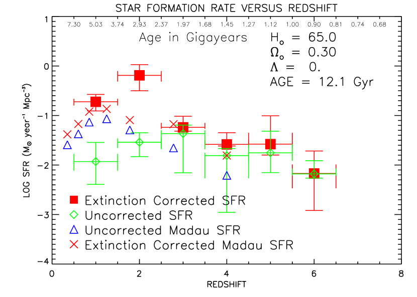
Figure 6: Star formation rate per comoving volume with and without correction for the extinction as a function of redshift. The star formation rates have not been corrected for missing luminosity and the error bars reflect only those errors caused by errors in photometry. Figure 15 shows the luminosity corrected star formation rates and full error bars.

There are several interesting features in Figure 6. It is evident that our measured star formation rate in the 0.5 to 1.5 redshift bin, without the extinction correction, is very much lower than the uncorrected rate found by Madau (1999), as shown by the triangles. This may be in part due to our selection criteria for the deep NICMOS field. In order to provide the best field for slitless grism spectroscopy we deliberately chose a field that was the least dense in large, bright and therefore relatively nearby objects. As we will discuss below most of the star formation rate is usually contributed by a relatively small number of highly luminous objects. Our field selection was biased against precisely such objects.

A second feature is the large correction for extinction present in the lowest two redshift bins. This qualitatively follows the trend seen in Figure 5 where the extinction is significantly higher for low redshift objects than higher. Note that our field selection was performed on the WFPC2 image so we are not biased against nearby faint, highly extincted but intrinsically bright galaxies. Table 2 shows the 10 highest contributors to the star formation rates in each redshift bin along with their identification numbers from Table 1. If we look at the primary contributors to the increased star formation rate in the lowest redshift bin (z = 0.5 - 1.5) we find that approximately one third of the rate is provided by one galaxy (ID = 49.0) which has an E(B-V) value of 0.5. 29 galaxies out of the 81 in the bin contribute fluxes that make up $90\%$ of the total star formation rate, however, the 3 brightest galaxies contribute more than 50$\%$ of the flux. For consistency we note that the spectroscopic redshift of galaxy 49.0 is 0.45 which would move it out of our lowest redshift bin while our photometric redshift of 0.56 moved it into the bin. We choose not to adjust by hand those objects with known redshifts.

In the second lowest redshift bin (z = 1.5 - 2.5) 5 of 52 galaxies contribute $90\%$ of the total corrected star formation rate. One galaxy (NICMOS 166.0) contributes almost half of the flux and another (NICMOS 277.211) contributes another third of the flux. NICMOS 166.0 and 277.211 have E(B-V) values of 1.0 and 0.7 respectively and it is the extinction correction applied to these two galaxies that produces the high star formation rate for this redshift bin. Inspection of the image confirms that both galaxies are extremely red with significantly higher near infrared flux than visible. Note that the equal extinction correction applied by Madau (1999) greatly underestimates the star formation rate for these galaxies. In section 9 we will find that these two galaxies may be ULIRGs. The implication of this is discussed in section 7.3.

6 Error Analysis

Errors in the photometry of the sources and errors due to the inadequacy of the standard templates to represent the true spectral energy distribution of an observed galaxy translate to errors in the values of the star formation rates in Figure 6. The first source of error is quantifiable while the second is more difficult to quantify.

6.1 Photometric Error

We test the sensitivity of the calculated redshifts and extinctions to photometric errors by running 100 test cases on each of the individual sources. A single test case consists of randomly altering the flux value in each wavelength band in a Gaussian distribution of errors of width determined by the $1\sigma$ values determined in the photometric reductions plus 1$\%$ of the observed flux. This gives 36,500 different cases. Several runs of this procedure produced results that were statistically indistinguishable from each other so we feel the procedure is robust.

Figure 7: Histogram of the photometric redshift errors produced from a random Gaussian distribution of flux errors. The bin size is 0.2 in redshift.

Figure 8: Histogram of the photometric extinction errors produced from a random Gaussian distribution of flux errors. The bin size is 0.1 in E(B-V).

Figure 9: The cumulative distribution of the fractional errors in derived UV luminosity produced from a random Gaussian distribution of flux errors in each redshift bin. The left and right vertical lines indicate the 16% and 84% confidence regions. The fractional error is defined as the measured redshift with perturbation minus the redshift with no perturbation divided by the no perturbation redshift.

Figures 7 and  8 show the results of one run of this procedure for the 36,500 different realizations. The distribution of errors in redshift and extinction are relatively symmetric about 0 but the low lying extension to larger errors is not consistent with a purely gaussian distribution. Large shifts in the redshift or extinction occasionally arise when a secondary minimum in the $\chi^{2}$ distribution for the measured fluxes becomes the primary minimum when the fluxes are perturbed.

To see how the star formation rates are affected, by the photometric errors, we compute the star formation rate in all redshift bins for each one of the 100 realizations. In Figure 9 we plot these distributions along with the 16% and 84% values (which would correspond to the $\pm 1\sigma$ limits if the distribution were gaussian, which it is not) and these values are used for the error bars plotted in Figure 6.

6.2 Redshift Errors Resulting from Inadequate Templates

The error due to improper templates is much harder to quantify than the errors due to photometry. As shown in Figure  3, there is excellent agreement for the small number of objects in our field for which spectroscopic redshifts exist. Typical errors in photometric redshifts for bright objects—bright compared to the majority of galaxies in our sample—(for which template errors rather than photometric errors probably dominate) are generally small compared to the error we have estimated in our set of redshifts due to errors in the photometry. See, for example, Benitez (1999), Brunner, Connolly, and Szalay (1999) , Budavari et al. (1999), Connolly et al. (1999), Lanzetta et al. (1999), Wang Bahcall and Turner (1999). We therefore neglect this error compared to the photometric error, though to be sure there may well be some isolated large excursions where an object at a small redshift is mistaken for an object at a large redshift or vice versa which can give rise to an error in the star formation rate for the galaxy.

6.3 Template-Extinction Error

Too widely spaced discrete templates can give rise to a bias in the determination of the extinction (Koo (1999)). Since negative extinctions are not allowed, there is a bias toward a higher calculated extinction than the actual value. An obvious example is a galaxy with no extinction that lies halfway in color between two templates. Since negative extinctions cannot be applied to the redder of these two templates, the only way to make a fit is to apply extinction to the bluer of the two templates. Within any grid of template and extinction there will be a similar bias toward higher extinction. To mitigate this effect, our program uses filter fluxes interpolated between the filter fluxes from the set of six primary templates, as described in Section  3.1.3.

6.3.1 Template Extinction Degeneracy

Since extinction and star formation history alter the colors of galaxies in ways which are by no means orthogonal (cf Kodama, Bell, and Bower (1999) and D. Thompson et al. (1999)) there can be a partial degeneracy in terms of extinction and template type, leading to a possible error in the derived star formation rate. This error can be present whether the extinction is explicitly determined or not. If the extinction is assumed to be zero, a galaxy undergoing vigorous star formation but suffering significant extinction may be falsely matched to an earlier type galaxy and the actual ultraviolet flux will be greater than the flux determined from the match. Conversely, if an extinction correction is attempted, an early type unreddened galaxy might be falsely matched with a heavily extincted late type galaxy, particularly in the presence of low signal to noise. The large wavelength coverage of our data mitigates the problem to a degree, however, this issue must be properly investigated. We investigate the issue in several ways, inspection of the $\chi^{2}$ distribution of a heavily extincted galaxy, examination of the differences between intrinsically red templates and extincted templates, inspection of the effect of photometric errors on the data discussed previously in section 6.1, and finally by performing a similar perturbation test on artificial data from our templates.

First, we chose a galaxy determined to be heavily extincted by our procedure, NICMOS 166, which is also discussed in Section 7.3. The extinction for this galaxy is E(B-V) = 1.0, the highest value in our grid of extinctions. Inspection of the images shows a galaxy that appears relatively faint at optical wavelengths but very bright at 1.1 and 1.6 microns.

Figure 10: The contour plot of $\chi^{2}$ in the template-extinction plane at the best fit redshift of NICMOS 166.0 (z = 1.60). Only the lowest contours are plotted for clarity. The tick marks point toward lower values of $\chi^{2}$.

The effect is shown in Figure  10 which displays the contour plot of the $\chi^{2}$ map for the galaxy NICMOS 166 in the template - extinction plane at the best-fit redshift of the object (z = 1.60). There is a clear valley of low $\chi^{2}$ values running from an early-type SED and low extinction at the lower left to a late-type SED and high extinction at the upper right. To look in detail along the line of minima we plot in Figure 11 the minimum $\chi^{2}$ for each of the 15 different extinctions along the track in Figure  10. The numbers refer to the interpolated template number with 1.0 being the earliest template and 6.0 the latest. This plot reveals that there is a significant difference in the modified $\chi^{2}$ value along the minimum $\chi^{2}$ track. The selected very blue late type template with high extinction is significantly more likely than an early type template (e.g. elliptical) with low extinction.

Figure 11: A plot of the minimum modified $\chi^{2}$ value at each extinction for NICMOS 166. The numbers in the plot indicate the interpolated template value at each of the minima.

To see the reason for the difference in the modified $\chi^{2}$ value and to illustrate the near degeneracy we plot in Figure  12 the selected SED for the galaxy (template 5.9, E(B-V) 1.0), and a nearly degenerate much earlier type SED (template 3.9, E(B-V) 0.6). All have been normalized to the F110W flux. The measured fluxes of the galaxy are given by the asterisks, the best template fit by the triangles and the near degenerate fit as squares. Although the best fit has a $\chi^{2}$ value of 0.69 and the nearly degenerate fit has a larger $\chi^{2}$ value of 1.44, the differences in the fit are very small and involve mainly the U and B pass bands.

Figure 12: A comparison between an early (3.9) and a late (5.9) template fit to the galaxy 166.0

As a second approach towards investigating the reddening–template degeneracy we imagine template 5.0 with zero extinction, shifted over redshift space, to represent the “observed” fluxes of galaxies, and then find the best-fitting values of redshift and extinction for template 6.0 to match these fluxes. We scaled the fluxes of template 5 so that the F160W s/n was 10.0. We chose templates 5 and 6 for this exercise since the vast majority of our fits involve template types in this range. We find that the best fitting redshift for template 6 tracks the input redshift of template 5 very well, with the dispersion in $\Delta z/(1+z)$ being less than 5% over the redshift range between 1.0 and 5.5; we get the redshift right even with the template and reddening uncertainties. The typical value of E(B-V) in the template 6 fit is about 0.17, corresponding to an attenuation of about 1.5 magnitudes at 1500 Å. This of course has a strong effect on the derived star formation rate. However, if we examine the color differences between template 5 and the best-fitting template 6 we find that (except for the cases where the fluxes are essentially zero so that the s/n is very low) these differences are typically only between about 0.1 and 0.2 magnitudes. Thus, in order to have an accurate determination of the extinction and hence the star formation rate we need photometric errors smaller than this and confidence that our set of templates and reddening law represent real galaxies to this same degree of accuracy. The differences will be even less for an unreddened template of type intermediate between 5.0 and 6.0 and in fact, some objects undergoing vigorous star formation might even be bluer than our hottest template 6.

In section 6.1 we presented estimates for the effect of photometric errors on the derived star formation rates based upon the cumulative distribution function of 100 Monte Carlo simulations of these errors. To first order this tests the robustness of the method since the perturbations slide the solution along the template/extinction minima. A more robust test, however, as suggested by an anonymous reviewer is to start with artificial data that spans all of our template types but with relatively low extinction values and then see if the introduction of perturbations systematically drives the solution to different star formation rates.

Our artificial data set consists of all of our 51 interpolated filter fluxes from template types with extinctions restricted between E(B-V) values of 0 to 0.1. This provides maximal opportunity for perturbations to push the solution toward higher extinction, bluer intrinsic spectrum and hence higher star formation rate. This data set contains 306 artificial galaxies from the 51 effective templates and the 6 extinction values spaced in increments of 0.02 from 0. to 0.1. We pick the redshift and brightnesses from the redshift 2 bin sources in our sample along with the 1 $\sigma$ error values described in section 3.3. This should give a realistic distribution of signal to noise values in a redshift bin where the correction for extinction is high. Since there are many fewer sources in the redshift 2 bin than artificial sources, the brightness, redshift, and $\sigma$ values are used between 3 and 4 times but each use is for a different template type and extinction. As with the source flux perturbations each artificial galaxy receives 100 different perturbations to each of its fluxes. The first perturbation is zero to establish the true star formation rate for the ensemble of sources. As expected the zero perturbation returns the correct values for all of the input parameters.

The results are shown in figure  13 in the same manner as for the source photometric flux perturbations in figure 9. It is evident from the figure that the range of errors in the output is within our previously estimated error bars but that there is a systematic trend toward increased star formation rate. The net increase is approximately $70\%$ in this artificial sample.

Figure 13: The cumulative distribution of the fractional errors in derived UV luminosity produced from a random Gaussian distribution of flux errors imposed on artificial data. The brightness and 1 $\sigma$ errors are from the source redshift 2 bin. The left and right vertical lines indicate the 16% and 84% confidence regions.

Although the results of this analysis provide a factor that might be used to revise our values of star formation rates derived from our method, the true factor is probably less than the one derived here. The input sample was of course set up with no high extinction galaxies so there was little error space on the negative side of the perturbation analysis. The actual sample has several galaxies with derived extinctions significantly greater than 0.1. Also the brightest galaxies dominate the star formation rate and it is for these galaxies that we have the highest photometric accuracy. We could divide all extinction corrections by 1.7 or less, but, since the actual number is uncertain we will assign a factor of 2 error due to this effect with the knowledge that this probably over estimates the lower error bar. Changes of a factor of 2, however, do not alter the conclusions of this work.

Ultimately, it would be preferable to utilize FIR or submillimeter measures in addition, but this prospect is still quite distant at the flux levels we are dealing with, as elaborated upon in section 9.5. We hasten to add that in previous work where no account was taken of internal dust extinction, the true star formation rate will of course be systematically underestimated.

7 Interesting and Problematic Objects

There are several galaxies in our field that display interesting characteristics. In this section we draw attention to some of these, partially in the hope that follow up observations may shed additional light on the nature of these objects.

7.1 Possible Very High Redshift Object

There is a single object for which we derive a photometric redshift greater than 6, NICMOS 118.0, at Z = 6.56. This is a relatively faint object, but with a significant amount of flux in both the F110W and F160W bands (with formal S/N above 6 in both bands) with a relatively blue F110W - F160W color. It has a s/n through our 0.6″ aperture of less than one in the F814W and F606W bands. This is, therefore, on the face of it, an excellent candidate for a very high redshift object. However, detailed inspection of the original WFPC2 F814W and WFPC2 606W images clearly indicates some flux is present in about equal amounts in these two bands, contrary to what is expected for a redshift this high. It is thus possible that it is a highly reddened object at a much lower redshift or perhaps a superposition of a very faint foreground low redshift object on a truly high redshift galaxy. Further discussion of this object is contained in a forthcoming paper dealing with compact and high redshift objects in this field (Storrie-Lombardi et al ). It is, in any case, a very interesting object, but unfortunately probably too faint for spectroscopic follow up with existing facilities. Given the problematic nature of this object we do not include it in our analysis of the star formation rate history.

7.2 High Redshift Early Type Galaxies

Our analysis also shows two objects, NICMOS 165.0 and NICMOS 277.212, with high redshifts (4.40 and 5.04) and relatively early type templates (3.4 and 3.5). Note that NICMOS 277.212 is clearly a separate galaxy from other indicated “daughters” of NICMOS 277.10, a large spiral galaxy. The original KFOCAS analysis found that their isophotal areas touched so NICMOS 277.212 was indicated as a daughter. The SExtractor analysis listed it as a separate object. Careful examination of the images indicates a large region of diffuse flux around NICMOS 165.0 in the F160W and F110W bands which, if part of the galaxy, would argue against such a high redshift due to the large size. The contribution of this diffuse flux to the 0.6 arc second aperture flux, however, is negligible and does not influence the photometric redshift determination. Similarly with NICMOS 277.212 there is diffuse flux from the neighboring galaxies which is why it was originally considered a daughter object in Thompson et al. (1999). Again the contribution of this diffuse flux in the aperture magnitude is not large enough to alter the photometric redshift determination. It is interesting, however, that at 1.6 microns there is some overlap between 277.212 and the suspected ULIRG 277.211 which is discussed Section 7.3. If both our photometric redshifts and template types are correct for these two objects, our adopted cosmological parameters indicate that these galaxies are approximately 1 gigayear old. The template type, however, implies that star formation has been occurring for nearly this same length of time. Thus, these two objects would represent relatively high redshift objects having intermediate age stellar populations.

7.3 Starburst and High Luminosity Galaxies

Five objects (NICMOS 49.0, 102.0, 166.0, 277.212, 277.211) have luminosities that classify them as possible Luminous Infrared Galaxies, LIRGs or Ultra Luminous Infrared Galaxies, ULIRGS. At the same time they also have the highest star formation rates among the galaxies.

Two objects, NICMOS 166.0 and NICMOS 277.211, have the highest star formation rates (534 and 375 M_⊙ per year) of all the objects in our list. They are also highly extincted. The validity of this extinction for NICMOS 166.0 is discussed in detail in section 6.3.1. If the high extinction, template choice and redshift of these galaxies are correct then both of these galaxies have luminosities of slightly more that $1.0\times 10^{12}L_{\odot}$ which makes them ULIRGS.

At 1.6 microns NICMOS 166.0 appears to have a single bright nucleus that is heavily obscured since it decreases rapidly in brightness with decreasing wavelength. At optical wavelengths where the nucleus does not dominate the image there appears to be an asymmetrical extension while at 0.3 microns the galaxy essentially disappears as shown in figure 14.

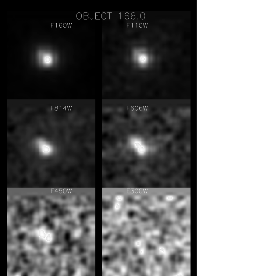
Figure 14: The image of NICMOS 166.0 in each of the six bands. All images have been stretched linearly so that the maximum flux is 1 and the minimum flux is 0. This hides the very large decline in flux with decreasing wavelength.

NICMOS 277.211 is in the region of the NICMOS 277.10 complex but is again clearly a separate galaxy. Its appearance is similar to NICMOS 166.0 with a single bright nucleus at 1.6 microns which decreases in intensity with decreasing wavelength. Low surface brightness structure is evident at the shorter wavelengths but unlike NICMOS 166.0 it does not disappear completely at 0.3 microns.

NICMOS 166.0 has a reasonably secure redshift determination with the $\chi^{2}$ value rising sharply for redshifts less than 1.66 so it is unlikely to be a low redshift and hence a low luminosity galaxy. There is a secondary minimum at higher redshift which would of course increase its luminosity. If the secondary minimum in the template extinction discussed in Section 6.3.1 is used the luminosity is decreased to $1.4\times 10^{11}$ L_⊙ which reduces it to LIRG status. NICMOS 277.211 has a secondary minimum in its $\chi^{2}$ distribution at a lower redshift of about 1.4. Reduction of its distance from a redshift 1.84 to 1.4 yields a luminosity of $4.4\times 10^{11}$ L_⊙ which would remove it from the ULIRG classification and demote it to the LIRG classification.

We also note that NICMOS 166.0 and 277.211 are coincident with the ISO sources PS3 17a and PS3 15 from Aussel et al. (1999). The observed flux levels at 15 $\micron$ are consistent with the fluxes predicted from our dust model. This is further evidence for these sources having significant extinctions.

Adelberger and Steidel (2000) give an empirical relation between the 850 $\micron$ flux and the 20 cm flux which is a function of redshift. With this relation and the predicted $850\micron$ fluxes from Table 1, the predicted 20 cm fluxes for NICMOS 166.0 and 277.211 are 30 and 19 micro Janskys. Comparison of the dust spectral energy distribution of Adelberger and Steidel (2000) and our distribution shows that our predicted $850\micron$ fluxes are roughly a factor of two below the Adelberger and Steidel (2000) fluxes. In fact the empirical function has very significant width which would allow the fluxes to vary by factors of two to three and still be within 1 $\sigma$ of the prediction. Muxlow et al. (2000) do not find any detections at the locations of the galaxies to a limit of 27 micro Janskys at 1.4 gigahertz. Radio maps very kindly provided by Dr. Muxlow in advance of publication show no contours for NICMOS 166.0 but some contours at the location of NICMOS 277.211 but still below their accepted lower limit.

If both of these objects are ULIRGs then their presence in one 50 arc second by 50 arc second field is surprising. The local space density of ULIRGs with luminosities of $10^{12}L_{\odot}$ is $8\times 10^{-8}$ Mpc^-3 Mag^-1 (Soifer et al. (1987)) which is roughly equal to the space density of quasars. At this density we would expect $1.5\times 10^{-4}$ ULIRGs in our redshift 2 bin. The presence of two ULIRGs in our field may indicate a much higher rate of merging and hence high luminosity galaxies at a redshift of 2 as suggested in some hierarchical galaxy formation models (eg Blain et al. 1999a ). Given all of these considerations we chose to designate these galaxies as possible ULIRGs.

The objects NICMOS 49.0, 102.0, and 277.212 have star formation rates of 69, 59, and 12 $M_{\odot}$ per year. The early classification of the SED for NICMOS 277.212, discussed in Section 7.2, puts it in a lower star formation rate category. All three of the galaxies are at the border of the LIRG luminosity classification with luminosities just over $10^{11}L_{\odot}$. Both NICMOS 49.0 and 102.0 have most of their luminosity reradiated as far infrared flux and can therefore be classified as LIRGS. NICMOS 277.212 has only 22$\%$ of its luminosity in the far IR and should be classified simply as a luminous galaxy. Our dust SED model predicts that NICMOS 49.0 should be an ISO source and it does correspond to the ISO source PM3 15 of Aussel et al. (1999).

8 Incompleteness Corrections to the Star Formation Rate History

We approach the correction to the measured star formation rate history due to galaxies which are too faint to be detected as well as to those portions of detected galaxies having surface brightness below our detection limit in two ways. The first, and traditional way integrates an assumed luminosity function to determine the contribution from unobserved objects, using the aperture corrections described in Section 2.1 to account for the outer lower surface brightness portions of galaxies. The second method uses the observed distribution of star formation intensity at low redshifts to correct for the unobserved portion of the distribution at high redshift.

8.1 Corrections Based on the Luminosity Function and Aperture Corrections

It is readily apparent by inspection of Figure 4 that at high redshifts we are sampling only part of the galaxy luminosity function. We can get an estimate of the possible error in our star formation rate by asking what portion of the total luminosity we are missing. The solid and dashed lines in Figure 4 represent the expected 0.6″ diameter aperture magnitudes for an L^∗ late type galaxy and an L^∗ early type galaxy respectively, (templates 5 and 1) with the assumptions described in section 4.1. The line for the late type L^∗ galaxy shows that it is easily detectable even at a redshift of 8. If the luminosity distribution of galaxies is represented by a Schechter function with a slope of $\alpha=-1.6$ then we can integrate the luminosity function for magnitudes fainter than our observed F160W AB magnitude limit of approximately 28.5 to estimate the missing luminosity assuming a given template type. Since most of the higher redshift galaxies are best represented by templates 5 or 6 we will use the template 5 line shown in the figure for the calculation. The fraction f of missing luminosity is

$$f=\frac{\Gamma(.4,L_{lim},\infty)}{\Gamma(.4,0.,\infty)}$$ (4)

$\Gamma$ is the incomplete gamma function and $L_{lim}$ is the ratio of $L/L^{*}$ represented by our estimated limiting F160W AB magnitude of 28.5. The results are given in the first column of Table 3. The table shows that up to a redshift of 6.0 the correction is less than 50% and is significantly less than that for lower redshifts. The leveling of the error and the shallow slope of the late L^∗ galaxy curve in Figure  4 is due to the redshift of the galaxy’s high UV flux into the F160W band.

Lanzetta et al 1999 have suggested that the value of L^∗ evolves with redshift z as $(1+z)^{-1.2}$ for redshifts greater than 2. If we recalculate the missing luminosity with the evolving value of L^∗ we get the second column in Table 3 which indicates that we are missing very substantial fractions of the luminosity at high redshifts. In fact by a redshift of 3.0 we are missing half of the luminosity. The boundary of the objects in Figure  4 is also well fit by a template 5 L^∗ galaxy with an extinction of E(B-V) = 0.2. The increasing extinction due to the decreasing rest wavelength of the F160W band mimics an evolving L^∗. At this point we do not have enough information to choose between the two effects.

There are also suggestions that the value of L^∗ may increase with redshift, at least to redshifts of 3 to 4. If that is the case the fraction of missing luminosity will be less than the first column of Table 3. In view of the uncertainty of the true form of the luminosity function we turn to a new method of correction described below.

8.2 Correction via the Surface Brightness Distribution Function

In view of the substantial uncertainties in both the aperture corrections and luminosity function corrections described above we have developed a new technique involving the star formation rate intensity distribution introduced by Lanzetta et al. (1999). This method calculates a star formation rate intensity for every pixel contained in an object. The star formation rate surface intensity x is defined as the star formation rate in solar masses per year in a pixel divided by the proper area of the pixel in kpc². A histogram of the distribution of the star formation rate surface density is then constructed by summing the proper areas of all pixels within a given star formation rate and redshift interval, divided by the star formation rate interval and the comoving volume. From this distribution function (denoted as h(x) by Lanzetta et al. (1999)) the star formation rate per comoving volume $\dot{\rho}$ for objects in a redshift bin is then given by

$$\dot{\rho}=\int_{0}^{\infty}xh(x)dx\ \mathrm{M_{\odot}\ year^{-1}\ Mpc^{-3}}$$ (5)

Following Lanzetta et al. (1999) Figure 15 plots h(x) for those galaxies in our list in each of our redshift bins. The left hand panel uses the extinction corrected star formation value while the right hand panel uses the uncorrected values. In each case we have fitted the distribution in the 0.5 to 1.5 redshift bin by a three point smoothed curve and overplotted this curve on the other redshift bins. The curve is adjusted by adding or subtracting a single value to the fitted log curve to match the bright end of the distribution for each redshift bin. Note that the solid curves in this figure are strictly empirical matches to the data, whereas the solid curves in the Lanzetta et al. (1999) plot represented the distribution expected from a bulge profile.

Figure 15: Plots of the star formation rate intensity distribution for the deep NICMOS HDF. The abscissa is the log of the star formation rate per unit area while the ordinate gives the distribution of this quantity per comoving volume in the redshift bin. The left hand panel is for star formation rates corrected for dust extinction, while for the right hand panel no extinction correction has been applied.

We next make the assumption that the shape of the extinction corrected h(x) distribution is the same at all redshifts and that we are successfully measuring the bright end of the distribution in all of the redshift bins. Although there is no theoretical basis for this assumption, the excellence of the fit in the lower redshift bins, each of which contains a completely independent set of objects and pixels, lends empirical support to the concept. Note that this is not an assumption on the sizes of galaxies at various epochs. Galaxies can be smaller (or bigger) at different epochs. As long as their cumulative distributions of surface brightness of star formation are similar the method is valid. Also note that we are not correcting individual galaxies but rather the total distribution of brightness of the ensemble of galaxies in a given redshift bin.

Under this assumption the deviation of the measured points below the empirical curve matched to the bright end of the distribution represents the missed star formation rate. We then recover the true total star formation rate by performing the integration given in equation  5, substituting the value of the empirical curve whenever the measured rate dips below the value given by the curve. Note that the value of the integral using the empirical curve reaches 59% of its final value by $x=-0.25$ and 94% of its final value by $x=-1.25$. We consider this new method a more robust measure of the missing star formation and consider its use applied to the extinction corrected distribution as our primary method of estimating the missing star formation rate. The last column of Table 3 shows the incompleteness corrections from this method when the extinction corrected distribution is used. Note that the corrections for this method fall generally between the extremes of the constant L^∗ corrections and the evolving L^∗ corrections.

The necessity of using the extinction corrected distribution rather than the uncorrected distribution can be seen by inspection of the right hand panel in Figure 15 where the distribution is again fitted to the curve in the 0.5 - 1.5 redshift bin. There is an inflection in the curve at high star formation rate intensities that we take to represent the dimming of high star formation regions due to extinction. The empirical curve is then a poorer match to the high star formation rate intensity distribution at higher redshifts where Figure 5 indicates that the extinction of the galaxies used in this study is considerably less. It is also important to use the highest possible spatial resolution to sample as much of the intensity distribution in each galaxy as possible.

It is important to verify the universality of our basic assumption that the distribution function is independent of redshift. It is desirable to do this using the highest possible spatial resolution of both UV and Optical as well as FIR images, in order to accurately determine the star formation rate independently for each small pixel. For a limited set of low redshift objects this is probably currently feasible but for higher redshift objects it will require NGST as well as the next generation of very large ground-based telescopes with high performance adaptive optics working at the shortest feasible wavelengths.

Table 4 gives the star formation rates derived at each level of correction for each of the methods discussed. The column labeled Uncorrected is the star formation rate that utilizes the zero extinction redshifts discussed in Section 3.4. Figure  16 shows what we consider to be the correct rates based on the empirical h(x) curve adjustment of the extinction corrected rates.

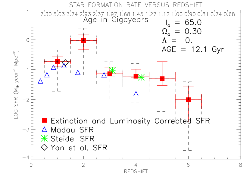
Figure 16: Plots of the extinction and incompleteness corrected star formation rate as a function of redshift. The solid error bars indicate the photometric errors and the dashed error bars indicate the uncertainty in the global star formation rate. The star formation rate from Yan et al. (1999) indicated by the diamond is for star formation in the range between a redshift of 0.8 to 2.0

9 Sub-millimeter and Far Infrared Flux

A constraint on the amount of extinction we have derived for both individual objects and for the entire field is the amount of far infrared flux produced. The 450 and 850 $\micron$ flux levels in the HDF have been measured by Hughes et al. (1998), and our predicted fluxes should not exceed these measured values, or the Hughes et al. (1998) et al upper limits on fluxes. In addition, Dwek et al. (1999) have determined that roughly half of the emitted flux from galaxies is absorbed and emitted as far infrared flux. Although the small size of our field allows deviation from this general result, as discussed in section 10, we should check to see if the total far infrared flux is similar to our observed fluxes in the optical and near infrared.

Our fits to template types and dust extinction enable us to calculate the ratio of the fluxes emitted in the optical and near infrared to that absorbed by dust and reradiated in the far infrared and sub-millimeter region. The observed 850 $\micron$ flux is then given by the assumed temperature distribution of the dust in the source and the redshift. Since we do not have any observational knowledge of the actual dust temperature distribution for our galaxies, we utilize the observed Arp 220 ULIRG spectrum given in figure 4 of Rowan-Robinson and Efstathiou (1993) as a standard dust spectral energy distribution. This model has a UV optical depth of 500 which converts essentially all of the optical and UV flux into far infrared flux. The integrated flux of this model is scaled to the luminosity removed by extinction for each galaxy. The model flux at the appropriate rest wavelength is then used to determine the expected 850 $\micron$ flux. It should be noted that variations in the actual dust SEDs from our model SED can easily introduce errors of factor of 2 to 3 in our calculated fluxes.

Table 1 gives the predicted 850 $\micron$ flux in milliJanskys. Inspection of the flux column in Table  1 shows that none of the source fluxes exceed the 2 milliJansky detection limit in the HDF set by Hughes et al. (1998) although three sources, NICMOS 49.0, 166.0, and 277.211 are quite close. Hughes et al. (1998) found no sources in our observed region of the Northern HDF, consistent with the Arp 220 model. This is not surprising since only five sources were detected in the Northern HDF and our area is 1/7 of the total area. Given the uncertainty of the fluxes we simply note that the predicted fluxes are consistent with the observations.

The ratio of the total power that is removed by extinction in all of the sources to the power that is not removed by extinction is 0.8, which implies roughly equal amounts of power in optical-UV background and the far infrared background. This is consistent with our current understanding of the distribution of background power as given by Dwek et al. (1999). This result comes strictly from our derived extinction and is not dependent on the assumed SED of the far infrared emission.

By summing all of the predicted 850 $\micron$ sources in our field we calculate a background surface brightness of $5.7\times 10^{-10}$ watts m^-2 sr^-1 for $\nu I(\nu)$ at 850 $\micron$ which compares to the measured values of $5\pm 2\times 10^{-10}$ (Blain et al. 1999b ) and $4\times 10^{-10}$ from COBE measurements (Fixsen et al. (1998)). Taken together, the rough equality of the optical-UV power and FIR-power noted above, together with the rough equality of the predicted and observed submillimeter fluxes suggests to us that i) a non-negligible fraction of star formation at all epochs and ii) A non-negligible portion of the submillimeter background is contributed by sources which are not the extremely super luminous sources represented by the SCUBA detections.

A similar number at 1.6 $\micron$ can be generated from the F160W source fluxes which is $6\times 10^{-9}$ watts m^-2 sr^-1 for $\nu I(\nu)$. This number is for detected discrete sources only. Gardner (1996) finds a lower limit on resolved sources from ground based surveys at 2.2 $\micron$ of $7.4\times 10^{-9}$ watts m^-2 sr^-1. Any confusion limited surface brightness from undetected sources will be removed by our background subtraction technique described in Thompson et al. (1999).

10 Sampling errors and Overall Error Estimates

In this section we make estimates of the uncertainties in our star formation rate determinations associated with the very small solid angle of our sample. We consider two approaches: 1) Analytic estimates 2) Utilization of numerical simulations.

10.1 Analytic Estimates

Conceptually, we distinguish between sampling errors arising from two different sources: a) Those arising from the fact that galaxies are spatially correlated (“large scale structure”) b) Those arising from the sampling of the luminosity function for the small numbers of galaxies, especially bright galaxies, in some of our bins.

10.1.1 Large Scale Structure

One effect of spatial clustering is to increase the variance in the number of objects in a cell over that expected from Poisson statistics. The fractional square root of the variance in the number of galaxies depends only upon the two-point correlation function and is given by Peebles (1980).

$$\sigma_{N}/N=\sqrt{1+N\times I_{2}}/\sqrt{N}$$ (6)

where

$$I_{2}={\int\int\xi(r_{o},\gamma)dV_{1}dV_{2}}/V^{2}$$ (7)

and where $\xi(r_{o},\gamma)$ is the two point correlation function. For each of our redshift bins it is a very good approximation to consider the volume to be a long thin tube of square cross section with sides of (comoving) dimension D and (comoving) length L. Then it is straightforward to show that the expression for $I_{2}$ has the form

$$I_{2}\simeq C(\gamma)\times(ro/D)^{\gamma}\times(D/L)$$ (8)

The quantity $L/D$ is simply the number of cubes of dimension $D\times D\times D$ that can be placed end to end in the tube of length L. The dimensionless coefficient $C(\gamma)$ is a double integral in which $dV_{1}$ is taken over the unit cube and $dV_{2}$ covers that same cube plus a large number of cubes on either side of this unit cube. We have evaluated this coefficient numerically which is vastly simplified by the large number of symmetries in this geometry. From the work of Adelberger et al. (1998) we adopt $\gamma$ = 1.8 and $ro=5h^{-1}$ Mpc. We find $C(\gamma=1.8)$ = 8.22. In Rows 1, 2, 3 and 4 of Table 5 we give the values of N, $1/\sqrt{N}$, I₂ and $\sigma_{N}/N$ computed from the above expressions for each of our six redshift bins. We use the value of D and L for our adopted cosmology appropriate to the center of each bin. For all bins except the last the term involving the two-point correlation dominates.

A difficulty with the application of equation (6) is that the simple description of galaxy clustering by means of a single luminosity-independent two-point correlation function is surely too simple. We have tried to mitigate this to some extent by using the correlation length derived by Adelberger et al. (1998) for the most luminous of the Ly-break galaxies. However, one can imagine an example in which each bright galaxy carries with it a fixed number of fainter galaxies. In this case the relevant value of N in equation (6) is the number of bright galaxies, not the total number in the cell, in which case we will underestimate the fractional variance.

10.1.2 Sampling Errors due to Small Numbers

Even in the absence of any statistical uncertainty in the number of objects in a given bin, there are sampling errors. As a qualitative indication of how important an effect this might be we show in Table 2 the percentage contribution to the total star formation rate in each bin from each of the most luminous objects. To obtain a quantitative estimate of the variance in the star formation rate we use the bootstrap resampling technique described in, e.g. Ling, Frenk and Barrow (1986) and the references therein. The fractional variance from this effect is shown in row 5 of Table 5. We assume that the total uncertainty due to sampling error is obtained by combining rows 4 and 5 in quadrature and the resulting fractional variation due to large scale structure and sampling error is given in row 6.

Obviously, if the global star formation rate is dominated by very rare and highly luminous objects which are not present in our sample at all we cannot take this into account. We return to this possibility in section 11.2.

Several groups have attempted to incorporate star formation into N-body/hydrodynamic simulations. This approach has the virtue that all the sampling issues discussed above can be automatically incorporated. Ideally these simulations should cover our full redshift range, have solid angles so large that all significant large scale structure is averaged out, should have adequate spatial resolution to represent objects of moderate galaxy masses, and of course, should actually model the star formation correctly. Such an ideal simulation would provide useful insights into both the role of large scale structure and the effects of sampling errors on data sets such as ours. Unfortunately no simulations that we are aware of combine both adequate scale with adequate resolution. However existing simulations can be used for other comparisons with our analysis, as discussed in section 11.2.

10.2 Overall Error Estimates

We have previously discussed two other sources of error in addition to the sampling errors just discussed: (i) Errors in the SFR resulting from photometric errors. An inspection of Figure 9 shows the 16% and 84% confidence limits determined as described in section 6.1 (which we take as indicative of $1\sigma$ errors) are in some cases quite asymmetric about the median and unperturbed values. We list these two upper and lower fractional errors in rows 7 and 8 of table 5. ii) Errors resulting from the high degree of degeneracy between stellar population type and internal reddening. These are over and above any errors in photometry and would arise from the failure of individual galaxies to be adequately represented by our set of 51 templates. Based upon the discussion of section 6.3.1 we estimated the fractional SFR error to be $\pm$ a factor of 2 in the SFR. For completeness we list these values in rows 9 and 10 of table 5. We do not include any error estimates for the accuracy of the incompleteness corrections. These corrections, based upon the histograms of Figure 14 are on the order of a factor of two at high redshift, as shown by table 4. The error in the correction should be significantly less than the correction which means it will be dominated by the sampling errors.

To get the total upper fractional error in the star formation rate we simply add the upper fractional errors in Table 4 in quadrature. If we also do this for the lower error the procedure leads to a negative star formation rate in some bins which is not physical. To compute the lower bound we simply multiplied the fractional lower errors in Table 4 together. This may be somewhat pessimistic since it assumes that all lower error fractions contribute their full weight to the fractional error. The calculated upper and lower errors are given in the last two rows of Table 4. These errors, when translated into SFR values, are plotted by the dashed error bars in Figure 16.

11 Discussion

In this section we compare our results with other studies and look at a few of the implications of our results. We do note that our measured star formation rate at a redshift of 5 is equal to that at redshift 3 thus satisfying the criterion for reionization by stars stated in Madau (1999) and discussed in the introduction. Of course this would require that a significant fraction of the Lyman continuum flux actually escape from these star forming galaxies, and it is exceedingly difficult to know if this is the case. As noted earlier, in our templates we have assumed that no Lyman continuum photons escape any of the galaxies.

11.1 Comparison with Other Optically-Derived Results

Except for a large discrepancy near a redshift of 2 our star formation rates in Figure 16 are roughly consistent with the rates found by Madau (1999). Our redshift 1 results are also consistent with H$\alpha$ derived rates of Yan et al. (1999) that cover the redshift range between 0.8 and 2.0 but our rate for a redshift of 2 is significantly higher than this due, as noted previously, to two very luminous reddened galaxies. The rates from a redshift of 3 through 5 are consistent with a constant star formation rate and agree with the values found by Steidel et al. (1999) based on data from a much larger area. All of the rates not based on our data have been adjusted to our cosmology. The solid line error bars on our results come from the techniques discussed in section 6. As such they represent the errors associated with the star formation rate in the NICMOS observed region of the Northern Hubble Deep Field. The dashed line error bars represent the errors in extrapolating this result to the universe in general taking account of other sources of error, including sampling errors (as discussed in section 10) in addition to the photometric error bars plotted in figure 6.

11.2 Comments on Other Star Formation History Work

We begin with a brief philosophical comment: As mentioned at the conclusion of Section 10.1.2, it is certainly conceivable that the average comoving density of star formation in any or all redshift bins is completely dominated by objects totally missing from our sample, either because they are very rare, and thus missing from our small solid angle survey, and/or because they are so heavily obscured that they are too faint to be seen even in our deep F110W and F160W images. Indeed, a current lively debate centers on just this latter possibility, as discussed further in Section 11.2.2.

While these possibilities and the global comoving star formation rate are obviously important issues, they are hardly the only issues. A complete picture of the history of star formation should, at the very least, encompass delineation of, and explanation for, a much more complex “star formation distribution function”, e.g. $\phi(SFR,fIR,z)$ giving the number of galaxies at redshift z undergoing star formation at a rate SFR with a fraction fIR of the luminosity being converted to the far infrared. Thus, despite our limited solid angle and the fact that the objects in our survey are near IR–selected we believe such surveys as this are of interest because they probe to low values of the SFR for objects which are not heavily obscured. We believe the deep NICMOS survey to be 50% complete at $m_{AB}F160W$ of 28.5 through an 0.6$\arcsec$ aperture. At a redshift of 3 a template fit of 5.5 and E(B-V) of 0.06, typical for our sample, the inferred star formation rate is 0.4 $M_{\odot}/yr$.

11.2.1 The Theoretical Model of Weinberg et al

Weinberg et al. (1999) present SPH numerical simulations to which they adjoin a recipe for star formation and energy deposition by supernovae. By combining models with different parameters they extend the resolution down to baryon masses of order $10^{8}$ (see their Table 1) and to star formation rates as low as 0.1 solar masses per year (see their Figure 1), though, as the authors point out, the flattening of the distribution at these low values may indicate they are resolution–limited at somewhat higher values.

We attempt a comparison between these models and our results as follows: (1) We restrict analysis to the objects for which we assigned redshifts in the range 2.5 to 4.5. In this range we are generally directly observing sufficiently far into the rest UV that we are less at the mercy of the template fitting than at lower redshifts, while at higher redshifts our sample is too small. (2) We omit objects for which the template fit is less than 4.0. In these cases we are looking at older populations where the bulk of the star formation has already taken place and where the SPH models may not apply. (3) The SFR is at least 0.5 at which point we may consider our sample to be fairly complete as suggested by the example above. We find 57 objects in Table 1 satisfying these criteria. We normalize the cumulative distribution of the number of objects as a function of their star formation rate for both our sample and the Weinberg et al. (1999) models. As noted above, for typical template and extinction values of the objects in this redshift range, we should be about 50% complete at a star formation rate of 0.4 $M_{\odot}/yr$. Thus, we normalize cumulative distributions defining them to be zero at the slightly higher value of 0.5 $M_{\odot}/yr$ and 1.0 at a star formation rate of $\infty$.

We may then compare the shapes of these distributions by examining the ratio of the star formation rates at the 25th percentile and 50th percentiles, and similarly at the 25th and 75th percentiles. We may also compare the absolute value of the star formation rate at the 25th percentile. Table 6 presents the result of these comparisons. Given the small number statistics of our sample and the errors discussed earlier this is rather remarkable agreement.

A difference does arise when we compare our actual observed surface density from this sample with the simulations. In our survey we find a surface density of 60 objects per square arc minute over this range. Adding together the number of objects in the redshift bins of 3 and 4 down to a SFR = 0.5 from Weinberg et al. (1999) their simulations predict a surface density of 400 objects per square arc minute, about seven times higher than we observe. Since their distribution is flattening at this point due to possible resolution effects, the discrepancy might be higher still.

It is not clear that this is a significant discrepancy. Our incompleteness corrections described in Section 8 correct for missed star formation not for the number of objects contributing to that rate. A small increase of 0.1 over our typical value of E(B-V) of 0.06 will result in more than a half magnitude of dimming at the rest wavelength of the F160W band in the redshift range from 3 to 4. Inspection of Figure 4 shows that this would remove a large number of faint sources from our view. Since the highest number of sources reside near the boundary of our detection limit it is difficult for the observations to accurately determine the absolute number.

Since the actual star formation rate is dominated by the brightest sources and the number statistics by the faintest sources, it is appropriate to compare our observations with the calculated star formation rates given in Figure 2 of Weinberg et al. (1999). The log of the star formation rate at redshifts of 3 to 4 in that figure is -0.5 while our value is a -1.1. Our “1 $\sigma$” error bar extends to -0.7 and of course the log of our star formation rate at a z of 2 is 0.0. There is a general trend of the numerical simulations to have somewhat higher star formation rates than we have observed but within the probable errors of both the simulations and the observation the gap is not wide.

11.2.2 SCUBA sources: Ly Break galaxies or an Optically Hidden Population

As indicated above, a lively debate is occurring between those who advocate that the bulk of the star formation at high redshift is occurring in luminous heavily obscured objects which can only be detected at submillimeter wavelengths and those who argue that optically–selected galaxies, even though subject to significant extinction, can account for both the bulk of the global star formation and indeed the bulk of the submillimeter flux as well. Our analysis in Section 9 favors the latter point of view. After that analysis had been completed we became aware of the work of Adelberger and Steidel (2000) who strongly favor this latter point of view, using a completely different sample and line of argument.

Adelberger and Steidel (2000) assemble data on narrow band fluxes and indices over a wide range of the electromagnetic spectrum from local sources to reconstruct typical SEDs of star forming galaxies and infer the shape of the dust emission and total star formation rate. They examine the correlations between these various pieces of data and examine the much more limited evidence at higher redshifts to see if these correlations hold. While the evidence is not overwhelming, a plausible case is made that they do, and in particular that the slope of the UV spectral index, $\beta$, is a good indicator of the submillimeter flux and along with the UV flux, can be used estimate the star formation rate.

As we have noted in Section 6, several combinations of extinctions and templates (and thus the total star formation rate and the fraction of energy converted to the far IR) produce very similar optical spectral energy distributions. Thus, as these authors themselves state, it is not clear why such a correlation should hold involving such complex situations as variable star formation histories, amount and geometry of dust obscuration etc. It is possible that the degeneracy which we explored in Section 6 could be broken as and when sufficiently large light gathering power is available to examine spectral features in the rest UV. Nevertheless, our estimates of the star formation rates in these high redshift bins agree well with those of Steidel et al. (1999), and the two independent conclusions on this issue seem to us to favor the point of view that observations in the optical and near infrared can determine the star formation rates accurately. With NICMOS we also easily observe sources which have more than $95\%$ of their luminosity being reemitted in the far infrared and whose 850 µm flux levels are below the SCUBA detection limit. Whether the rare, strong SCUBA sources are produced by objects which we could not detect in our F160W and F110W images will depend simply on whether the extinction to these sources is significantly greater than the amount needed to make most of their luminosity appear at far infrared wavelengths.

12 Conclusions

An important conclusion from our work is the relatively flat star formation rate between a redshift of 3 and 5 when corrections for both extinction and missed flux are taken into account. This implies that star formation occurs at a reasonably steady rate in the early universe. However it is still true that the vast majority of stars formed at redshifts less than 2 due to the much greater amount of time available at low redshift values. Explaining this behavior can provide a constraint to models of star and galaxy formation.

The ability of our observed sources to reasonably reproduce the observations of the net background at $850\micron$ indicates that the type of sources found in our study contribute significantly to the global star formation rate. Increases in the star formation rates by a factor of 10 due to extremely luminous objects represented by the SCUBA detections appears unlikely.

Our high star formation rate at z = 2 is due to the presence of two possible ULIRGs in our field which contribute 80 % of the measured star formation rate. The presence of two ULIRGs in our small field is highly unlikely at the local density of ULIRGs and it may imply a greatly increased number of merger events leading to high luminosity at a redshift of 2.

Table 1: Listing of measured quantities

NICMOS	WFPC	z	E(B-V)	SFR	Lum.	frac.	SCUBA	T	$\chi^{2}$	Tot.	Ap.	RA	DEC
ID	ID			M⊙	L⊙		850 µm			mag	mag	12$\fh$	+62$\fdg$
				yr-1			flux					36$\fm$
							mJy
1.00000	$\cdots$	1.52	0.00	0.356	7.06E+08	0.00	0.00	5.6	1.0	27.1	27.8	40.81	12:9.60
2.00000	4-830.0	3.84	0.10	2.710	7.53E+09	0.46	3.96E-03	5.5	2.0	27.0	27.2	40.96	12:10.8
502.000	4-807.0	3.84	0.00	1.146	3.21E+09	0.00	0.00	5.6	1.7	27.6	27.8	41.13	12:12.2
5.00000	4-822.0	0.16	0.70	0.615	1.28E+09	0.95	2.82E-02	6.0	2.6	24.7	25.2	41.14	12:10.6
10.0000	4-813.2	3.60	0.00	0.897	4.68E+09	0.00	0.00	4.8	0.6	26.8	26.9	41.42	12:6.80
11.0000	4-790.0	3.60	0.00	1.137	2.71E+09	0.00	0.00	6.0	0.2	27.7	27.9	41.43	12:11.4
14.0000	4-767.0	0.72	0.02	0.019	8.48E+09	0.02	6.26E-04	1.1	0.8	21.7	22.0	41.48	12:15.0
15.0000	4-813.0	3.36	0.00	2.917	8.97E+09	0.00	0.00	5.3	1.2	25.9	26.2	41.53	12:6.80
16.0000	4-794.0	0.80	0.10	0.432	1.15E+09	0.47	1.74E-03	5.6	0.4	26.1	26.5	41.55	12:8.10
1085.00	$\cdots$	0.48	0.20	-0.00	1.51E+08	0.60	$\cdots$	6.0	6.8	$\cdots$	$\cdots$	41.60	12:6.20
18.0000	$\cdots$	0.64	0.50	0.464	1.30E+09	0.92	2.60E-03	6.0	0.9	27.5	27.7	41.62	12:12.8
21.0000	4-739.0	0.32	0.50	0.243	5.42E+08	0.92	2.73E-03	6.0	0.3	26.9	27.3	41.64	12:16.1
1084.00	$\cdots$	3.36	0.00	3.595	1.34E+09	0.00	0.00	6.0	11.	28.4	30.7	41.66	12:6.40
26.1200	4-795.11	0.48	0.30	1.443	2.92E+09	0.77	1.24E-02	5.9	1.7	25.1	25.6	41.86	12:7.00
26.1000	4-795.0	0.40	0.10	0.460	7.12E+09	0.23	9.91E-03	3.0	2.5	20.8	21.4	41.94	12:5.40
1081.00	4-748.0	4.64	0.02	0.782	2.44E+09	0.12	3.42E-04	5.5	0.5	28.3	28.4	41.96	12:9.10
1086.00	$\cdots$	0.48	0.20	0.107	1.68E+08	0.56	6.98E-04	5.8	1.9	27.4	28.3	42.05	12:3.10
514.000	4-711.2	0.96	0.40	0.522	1.57E+09	0.88	2.34E-03	6.0	0.8	28.1	28.1	42.07	12:14.8
515.000	4-709.2	2.48	0.00	0.246	6.87E+08	0.00	0.00	5.5	2.5	27.9	28.2	42.15	12:13.8
27.0000	4-665.0	1.44	0.20	3.602	9.16E+09	0.60	8.95E-03	6.0	1.2	25.9	26.1	42.17	12:23.0
29.0000	4-769.0	0.96	0.20	1.362	3.07E+09	0.55	4.19E-03	5.7	1.7	25.7	26.2	42.29	12:1.40
31.0000	4-671.0	0.96	0.30	1.556	3.85E+09	0.75	6.34E-03	5.8	0.9	26.0	26.4	42.36	12:19.0
32.0000	4-690.0	1.12	0.40	2.459	5.39E+09	0.88	8.05E-03	6.0	1.5	26.5	26.9	42.37	12:13.9
33.0000	4-743.0	0.48	0.10	0.044	1.71E+08	0.50	2.58E-04	5.8	5.6	28.2	28.1	42.47	12:1.20
34.0000	4-715.0	4.00	0.08	1.626	4.44E+09	0.35	2.06E-03	5.2	0.3	27.4	27.8	42.54	12:5.60
35.0000	4-687.0	0.08	0.50	0.018	4.88E+07	0.92	3.23E-03	6.0	8.3	26.9	27.1	42.58	12:11.4
36.0000	4-619.0	2.96	0.10	1.219	4.44E+09	0.42	2.07E-03	5.3	0.4	26.9	27.0	42.61	12:25.3
1067.00	$\cdots$	3.92	0.00	1.417	1.68E+09	0.00	0.00	5.5	0.7	27.5	28.6	42.61	12:17.0
37.0000	4-725.0	1.84	0.00	0.661	2.16E+09	0.00	0.00	4.9	0.9	25.4	26.1	42.64	12:4.10
38.0000	4-636.0	0.64	0.40	1.675	4.15E+09	0.88	8.92E-03	6.0	1.5	25.9	26.2	42.65	12:20.9
43.0000	4-707.0	0.80	0.08	0.404	8.07E+08	0.43	1.38E-03	5.8	2.3	26.7	27.3	42.77	12:3.90
528.000	4-616.0	3.76	0.10	1.825	3.16E+09	0.47	2.74E-03	5.6	2.6	27.3	28.0	42.79	12:22.7
1071.00	4-655.0	2.72	0.00	0.422	9.99E+08	0.00	0.00	6.0	4.8	29.1	29.3	42.86	12:13.6
47.1000	4-581.0	1.92	0.10	6.356	1.51E+10	0.50	1.33E-02	5.8	2.3	25.0	25.3	42.87	12:27.8
45.0000	4-716.0	1.60	0.00	0.075	3.65E+08	0.00	0.00	5.4	0.6	28.6	28.4	42.88	12:0.00
46.0000	4-697.0	2.48	0.02	1.818	5.39E+09	0.12	1.16E-03	5.4	4.1	25.8	26.0	42.90	12:3.50
48.0000	4-606.0	2.80	0.20	2.997	5.49E+09	0.60	5.85E-03	6.0	0.1	27.2	27.7	42.91	12:22.8
49.0000	4-656.0	0.56	0.50	67.57	1.50E+11	0.91	4.99E-01	5.9	2.4	21.0	21.8	42.91	12:16.3
47.2000	4-581.2	1.84	0.02	1.502	4.31E+09	0.11	1.00E-03	5.3	1.8	25.4	25.8	42.96	12:26.6
51.0000	4-660.0	2.32	0.02	3.257	7.65E+09	0.13	1.28E-03	5.6	3.5	25.3	25.7	42.97	12:11.5
1073.00	4-649.0	1.12	0.02	0.094	2.29E+08	0.14	5.23E-05	5.9	2.9	28.7	29.1	43.09	12:11.2
54.0000	4-664.0	1.84	0.00	0.365	8.80E+08	0.00	0.00	5.5	3.6	27.1	27.6	43.11	12:7.20
56.0000	4-537.0	2.40	0.00	0.258	7.49E+08	0.00	0.00	5.2	8.4	27.2	27.7	43.12	12:31.0
57.0000	4-554.0	0.48	0.20	1.049	2.92E+09	0.53	6.92E-03	5.6	3.0	24.4	24.7	43.13	12:28.1
59.0000	4-599.0	2.80	0.00	2.622	7.78E+09	0.00	0.00	5.4	3.6	25.7	25.9	43.19	12:19.2
1062.00	4-600.0	4.48	0.00	1.725	2.46E+09	0.00	0.00	6.0	7.6	27.3	28.0	43.25	12:17.7
61.0000	4-590.0	2.08	0.30	21.32	4.89E+10	0.79	5.58E-02	6.0	1.1	24.8	25.1	43.30	12:18.3
1064.00	4-591.0	0.56	0.30	0.151	3.09E+08	0.77	9.51E-04	5.9	1.2	27.7	28.2	43.34	12:17.2
63.0000	4-605.0	2.80	0.00	0.629	2.41E+09	0.00	0.00	5.7	1.6	27.7	27.5	43.35	12:15.9
64.0000	4-677.0	0.32	0.20	0.080	1.69E+08	0.58	5.85E-04	5.9	2.5	27.2	27.8	43.40	12:1.00
1063.00	4-583.0	0.48	0.30	0.155	2.60E+08	0.79	1.32E-03	6.0	1.9	28.5	29.2	43.46	12:17.0
68.0000	4-565.0	0.56	0.40	21.52	4.71E+10	0.86	1.51E-01	5.9	1.4	22.5	23.0	43.62	12:18.3
70.0000	4-669.0	0.48	0.30	0.116	3.74E+08	0.79	9.97E-04	6.0	0.9	28.3	28.4	43.69	11:57.0
71.0000	4-572.0	0.48	0.30	1.051	1.97E+09	0.75	9.08E-03	5.8	1.1	25.1	25.8	43.70	12:15.6
72.0000	4-598.0	0.56	0.30	0.268	6.46E+08	0.75	1.70E-03	5.8	2.0	26.7	27.1	43.71	12:11.0
74.0000	4-513.0	1.04	0.20	0.266	6.82E+08	0.55	6.98E-04	5.7	1.3	27.7	28.0	43.75	12:25.2
554.000	4-492.0	4.16	0.02	0.362	2.24E+09	0.15	1.21E-04	6.0	0.3	29.4	28.6	43.79	12:29.1
75.0000	4-479.0	1.12	0.06	1.512	3.70E+09	0.35	2.12E-03	5.8	0.4	25.7	26.1	43.79	12:32.1
76.0000	4-525.0	0.56	0.10	0.141	6.85E+08	0.54	6.02E-04	6.0	1.9	28.0	27.6	43.81	12:22.4
77.0000	4-486.0	0.48	0.50	0.232	6.32E+08	0.92	2.32E-03	6.0	0.5	27.8	28.0	43.83	12:29.7
1072.00	4-595.0	2.40	0.06	0.426	7.14E+08	0.33	7.27E-04	5.6	1.6	27.8	28.6	43.86	12:8.00
562.000	4-663.0	4.88	0.06	0.925	2.27E+09	0.37	9.16E-04	6.0	3.1	28.8	28.9	43.91	11:54.4
79.0000	4-626.0	1.84	0.00	0.423	9.26E+08	0.00	0.00	5.8	0.6	27.6	28.0	43.91	12:2.20
81.1000	4-576.0	3.36	0.00	5.878	1.39E+10	0.00	0.00	5.5	1.1	25.4	25.8	44.02	12:9.50
80.0000	4-444.0	0.72	0.00	0.015	9.59E+07	0.00	0.00	4.2	0.8	27.1	27.5	44.02	12:36.5
1080.00	4-612.0	0.00	0.00	0.000	1.47E+02	0.00	0.00	4.4	0.4	27.8	28.4	44.03	12:3.00
83.0000	$\cdots$	1.12	0.00	0.074	2.84E+08	0.00	0.00	5.4	2.3	27.8	27.9	44.05	12:23.1
81.2000	4-576.2	1.52	0.20	2.869	6.61E+09	0.58	6.38E-03	5.9	0.5	26.0	26.3	44.07	12:9.20
86.0000	4-500.0	1.28	0.00	0.055	2.90E+08	0.00	0.00	5.2	1.4	27.9	27.8	44.08	12:23.4
87.0000	4-653.0	2.48	0.00	0.553	1.30E+09	0.00	0.00	5.6	4.4	27.2	27.6	44.10	11:53.3
1044.00	4-500.0	2.32	0.02	0.723	2.09E+09	0.15	2.85E-04	6.0	3.6	27.6	27.6	44.12	12:23.1
88.0000	4-430.0	0.72	0.06	0.870	2.58E+09	0.26	3.81E-03	5.0	3.5	23.5	24.3	44.19	12:40.4
1041.00	4-485.0	0.48	0.02	-0.00	8.56E+07	0.15	$\cdots$	6.0	1.3	$\cdots$	$\cdots$	44.23	12:23.1
568.000	4-577.0	3.92	0.10	1.160	2.93E+09	0.46	1.62E-03	5.5	0.3	28.1	28.4	44.26	12:4.60
1079.00	4-589.0	0.16	0.40	0.022	3.89E+07	0.88	9.39E-04	6.0	1.7	28.1	28.8	44.31	12:1.90
90.0000	4-580.0	1.04	0.30	0.603	1.26E+09	0.75	2.09E-03	5.8	0.7	27.2	27.7	44.33	12:3.20
91.0000	4-524.0	1.84	0.30	2.455	4.27E+09	0.79	8.27E-03	6.0	0.4	26.9	27.6	44.35	12:14.0
92.0000	4-499.0	4.88	0.20	5.781	1.37E+10	0.53	9.26E-03	5.6	7.9	27.4	27.7	44.44	12:17.2
571.000	4-534.0	0.96	0.40	0.658	1.29E+09	0.88	2.94E-03	6.0	2.5	27.9	28.5	44.46	12:9.80
94.0000	4-627.0	0.16	0.60	0.170	3.50E+08	0.95	7.82E-03	6.0	1.2	26.1	26.7	44.47	11:53.3
95.0000	4-438.0	1.12	0.06	0.327	9.53E+08	0.28	5.10E-04	5.2	0.0	26.0	26.5	44.49	12:30.5
96.0000	$\cdots$	4.88	0.20	6.143	1.15E+10	0.55	9.74E-03	5.7	1.7	27.4	27.9	44.54	12:36.1
97.0000	$\cdots$	1.28	0.60	18.83	3.57E+10	0.87	1.05E-01	5.5	3.2	23.6	24.3	44.56	12:15.4
98.0000	4-527.0	0.40	0.50	0.560	1.43E+09	0.92	8.03E-03	6.0	2.5	26.5	26.8	44.57	12:9.60
100.000	4-472.0	2.96	0.00	0.875	2.60E+09	0.00	0.00	5.2	1.2	26.7	27.1	44.59	12:20.4
579.000	4-546.0	1.28	0.20	0.447	1.03E+09	0.60	1.41E-03	6.0	0.0	28.0	28.4	44.62	12:4.20
101.000	4-632.0	0.24	0.06	0.000	8.47E+06	0.27	0.00	5.1	0.5	$\cdots$	29.0	44.62	11:48.8
1059.00	$\cdots$	1.68	0.30	1.232	1.91E+09	0.77	2.96E-03	5.9	2.7	27.5	28.3	44.63	12:14.0
102.000	4-445.0	1.84	0.30	80.45	1.74E+11	0.75	2.74E-01	5.8	3.6	22.8	23.3	44.64	12:27.4
103.000	4-625.0	4.48	0.10	21.19	5.47E+10	0.39	4.28E-02	5.1	0.5	24.8	25.4	44.66	11:50.5
1046.00	4-472.2	0.00	0.50	0.000	2.55E+03	0.91	0.00	5.9	0.7	27.4	28.2	44.67	12:20.4
584.000	$\cdots$	0.32	0.40	0.009	3.12E+07	0.69	1.42E-04	5.0	1.8	27.5	28.1	44.68	12:14.2
586.000	$\cdots$	5.68	0.06	2.998	5.02E+09	0.37	2.18E-03	6.0	0.0	27.5	28.0	44.71	12:20.0
107.000	$\cdots$	5.92	0.00	2.391	5.29E+09	0.00	0.00	5.2	0.0	27.1	27.7	44.72	12:18.8
109.000	4-579.0	0.48	0.20	1.103	3.00E+09	0.56	7.15E-03	5.8	0.8	24.9	25.2	44.74	11:57.1
110.000	4-603.0	2.56	0.02	2.072	4.88E+09	0.12	1.24E-03	5.4	1.9	25.7	26.2	44.74	11:54.4
1031.00	4-422.0	1.92	0.00	0.117	3.85E+08	0.00	0.00	5.4	2.0	28.1	28.3	44.77	12:29.3
588.000	4-483.0	0.96	0.08	0.102	2.84E+08	0.36	2.62E-04	5.3	0.2	27.3	27.8	44.79	12:14.5
114.000	4-558.0	0.48	0.40	5.404	1.01E+10	0.84	5.23E-02	5.8	4.3	23.3	24.0	44.83	12:0.20
116.000	4-509.0	1.12	0.00	0.020	3.52E+08	0.00	0.00	2.9	2.1	26.5	26.7	44.84	12:7.60
901.000	$\cdots$	1.20	0.30	4.297	1.10E+10	0.79	2.05E-02	6.0	1.8	25.7	25.9	44.89	12:40.1
118.000	4-601.0	6.56	0.00	2.201	4.85E+09	0.00	0.00	6.0	1.3	27.5	27.7	44.90	11:50.3
117.000	4-455.0	1.76	0.10	1.379	3.56E+09	0.49	3.48E-03	5.7	1.6	26.5	26.8	44.90	12:19.3
119.000	4-351.0	2.48	0.02	0.626	2.09E+09	0.11	4.26E-04	5.2	2.1	26.6	26.9	44.93	12:42.7
120.000	4-423.0	1.76	0.40	9.998	2.11E+10	0.84	4.18E-02	5.8	2.4	25.4	25.9	44.95	12:26.6
592.000	4-458.0	4.00	0.10	3.114	5.40E+09	0.49	4.09E-03	5.7	1.4	27.3	28.0	44.95	12:17.7
123.000	4-607.0	1.04	0.50	0.618	1.67E+09	0.92	2.47E-03	6.0	0.1	28.1	28.3	44.96	11:48.8
124.000	$\cdots$	1.12	0.02	0.499	2.62E+09	0.07	4.55E-04	3.8	0.5	24.0	24.8	44.99	12:39.7
125.000	4-596.0	0.48	0.04	0.126	3.41E+08	0.23	3.76E-04	5.6	2.2	26.5	26.9	45.03	11:49.4
126.000	4-515.0	3.44	0.10	0.994	2.78E+09	0.50	1.77E-03	5.8	1.1	28.1	28.2	45.04	12:3.00
127.000	4-543.0	1.28	0.20	5.356	1.07E+10	0.60	1.69E-02	6.0	2.4	25.2	25.7	45.05	11:58.1
141.120	4-571.0	0.72	0.08	0.503	1.59E+09	0.32	2.75E-03	5.0	3.2	24.1	24.8	45.06	11:54.2
128.000	4-431.2	2.88	0.00	0.211	1.23E+09	0.00	0.00	4.2	1.6	27.3	27.7	45.08	12:22.1
1075.00	4-526.0	4.72	0.02	0.750	1.82E+09	0.14	3.13E-04	5.9	1.7	28.6	28.8	45.11	12:0.40
130.000	4-573.0	2.88	0.00	0.300	2.42E+09	0.00	0.00	3.8	3.3	26.7	26.9	45.14	11:50.3
1022.00	$\cdots$	1.12	0.10	0.603	1.49E+09	0.47	1.23E-03	5.6	1.2	26.4	26.8	45.14	12:39.4
131.000	4-530.0	4.56	0.00	1.700	3.66E+09	0.00	0.00	6.0	3.0	27.5	27.8	45.15	11:59.7
132.000	$\cdots$	2.00	0.10	7.019	1.23E+10	0.50	1.35E-02	5.8	3.1	24.9	25.6	45.15	12:5.50
133.000	4-329.0	2.88	0.00	1.660	5.41E+09	0.00	0.00	5.3	2.1	26.1	26.3	45.17	12:44.5
1055.00	$\cdots$	2.72	0.00	0.373	9.18E+08	0.00	0.00	6.0	1.6	28.8	29.0	45.22	12:12.5
135.000	4-407.0	0.56	0.40	2.548	5.26E+09	0.88	1.77E-02	6.0	1.4	25.2	25.7	45.27	12:25.7
136.000	$\cdots$	0.40	0.50	0.781	1.93E+09	0.92	1.12E-02	6.0	2.1	26.1	26.5	45.27	11:45.4
141.112	4-555.11	2.96	0.10	30.17	6.34E+10	0.46	4.86E-02	5.5	3.3	23.7	24.3	45.28	11:52.2
137.000	4-342.0	0.56	0.08	0.196	6.16E+08	0.45	7.21E-04	5.9	3.2	27.3	27.4	45.31	12:38.6
138.000	4-498.0	1.92	0.10	1.694	4.99E+09	0.46	3.66E-03	5.5	1.7	25.9	26.2	45.32	12:3.50
141.111	4-555.0	0.80	0.00	0.040	1.06E+10	0.00	0.00	1.2	0.7	21.6	22.0	45.33	11:54.5
139.000	4-395.0	0.72	0.20	1.285	2.99E+09	0.60	7.01E-03	6.0	3.8	26.3	26.7	45.35	12:26.8
140.000	4-368.0	1.92	0.30	17.11	3.69E+10	0.73	5.40E-02	5.7	0.4	24.4	24.9	45.36	12:33.7
142.000	4-379.0	4.32	0.00	1.277	2.18E+09	0.00	0.00	6.0	1.9	28.4	29.0	45.37	12:31.0
604.000	4-559.2	2.64	0.00	0.535	1.03E+09	0.00	0.00	5.9	0.0	28.0	28.5	45.39	11:47.7
141.112	4-555.1	3.12	0.00	15.28	5.85E+10	0.00	0.00	4.8	3.8	23.2	23.7	45.41	11:53.2
146.000	4-467.0	3.20	0.04	0.530	1.56E+09	0.24	3.59E-04	5.7	2.8	28.2	28.3	45.42	12:7.80
148.000	4-557.0	2.16	0.00	1.365	8.43E+09	0.00	0.00	4.2	0.4	24.6	24.9	45.42	11:49.0
150.000	$\cdots$	4.80	0.20	10.22	1.70E+10	0.60	1.66E-02	6.0	2.1	26.9	27.5	45.42	12:2.20
147.000	4-384.2	1.68	0.00	0.158	4.55E+08	0.00	0.00	5.2	0.4	27.4	27.9	45.43	12:28.3
149.000	4-330.0	0.96	0.10	0.304	6.29E+08	0.50	8.35E-04	5.8	2.0	27.4	28.0	45.44	12:39.6
1077.00	4-507.0	3.68	0.00	0.000	6.55E+08	0.00	0.00	6.0	4.1	$\cdots$	29.9	45.48	11:57.3
607.000	4-397.0	3.20	0.30	4.452	8.46E+09	0.77	8.76E-03	5.9	1.1	27.4	27.8	45.49	12:23.6
153.000	4-424.0	0.56	0.50	0.161	4.57E+08	0.91	1.19E-03	5.9	0.7	27.9	28.1	45.50	12:16.5
154.000	4-487.0	1.92	0.02	0.663	1.74E+09	0.15	3.86E-04	6.0	3.9	27.5	27.6	45.50	12:2.10
155.000	4-344.0	1.20	0.20	1.659	3.63E+09	0.58	5.99E-03	5.9	1.1	26.3	26.7	45.51	12:34.6
159.000	4-345.0	1.36	0.20	1.870	4.84E+09	0.56	5.24E-03	5.8	2.3	26.1	26.4	45.57	12:33.6
163.000	4-389.0	2.72	0.08	4.874	1.04E+10	0.42	7.86E-03	5.7	0.4	25.8	26.3	45.62	12:25.0
165.000	4-563.0	4.40	0.06	2.847	2.28E+10	0.17	6.89E-03	3.4	0.0	26.0	26.4	45.64	11:43.1
167.000	4-551.0	4.00	0.00	1.435	2.68E+09	0.00	0.00	6.0	2.8	27.8	28.3	45.65	11:45.8
166.000	4-307.0	1.60	1.00	534.7	1.21E+12	0.97	1.78E+00	5.9	0.6	22.5	22.9	45.66	12:42.0
141.200	4-516.0	1.04	0.10	1.329	8.95E+09	0.31	5.10E-03	4.1	0.8	23.2	23.6	45.66	11:54.0
170.000	$\cdots$	0.32	0.50	0.028	6.78E+07	0.81	3.84E-04	5.3	0.1	27.1	27.8	45.73	12:27.1
171.000	4-323.0	2.80	0.00	0.295	1.04E+09	0.00	0.00	5.6	3.1	28.3	28.2	45.73	12:35.9
172.000	4-497.0	2.88	0.00	4.303	1.16E+10	0.00	0.00	5.4	2.3	25.2	25.6	45.74	11:57.3
174.000	4-478.0	2.64	0.10	0.487	1.74E+09	0.47	9.80E-04	5.6	0.1	28.2	28.1	45.77	11:59.1
177.000	4-520.0	0.00	0.00	0.000	2.15E+03	0.00	0.00	4.4	1.3	25.1	25.4	45.79	11:50.6
175.000	4-419.0	1.92	0.20	1.719	3.65E+09	0.60	4.02E-03	6.0	2.8	27.0	27.4	45.79	12:13.7
176.000	4-387.0	0.56	0.30	0.374	8.69E+08	0.77	2.36E-03	5.9	2.0	26.7	27.2	45.80	12:22.5
1066.00	4-464.0	0.56	0.02	0.040	1.24E+08	0.14	4.74E-05	5.8	1.9	28.4	28.5	45.84	12:1.10
184.000	4-473.0	5.52	0.00	4.507	9.08E+09	0.00	0.00	6.0	0.4	26.6	26.9	45.88	11:58.2
625.000	4-441.0	3.20	0.20	1.227	3.14E+09	0.58	1.82E-03	5.9	1.1	28.3	28.4	45.91	12:5.60
1049.00	4-414.0	0.16	0.10	0.009	1.73E+07	0.54	2.47E-04	6.0	1.4	29.4	30.1	45.92	12:12.7
1029.00	4-343.0	0.48	0.50	0.382	4.15E+08	0.92	3.81E-03	6.0	0.8	27.4	28.6	45.92	12:27.9
188.000	4-514.0	1.20	0.08	1.490	3.71E+09	0.43	4.16E-03	5.8	1.2	25.8	26.2	45.94	11:49.5
187.000	4-326.0	1.92	0.10	1.005	2.93E+09	0.50	2.11E-03	5.8	1.3	26.9	27.0	45.95	12:31.5
186.000	4-305.0	0.96	0.40	4.937	1.03E+10	0.88	2.21E-02	6.0	5.4	25.4	25.9	45.95	12:38.3
189.000	4-460.0	0.56	0.40	7.682	1.54E+10	0.86	5.39E-02	5.9	1.5	23.6	24.2	45.96	12:1.40
190.000	4-391.0	0.08	0.08	0.000	5.79E+06	0.45	0.00	5.9	2.8	$\cdots$	28.7	46.01	12:17.7
191.000	4-353.0	2.64	0.06	1.700	3.58E+09	0.35	2.36E-03	5.8	0.2	26.9	27.4	46.04	12:23.8
193.000	$\cdots$	1.68	0.02	0.077	4.04E+08	0.07	5.42E-05	4.0	5.8	27.3	27.9	46.09	12:26.7
628.000	4-293.0	0.96	0.40	1.173	1.76E+09	0.88	5.25E-03	6.0	0.1	27.1	28.0	46.10	12:36.6
195.000	4-331.0	3.36	0.02	1.433	2.71E+09	0.12	7.60E-04	5.4	0.6	26.9	27.6	46.14	12:27.4
198.200	4-522.0	1.12	0.30	7.191	1.54E+10	0.79	2.12E-02	6.0	2.6	25.0	25.5	46.15	11:45.0
197.000	4-299.0	4.24	0.02	1.400	3.67E+09	0.11	4.72E-04	5.3	1.9	27.3	27.7	46.16	12:34.6
196.000	4-285.0	2.16	0.20	0.877	2.52E+09	0.48	1.76E-03	5.3	1.1	26.8	27.2	46.17	12:36.8
632.000	4-396.2	3.20	0.20	1.538	3.02E+09	0.58	2.28E-03	5.9	1.9	28.0	28.4	46.17	12:12.4
198.100	$\cdots$	1.04	0.08	1.250	2.40E+10	0.17	7.67E-03	2.7	1.4	21.2	21.9	46.18	11:42.1
633.000	4-362.0	0.48	0.30	0.199	4.34E+08	0.79	1.71E-03	6.0	1.9	27.9	28.3	46.19	12:20.3
200.000	4-465.0	0.48	0.50	0.158	3.94E+08	0.92	1.57E-03	6.0	1.1	28.3	28.6	46.20	11:55.2
199.000	4-294.0	3.76	0.08	1.979	4.31E+09	0.38	2.65E-03	5.4	1.9	27.1	27.6	46.21	12:35.2
201.100	4-322.0	1.68	0.30	23.32	5.57E+10	0.75	5.64E-02	5.8	3.1	24.0	24.3	46.21	12:28.4
201.000	$\cdots$	0.00	0.00	0.000	2.69E+03	0.00	0.00	4.1	2.9	24.3	24.9	46.23	12:29.1
204.000	4-448.0	0.48	0.50	3.561	6.00E+09	0.92	3.55E-02	6.0	4.4	24.7	25.4	46.27	11:59.8
203.000	4-341.0	3.36	0.08	1.558	4.24E+09	0.42	2.52E-03	5.7	0.3	27.4	27.6	46.27	12:22.8
202.000	4-300.0	0.56	0.30	1.424	3.60E+09	0.73	9.14E-03	5.7	3.3	24.7	25.1	46.27	12:33.5
207.000	4-327.0	1.84	0.30	9.414	2.03E+10	0.79	3.17E-02	6.0	0.5	25.5	25.9	46.36	12:24.8
640.000	4-390.0	1.76	0.20	0.907	1.55E+09	0.60	2.54E-03	6.0	0.7	27.9	28.5	46.37	12:11.6
208.000	4-372.0	0.48	0.50	0.987	2.20E+09	0.92	9.83E-03	6.0	2.1	26.2	26.6	46.39	12:15.8
209.000	$\cdots$	0.88	0.02	0.548	1.17E+09	0.11	5.41E-04	5.2	0.2	24.9	25.8	46.41	12:4.60
210.000	4-489.0	1.84	0.08	0.564	1.53E+09	0.41	1.13E-03	5.6	1.6	27.1	27.4	46.42	11:46.5
647.000	4-443.0	1.76	0.10	0.329	7.42E+08	0.46	8.52E-04	5.5	1.4	27.6	28.2	46.45	11:56.3
645.000	4-262.2	5.52	0.00	1.483	3.61E+09	0.00	0.00	6.0	2.7	28.1	28.2	46.45	12:37.5
211.000	4-303.0	1.92	0.30	1.606	4.02E+09	0.69	5.26E-03	5.5	2.4	26.6	27.0	46.49	12:27.9
212.000	4-471.0	0.32	0.00	0.009	2.74E+09	0.00	0.00	1.2	6.5	21.2	21.5	46.51	11:51.4
213.000	4-488.0	2.48	0.02	3.169	7.48E+09	0.14	1.97E-03	5.9	5.1	25.8	26.1	46.53	11:45.6
1054.00	$\cdots$	0.48	0.40	0.065	1.88E+08	0.86	6.29E-04	5.9	0.7	28.5	28.6	46.54	12:6.10
214.000	4-416.0	0.48	0.30	3.081	7.30E+09	0.77	2.64E-02	5.9	1.7	24.2	24.6	46.55	12:3.10
216.000	4-434.0	0.16	0.40	0.227	5.36E+08	0.88	9.67E-03	6.0	3.1	25.5	25.9	46.58	11:57.2
215.000	4-350.0	1.20	0.00	0.079	6.38E+08	0.00	0.00	3.8	1.2	26.2	26.5	46.59	12:15.5
218.000	4-412.0	3.20	0.06	0.946	2.18E+09	0.32	9.02E-04	5.5	2.6	27.5	27.9	46.60	12:1.90
220.000	4-475.0	3.68	0.02	3.183	8.01E+09	0.12	1.40E-03	5.4	4.4	26.2	26.6	46.65	11:46.3
219.000	4-280.0	3.84	0.02	2.027	5.61E+09	0.15	7.98E-04	6.0	8.3	27.2	27.2	46.67	12:30.1
221.000	4-411.0	0.16	0.02	0.004	2.99E+07	0.14	3.35E-05	5.8	1.4	28.8	28.2	46.67	12:0.80
222.000	4-442.0	0.64	0.10	0.232	9.41E+08	0.38	9.93E-04	5.0	0.6	24.8	25.2	46.67	11:54.0
652.000	4-388.0	2.88	0.02	0.760	1.61E+09	0.13	3.47E-04	5.7	1.3	27.5	28.0	46.69	12:7.10
225.000	4-336.0	2.32	0.02	0.786	2.40E+09	0.11	3.37E-04	5.2	3.1	26.2	26.6	46.73	12:16.1
226.000	4-334.0	0.48	0.50	0.709	1.82E+09	0.92	7.07E-03	6.0	5.2	26.6	26.9	46.73	12:17.6
228.000	4-388.2	2.96	0.04	0.472	1.48E+09	0.19	4.36E-04	5.1	0.0	27.4	27.8	46.77	12:6.80
230.000	4-432.0	0.48	0.30	0.183	4.27E+08	0.75	1.58E-03	5.8	1.3	26.9	27.3	46.80	11:53.7
1018.00	$\cdots$	0.32	0.40	0.015	3.83E+07	0.71	2.13E-04	5.1	3.3	27.2	28.1	46.80	12:34.8
231.000	4-382.2	2.88	0.04	0.924	2.42E+09	0.22	8.02E-04	5.4	1.3	27.1	27.4	46.81	12:5.80
232.000	4-360.0	0.00	0.00	0.000	2.50E+02	0.00	0.00	4.7	0.8	28.0	28.1	46.82	12:9.40
235.000	4-289.0	2.88	0.00	6.719	1.53E+10	0.00	0.00	5.7	1.6	25.1	25.5	46.93	12:26.1
236.000	4-295.0	1.12	0.30	1.636	3.94E+09	0.79	4.82E-03	6.0	6.6	26.7	27.0	46.94	12:23.1
237.000	4-382.0	0.08	0.60	0.269	5.45E+08	0.95	4.91E-02	6.0	5.5	24.2	24.8	46.95	12:5.40
1027.00	4-295.2	0.96	0.30	0.778	1.62E+09	0.79	3.14E-03	6.0	1.1	27.3	27.8	46.96	12:23.4
238.000	4-415.0	0.48	0.20	0.460	1.08E+09	0.56	2.99E-03	5.8	2.9	25.8	26.3	47.00	11:56.3
1026.00	4-266.0	0.48	0.20	0.130	2.62E+08	0.60	8.44E-04	6.0	2.3	28.1	28.6	47.02	12:26.8
240.000	4-332.0	0.48	0.20	1.440	3.34E+09	0.58	9.31E-03	5.9	0.9	25.0	25.4	47.08	12:12.5
662.000	$\cdots$	0.24	0.70	0.005	1.96E+07	0.80	1.68E-04	5.0	0.1	27.7	28.2	47.14	12:0.60
663.000	4-216.2	3.92	0.00	1.496	2.38E+09	0.00	0.00	6.0	3.2	27.8	28.4	47.18	12:33.1
241.000	4-335.0	0.56	0.20	0.371	7.86E+08	0.60	1.76E-03	6.0	1.4	27.1	27.6	47.22	12:8.60
242.000	4-332.2	0.56	0.10	0.546	1.52E+09	0.52	2.32E-03	5.9	1.5	26.2	26.4	47.23	12:12.6
243.000	4-385.0	0.16	0.40	0.167	3.86E+08	0.88	7.12E-03	6.0	2.7	25.9	26.3	47.23	11:59.0
1050.00	$\cdots$	1.84	0.02	0.106	2.99E+08	0.11	7.36E-05	5.2	4.1	28.0	28.5	47.23	12:5.10
244.000	4-232.0	0.40	0.40	7.773	1.54E+10	0.86	1.07E-01	5.9	3.5	23.0	23.6	47.29	12:30.7
244.200	4-232.2	0.48	0.30	0.395	9.33E+08	0.75	3.41E-03	5.8	2.9	26.1	26.6	47.33	12:29.0
245.000	4-298.0	2.64	0.04	1.804	4.24E+09	0.27	1.82E-03	6.0	6.9	27.1	27.3	47.34	12:15.8
246.000	4-356.0	1.12	0.06	0.274	8.01E+08	0.32	3.93E-04	5.5	0.3	26.9	27.2	47.41	12:0.60
247.000	4-319.0	0.72	0.40	1.988	4.32E+09	0.88	1.59E-02	6.0	3.2	26.0	26.4	47.46	12:8.40
248.000	$\cdots$	5.76	0.00	2.331	5.37E+09	0.00	0.00	5.3	0.3	27.2	27.7	47.46	11:59.9
249.000	4-315.0	1.76	0.00	1.824	5.11E+09	0.00	0.00	5.2	1.9	24.9	25.4	47.48	12:11.2
250.000	4-291.0	0.96	0.60	1.686	4.51E+09	0.95	8.12E-03	6.0	1.9	27.0	27.2	47.51	12:14.1
251.000	4-346.0	0.72	0.04	0.396	1.39E+09	0.18	1.24E-03	5.0	8.3	24.3	24.9	47.51	12:2.60
1092.00	$\cdots$	0.48	0.50	0.132	4.13E+08	0.92	1.32E-03	6.0	1.4	28.4	28.4	47.64	12:31.6
255.000	4-301.2	1.36	0.00	0.255	4.67E+08	0.00	0.00	5.6	1.2	27.4	28.1	47.66	12:8.90
256.000	4-283.0	2.88	0.00	0.717	2.38E+09	0.00	0.00	5.6	6.1	27.3	27.3	47.67	12:12.5
257.000	4-231.0	0.64	0.10	0.076	2.19E+08	0.44	2.62E-04	5.4	0.6	27.0	27.4	47.67	12:22.1
258.000	4-308.0	2.16	0.00	0.642	1.69E+09	0.00	0.00	5.5	3.4	26.7	27.1	47.67	12:8.20
259.000	4-247.0	0.40	0.00	0.019	6.83E+07	0.00	0.00	5.5	2.5	28.1	28.2	47.69	12:19.3
260.000	$\cdots$	0.08	1.00	0.000	3.51E+06	0.88	1.74E-04	5.0	0.6	28.1	28.1	47.81	12:11.0
261.000	4-212.0	1.12	0.06	0.963	2.38E+09	0.33	1.36E-03	5.6	0.2	25.7	26.2	47.82	12:24.2
1040.00	$\cdots$	5.44	0.00	1.374	2.16E+09	0.00	0.00	6.0	0.7	28.1	28.7	47.83	12:4.50
264.000	4-304.0	0.72	0.50	1.385	3.68E+09	0.91	1.18E-02	5.9	1.1	26.1	26.3	47.86	12:5.40
265.000	4-174.0	0.00	0.20	0.000	7.24E+02	0.43	0.00	5.0	0.3	27.4	27.5	47.89	12:29.5
680.000	$\cdots$	0.00	0.00	0.000	3.18E+02	0.00	0.00	5.4	0.9	29.2	29.0	47.91	12:18.5
267.000	4-314.0	4.80	0.00	2.280	4.97E+09	0.00	0.00	6.0	0.7	27.3	27.5	48.00	12:0.80
1025.00	4-198.0	0.96	0.04	0.000	2.53E+08	0.27	0.00	6.0	2.7	$\cdots$	30.8	48.06	12:22.5
277.120	4-260.0	0.56	0.30	3.895	8.90E+09	0.77	2.45E-02	5.9	2.7	24.2	24.6	48.12	12:14.9
269.000	4-265.0	0.00	0.40	0.000	9.87E+02	0.82	0.00	5.7	1.0	28.3	28.6	48.15	12:8.40
277.100	4-260.11	0.88	0.00	0.392	2.90E+09	0.00	0.00	3.2	0.4	23.1	23.9	48.25	12:13.9
273.000	4-170.0	0.48	0.30	0.114	3.17E+08	0.77	9.85E-04	5.9	2.1	27.7	27.9	48.31	12:22.8
685.000	4-158.0	3.52	0.06	0.798	1.86E+09	0.35	9.48E-04	5.8	4.0	28.1	28.3	48.35	12:23.9
274.000	4-200.0	4.72	0.04	5.725	1.50E+10	0.20	4.83E-03	5.2	9.7	26.0	26.5	48.37	12:17.3
275.000	4-237.0	0.96	0.20	0.401	1.02E+09	0.58	1.22E-03	5.9	1.9	27.5	27.8	48.41	12:9.00
276.000	4-135.0	0.08	0.70	0.016	4.68E+07	0.95	2.93E-03	6.0	0.6	27.4	27.5	48.43	12:27.0
278.000	4-228.0	1.68	0.10	0.253	7.02E+08	0.49	4.14E-04	5.7	1.3	28.2	28.4	48.50	12:8.40
279.000	$\cdots$	1.36	0.20	1.910	3.98E+09	0.58	5.33E-03	5.9	3.3	26.3	26.8	48.57	12:27.0
280.000	4-257.0	0.56	0.20	0.701	1.98E+09	0.53	3.40E-03	5.6	3.8	25.0	25.4	48.58	12:3.90
281.000	4-229.0	0.80	0.20	1.190	3.29E+09	0.55	5.30E-03	5.7	2.0	25.4	25.7	48.62	12:7.80
277.211	4-186.0	1.84	0.70	375.2	1.07E+12	0.95	1.51E+00	6.0	2.8	22.4	22.9	48.62	12:15.8
277.220	4-260.2	0.48	0.20	0.746	1.62E+09	0.51	5.00E-03	5.5	1.7	24.5	25.1	48.65	12:14.2
282.000	4-111.0	0.00	0.20	0.000	7.02E+02	0.49	0.00	5.4	10.	28.8	28.7	48.67	12:26.3
277.212	4-169.0	5.04	0.08	16.84	1.19E+11	0.22	3.74E-02	3.5	0.0	24.6	25.1	48.71	12:16.7
1023.00	4-143.0	2.64	0.00	-0.00	4.74E+08	0.00	$\cdots$	6.0	3.8	$\cdots$	$\cdots$	48.74	12:20.5
283.000	4-154.0	0.48	0.40	0.815	1.91E+09	0.84	7.88E-03	5.8	6.8	25.4	25.8	48.75	12:19.1
690.000	4-203.2	1.52	0.10	0.590	1.08E+09	0.52	1.18E-03	5.9	1.6	27.6	28.2	48.82	12:8.40
284.000	4-183.0	0.32	0.30	0.003	2.18E+07	0.55	5.49E-05	4.6	0.2	27.8	28.0	48.84	12:12.0
693.000	$\cdots$	4.88	0.00	1.045	2.04E+09	0.00	0.00	6.0	0.2	28.2	28.6	48.86	12:16.8
285.000	4-128.0	1.92	0.10	1.019	1.91E+09	0.54	2.14E-03	6.0	3.5	27.2	27.7	48.88	12:20.2
286.000	4-199.0	0.00	0.08	0.000	3.08E+02	0.25	0.00	4.0	0.7	26.9	27.4	48.89	12:8.70
288.100	4-203.0	0.48	0.50	2.006	4.64E+09	0.92	2.00E-02	6.0	1.5	25.4	25.7	48.91	12:8.00
287.000	4-148.0	4.64	0.00	1.558	2.31E+09	0.00	0.00	6.0	1.5	27.9	28.6	48.92	12:16.7
1019.00	4-105.0	2.16	0.00	0.279	5.38E+08	0.00	0.00	5.9	0.2	28.3	28.8	48.97	12:23.2
288.200	4-203.12	2.80	0.02	0.790	2.88E+09	0.10	4.41E-04	5.1	3.7	26.5	26.8	49.01	12:8.20
289.000	$\cdots$	0.72	0.08	1.699	7.07E+09	0.32	9.29E-03	5.0	2.0	22.4	23.2	49.06	12:21.3
696.000	4-124.0	0.32	0.00	0.003	1.47E+07	0.00	0.00	5.0	2.9	28.5	28.9	49.18	12:16.1
290.000	4-99.0	0.56	0.08	0.111	2.76E+08	0.43	4.11E-04	5.8	4.4	27.5	27.8	49.28	12:20.0
292.000	4-131.0	0.72	0.30	3.471	7.08E+09	0.77	2.51E-02	5.9	2.1	24.8	25.3	49.33	12:14.5
293.000	$\cdots$	2.64	0.10	2.307	4.71E+09	0.47	4.64E-03	5.6	3.0	26.5	27.1	49.47	12:22.5
294.000	4-119.0	0.80	0.00	0.129	3.46E+08	0.00	0.00	5.6	3.4	27.0	27.4	49.51	12:12.1
295.100	4-85.0	0.96	0.30	10.28	2.19E+10	0.77	4.16E-02	5.9	3.1	24.1	24.6	49.52	12:20.1
296.000	4-109.0	1.92	0.20	18.18	4.11E+10	0.60	4.25E-02	6.0	4.1	24.3	24.7	49.59	12:12.7
298.000	4-95.0	2.08	0.00	0.162	9.74E+08	0.00	0.00	4.3	2.1	26.9	27.2	49.60	12:15.3
295.200	4-85.2	2.72	0.00	5.961	1.65E+10	0.00	0.00	5.3	1.3	24.6	25.0	49.68	12:19.7
301.000	$\cdots$	0.80	0.00	0.081	6.13E+09	0.00	0.00	1.7	2.4	22.0	22.6	50.14	12:17.4

Table 2: The ten largest contributors to the star formation rate in each redshift bin. The percentage of the total star formation rate for the bin is listed.

Redshift Bin		Object Rank
		1	2	3	4	5	6	7	8	9	10
0.5 - 1.5		32.4	10.3	9.04	4.93	3.68	3.45	2.57	2.36	2.06	1.86
	ID	49.0000	68.0000	97.0000	295.100	189.000	198.200	127.000	186.000	901.000	277.120
1.5 - 2.5		46.8	32.8	7.04	2.04	1.86	1.59	1.49	0.87	0.82	0.61
	ID	166.0	277.211	102.000	201.10	61.0	296.0	140.0	120.0	207.0	132.0
2.5 - 3.5		25.8	13.1	5.76	5.11	5.04	4.18	3.81	3.69	3.08	2.57
	ID	141.112	141.112	235.0	295.20	81.10	163.0	607.0	172.0	1084.0	48.0
3.5 - 4.5		38.7	5.81	5.68	5.19	4.94	3.70	3.61	3.33	3.14	2.96
	ID	103.0	220.0	592.0	165.0	2.0	219.0	199.0	528.0	1062.0	34.0
4.5 - 5.5		30.5	18.5	11.1	10.4	10.3	4.13	3.08	2.82	2.49	1.89
	ID	277.212	150.0	96.0	92.0	274.0	267.0	131.0	287.0	1040.0	693.0
5.5 - 6.5		32.8	21.8	17.4	17.0	10.8	$\cdots$	$\cdots$	$\cdots$	$\cdots$	$\cdots$
	ID	184.0	586.0	107.0	248.0	645.0	$\cdots$	$\cdots$	$\cdots$	$\cdots$	$\cdots$

Table 3: Fraction of Missing Luminosity as a Function of Redshift

Redshift	Const. L∗ Fraction	Evolv. L∗ Fraction	Ext. Cor. SFR Inten. Dist
1.0	0.12	0.15	0.00
2.0	0.17	0.29	0.31
3.0	0.24	0.46	0.20
4.0	0.33	0.67	0.57
5.0	0.38	0.79	0.46
6.0	0.42	0.87	0.31

Table 4: The log of the star formation rates at different correction levels in solar masses per year.

Redshift	Uncorrected	Extinction Corrected	Ext. and Incompl. Corrected
1.0	-1.9	-0.72	-0.72
2.0	-1.5	-0.19	-0.03
3.0	-1.4	-1.2	-1.14
4.0	-1.8	-1.6	-1.22
5.0	-1.8	-1.6	-1.31
6.0	-2.2	-2.2	-2.01

Table 5: Sources of Numerical Variances

Statistic	z = 1	z = 2	z = 3	z = 4	z = 5	z = 6
Number of Sources	81	52	40	22	13	5
$1/\sqrt{N}$	0.11	0.14	0.16	0.21	0.28	0.45
I2	0.19	0.22	0.26	0.31	0.36	0.42
$\sigma_{N}/N$	0.45	0.49	0.54	0.60	0.66	0.79
Bootstrap fractional error	0.42	0.54	0.28	0.38	0.29	0.16
Quadrature sum of rows 4 and 5	0.62	0.73	0.61	0.71	0.72	0.81
$16\%$ Confidence fraction	0.35	0.51	0.2	0.08	0.4	0.8
$84\%$ Confidence fraction	0.38	0.62	0.50	0.70	2.70	1.90
Lower Template Degen. error	0.5	0.5	0.5	0.5	0.5	0.5
Upper Template Degen. error	1.0	1.0	1.0	1.0	1.0	1.0
Lower Total error	0.88	0.93	0.84	0.87	0.92	0.98
Upper Total error	1.24	1.38	1.27	1.41	2.97	2.29

Table 6: Comparison of Observed and Model Star Formation Rates

Values	NICMOS	Weinberg
Log($SFR_{25}$)	0.5	0.6
Log($SFR_{50}/SFR_{25}$)	-0.2	-0.3
Log($SFR_{75}/SFR_{25}$)	-0.4	-1.0