Validation of Up-the-Ramp Sampling with Cosmic Ray Rejection on IR Detectors

Abstract

We examine cosmic ray rejection methodology on data collected from InSb and Si:As detectors. The application of an Up-the-Ramp sampling technique with cosmic ray identification and mitigation is the focus of this study. This technique is valuable for space-based observatories which are exposed to high-radiation environments. We validate the Up-the-Ramp approach on radiation-test data sets with InSb and Si:As detectors which were generated for SIRTF. The Up-the-Ramp sampling method studied in this paper is over 99.9% effective at removing cosmic rays and preserves the structure and photometric quality of the image to well within the measurement error.

1 Introduction

The effects of radiation and cosmic rays can be a formidable source of data loss for a space-based observatory. The authors have been studying the question of cosmic ray identification and mitigation in the context of processing data for the Next Generation Space Telescope (NGST). The deep space, high-radiation environment proposed for the NGST (Stockman, 1997) and the long observing times needed to complete some of the NGST Design Reference Mission programs suggest that careful planning for cosmic ray mitigation is needed (Stockman et al., 1998). Although this study was motivated by the NGST requirements, the methods and results presented here are not specific to the NGST and may be applied to many instruments and observatories.

When a cosmic ray impacts a detector, an undetermined amount of charge is deposited in the photo-conducting layer. When that happens, any unrecorded information stored in the detector at that location is lost and cannot be recovered. In a high-radiation environment (such as deep space), the data loss due to cosmic ray events in the detector may impose limits on observation parameters, such as maximum integration time, which in turn will limit—or prevent—some science programs.

Several solutions to the problem of identifying and removing cosmic rays exist. The most straightforward approach is to integrate multiple times, filter the outliers (pixels in an array with signal different from an expectation value generated from the full image set), and co-add the resulting images. We have additional options if the detector can be sampled non-destructively (i.e. the detector can be read without being reset), a feature that is available on some current and future detectors (e.g. Fowler & Gatley, 1990; Garnett & Forrest, 1993; Fanson, et al., 1998), including those being studied here.

We evaluate and validate Up-the-Ramp sampling with on-the-fly cosmic ray identification and mitigation, which is described in detail by Fixsen, et al. (2000). In this method, the detector is sampled non-destructively at uniform intervals, resulting in a set of reads following the accumulating charge in the detector over time. The signal is measured as the slope of the accumulating charge “ramp,” and cosmic rays and similar glitches can be identified and discarded from the signal measurement. Several concerns about this method exist, namely that the method is too compute-intensive, that it requires detailed calibration with the detector and the approach is too simplistic for the complicated processes involved. Computation requirements are discussed by Fixsen, et al.  This paper will validate the Up-the-Ramp method without detailed calibration or complicated models.

The most commonly-discussed alternative to Up-the-Ramp sampling is Fowler sampling (Fowler & Gatley, 1990), in which multiple samples are taken at the start and at the end of an observation to effectively measure the difference $N$ times, where $N$ is the number of sample-pairs. Fowler sampling, however, does not provide an opportunity to identify and remove cosmic rays from an observation. In addition, in the read-noise limit, Up-the-Ramp sampling provides modestly ($\sim 6\%$) higher signal-to-noise than Fowler sampling (Garnett & Forrest, 1993). For a detailed comparison of signal-to-noise for Fowler and Up-the-Ramp sampling, see Appendix A.

We utilize data sets from radiation tests which were performed during the design and construction of the SIRTF space-based observatory. The data sets are from InSb and Si:As infrared detectors; we discuss each set individually. We apply the Up-the-Ramp sampling algorithm presented by Fixsen, et al. and examine the results. We validate the Up-the-Ramp approach as a low-cost solution to mitigating cosmic rays and demonstrate the quality of the resulting data.

Section 2 is a summary description of the Up-the-Ramp processing algorithm. Section 3 provides a description of the interactions between charged particles and detectors, with particular emphasis on the effects of cross-talk in the detectors. Section 4 describes the InSb data set; Section 5 describes the Si:As data set. We discuss the results of the algorithm as applied to the InSb data set in Section 6. Section 7 discusses the results from the Si:As data. The main text concludes in Section 8. A detailed discourse on signal-to-noise when considering cosmic rays is in the Appendix.

2 Up-the-Ramp Processing Algorithm

The details of the Up-the-Ramp algorithm can be found in Fixsen, et al. (2000). A shorter version is presented in Offenberg, et al. (1999), although the algorithm has been revised since that writing. We provide a summary description of the method here.

The Up-the-Ramp algorithm assumes a non-destructive set of $N$ samples for an integration. The general approach does not require the samples be spaced uniformly in time, but it will be most efficient if they are and the implementation used in this study does assume uniform sampling. When processing these data, we process each pixel individually; although there are indications that a radiation event on the detector will affect neighboring pixels via electronic cross-talk (see Section 3), there is no attempt made to “impugn neighbors” of pixels suspected of being impacted by a cosmic ray.

We first identify and remove saturated pixels. To estimate the signal per unit time, we need to discard the samples when the charge-well is full and no data can be collected; in practice there is a region of non-linear response before the detector charge-well is full which should also be discarded. We identify saturated pixels by defining a cut-off value for the upper limit of the linear region of the detector’s response curve. The samples in an observation sequence are compared to this cut-off from the last observation to the first, stopping when a non-saturated sample is found. The saturated samples are discarded from further computation.

Next, we search for cosmic rays and other glitches. We start with a signal estimate; a simple estimate is the mean signal accumulated during one sample time, $s=(D_{N}-D_{0})/N$. We first seek the worst point, which is measured as the sample $i$ with the maximum value $X_{i}=|D_{i}~{}-~{}D_{i-1}-s|$. We then examine the series by comparing the maximum value of $X_{max}$ found to $\sigma$, which is the expected noise based on the known read-noise and the photon shot-noise determined by the signal estimate $s$. If $X_{max}~{}>~{}a\sigma$, (where $a$ is a tunable cosmic-ray threshold), $D_{i}$ represents a glitch. $D_{i}$ is then discarded from the data set, $s$ is updated, and the search for cosmic rays is repeated. We stop when the worst outlier is within the bounds of acceptable variation.

There are several points that need to be made about the algorithm described in the previous paragraph. We seek cosmic ray glitches in both the positive and negative sense for several reasons. Although cosmic rays will normally inject (not subtract) charge to the detector, negative-sense glitches can occur as the result of impacts on the electronics. Also, the statistical test used to identify cosmic rays will be subject to false-positive identificiations—to avoid biasing the data, we must discard such outliers in both directions. We reject only one outlier on each pass as we have found that procedure to be the most robust in the case of multiple cosmic rays.

We then fit the remaining data to a line using a weighted least-squares fit—the figure of interest is the signal per unit time, which is the slope of this line. The weights are determined by the signal-to-noise estimate, based on the signal estimate $s$ computed earlier and the read noise of the detector; in low signal-to-noise cases, the data points are weighted evenly for the fit. In high signal-to-noise cases, the end-points are weighted more heavily than the middle-points. To speed up the algorithm, we precompute the coefficients to produce this weighted fit for a set of signal-to-noise values, and select the fit corresponding to the highest signal-to-noise which is less than the measured value. This approximation is less than optimal, but is very close to optimal with as few as 8 S/N values and does not bias the results. Underestimating the noise in the data is a much worse case than overestimating the noise, so we consistently choose the weighting to overestimate the noise, corresponding to lower signal-to-noise ratio (Fixsen, et al., 2000).

In the case where a sequence is broken up by one or more cosmic rays, the slope is computed for each segment uninterrupted by a cosmic ray, saturated or other glitch sample. The slopes are then combined using a weighted average, where each slope is optimally weighted.

We set the noise and detector saturation levels to appropriate values for the data sets being processed, but did not otherwise alter the algorithm or tune the cosmic ray detection algorithm parameters. In particular, the threshold for identifying a cosmic ray in the tests described here was $4.5\sigma$, the optimum threshold found by Fixsen, et al. for their test case.

3 Cosmic Ray/Detector Interaction

When an energetic cosmic ray interacts with an IR detector, its main effect is to excite charge in the photo-conducting layer of the detector, contributing signal to the detector in the region impacted. The precise amount of charge injected is effectively random with some probability distribution, as it depends on several factors (e.g. the energy of an individual cosmic ray) which are either random or which can not be recovered a posteriori. In short, an energetic cosmic ray injects an unknowable amount of energy into the detector—this, in effect, destroys the information recorded in the impacted pixel(s) since the last measurement.

A cosmic ray interacting with the detector can have effects which persist for a significant time after the initial impact. For example, if a cosmic ray liberates a very large amount of charge from the detector’s photo-conducting layer in a short time, it may take a measurable time while electrons repopulate the detector material, during which time the gain in that pixel might be flat, or varying over time. Note that this and similar effects might persist for seconds or minutes—given sufficient recovery time, the detector will function as before the cosmic ray hit in most cases. The net effect of these persistent effects is that data collected at a detector pixel element might be invalid for a time after a cosmic ray hit. This can be accommodated by modifying the data–fitting algorithm to ignore a set number of samples after a cosmic ray detection. For this study, we assume that persistent effects in the InSb and the Si:As arrays are small and can be ignored.

A particle event can induce cross-talk between neighboring pixels. This effect increases the number of pixels affected by a particle impact beyond those directly hit—a potentially significant source of data loss. In a detector array, such as those being described here, cross-talk can occur either in the multiplexer or in the array itself. In the InSb arrays studied here, pixels are read out every 4 columns—so multiplexer-based cross-talk (“MUX bleed”) will result in spurious signal 4 columns away from a pixel impacted by a cosmic ray. If, for example, one has just read out the pixel at coordinate $x$=144, $y$=152, the next pixel to be read (in time) will be $x$=148, $y$=152. Figure 1 clearly shows this effect. The most important source of cross-talk in the detector array (as opposed to the multiplexer) is charge diffusion. Once charges are created in the photo-conductive layer, their motion is governed by charge diffusion and the potential established by pixel electrodes. Holloway (1986) has numerically solved the charge-diffusion equation for a 2-dimensional detector array. He found that cross-talk diminished approximately exponentially with radius. Moreover, the amount of cross-talk depends on how far from the electrodes charge is created. For light, long wavelengths tend to be absorbed deep in the photo-conductive layer, near the depletion region, and have less cross talk than shorter wavelengths which would be absorbed at shallower depths. Because particle events liberate charge all along their path, we expect the amount of cross-talk would be intermediate between that generated by short and long wavelength light.

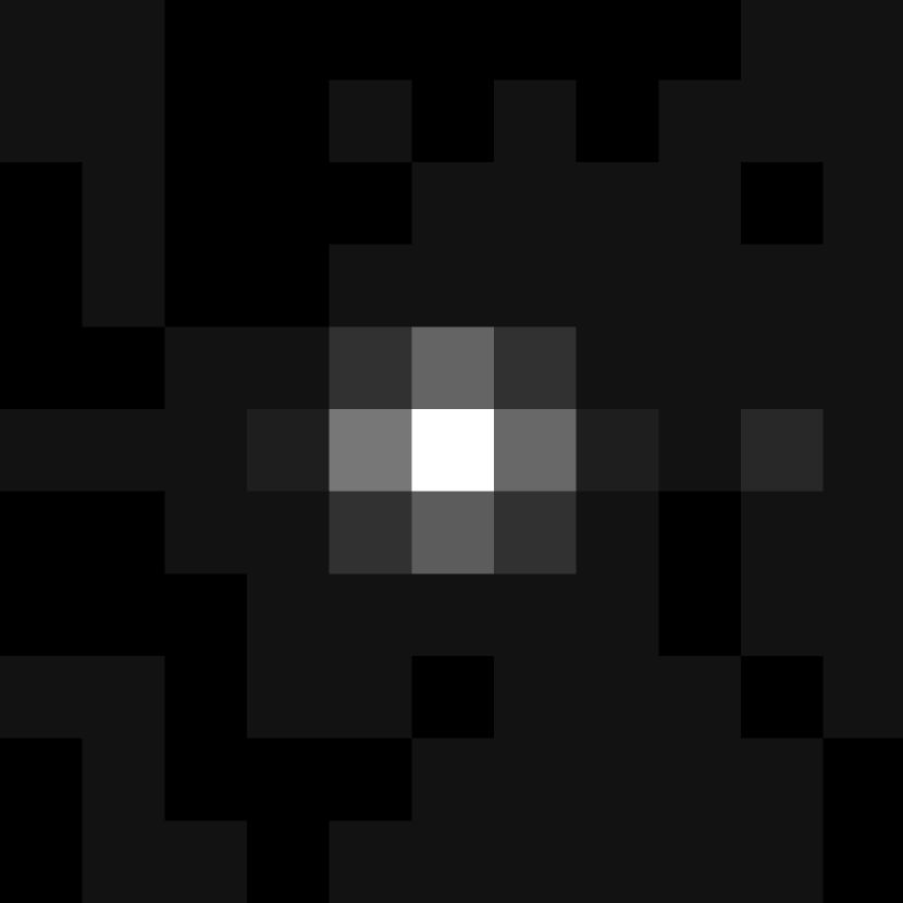
Figure 2: Stacking a large number, $\sim$36, of proton hits from the Si:As data set reveals cross-talk both in the multiplexer and in the detector array. This signal from the cosmic ray spread to its neighbors. One well-understood mechanism for this cross-talk is charge diffusion. The hot pixel to the right of the primary hit is induced by multiplexer cross-talk.

The cross-talk effect was studied and quantified in the InSb data set for a different study (Rauscher et al., 2000). To measure this effect, Rauscher et al. stacked a large number, $\sim$100, of proton hits and the pixels surrounding them. We define the term “edge-neighbors of a pixel” to refer to the four pixels which share an edge with the pixel in question; the “corner-neighbors of a pixel” are those which have a common corner but no common edge with the pixel in question. In the InSb data set, the edge-neighbors of a pixel impacted by a particle hit exhibited a cross-talk-induced signal of about 1.7% of the signal in the central, impacted pixel. The corner-neighbors also showed a cross-talk-induced signal, about an order of magnitude less than the edge-neighbors. Figure 1 shows that multiplexer-induced cross-talk is present in this data set as well, at about the same magnitude as the corner-neighbors. The corner-neighbors and the multiplexer-induced cross-talk are faint with respect to the read noise, typically at or below $3\sigma_{r}$, and thus will be indistinguishable from random noise. This approach was duplicated for the Si:As data set with a set of $\sim$36 proton hits. In the Si:As data set, Figure 2, the magnitude of the cross-talk in the edge-neighbors was about 3.0% of the signal in the impacted pixel, while the corner-neighbors were impacted by about an order of magnitude less than the edge-neighbors. There are also signs of multiplexer-induced cross-talk, also on par with the corner-neighbors. Again, both the corner-neighbor and multiplexer-induced cross-talk are below $3\sigma_{r}$ and should be indistinguishable from random noise.

The net effect of this cross-talk is that most particle events will affect a clump of pixels in a cross or an extended cross in the case of a particle which passes through multiple pixels. In the case of “glancing” cosmic rays, which inject relatively small signals, the signal induced by cross-talk in some or all of the edge-neighbors could fade into the noise, in which case a smaller clump or only one pixel might be affected measurably. One way to increase the ability of the cosmic ray detection algorithm is to add an “impugn neighbors” step, by which we mean either lowering the threshold for finding glitches, or rejecting outright, pixels which neighbor a glitch when one is found. Such a step will add very little to the running time, as the Up-the-Ramp software is already dominated by input (Fixsen et al., 2000). However, we are concerned that adding such a step might cause the cosmic ray identification algorithm to discard excessive amounts of valid data, to the detriment of the overall data quality. Rather than modify the Fixsen et al. algorithm, we apply the algorithm as originally presented to determine the level of its success without adding an “impugn neighbors” step.

The result of a cosmic ray event is the loss of one interval during the Up-the-Ramp observation (potentially plus a few extra intervals if the detector shows persistent effects) for a group of pixels clumped in a (sometimes incomplete) cross-shaped pattern. This loss degrades the quality of the data-fitting routine; on average, the signal-to-noise ratio for a cosmic-ray pixel is reduced by 1/$\sqrt{2}$ for low-signal cases, up to $\sqrt{(N-1)/N}$ for high-signal cases with $N$ samples. Of course, this reduction in signal-to-noise will often be preferable to the alternative, which is total loss. Furthermore, as Fixsen, et al. point out, on-the-fly cosmic ray rejection enables longer integration times, which provides a straightforward way to increase the signal-to-noise to compensate for such loss.

4 InSb Data Set

The InSb data are from a $256\times 256$-pixel InSb (Indium Antimonide) detector array which researchers at the University of Rochester subjected to proton flux at the Harvard Cyclotron.

Each 172-millisecond integration was recorded as one Fowler pair (Fowler & Gatley, 1990), followed by a reset of the detector. As a result, each raw sample of the detector represents an independent 172 ms integration. We use a set of 99 such images. So we can apply the Up-the-Ramp algorithm to this data set, we co-add the independent samples to create an Up-the-Ramp sequence (i.e. The Up-the-Ramp samples are generated from the Raw samples via $U_{0}~{}=~{}R_{0}$, $U_{i}~{}=~{}U_{i-1}~{}+~{}R_{i}$). The set $\{U_{0...98}\}$ approximates a uniformly-sampled data set; for example, the covariance of the samples does not match the form of the covariance assumed in the data processing algorithm (Fixsen, et al., 2000). Since this is an approximation to a Up-the-Ramp sequence, we are making use of less-than-ideal data to conduct this test. However, the differences should be slight and should not affect the overall validity of the results of this test.

The array was irradiated using a 70 MeV beam; the dewar walls attenuated the energy to 20 MeV. The Rochester team conducted these tests with the proton beam emitting $6.5~{}\times~{}10^{4}$ protons cm^-2 s^-1. From the array pixel size of $30\mu{\rm m}~{}\times~{}30\mu{\rm m}$ pixels and the fact that there are $256~{}\times~{}256$ pixels in the detector, we find that the array is impacted by approximately $3.8\times 10^{4}$ protons sec^-1. This is approximately equal to the ion flux which would be expected in deep space at the height of a major solar event, between 3 and 4 orders of magnitude greater than the “typical” cosmic ray flux in deep space, and so represents a severe test of the cosmic ray detection algorithm. (Barth & Isaacs, 1999; Tribble 1995).

The path through the detector array of a cosmic ray from an isotropic distribution is effectively random. However, for the InSb radiation test, the proton beam had a predetermined angle of incidence, 23 degrees from the plane of the detector. Coupled with the InSb pixel dimensions of $30\mu{\rm m}~{}\times~{}30\mu{\rm m}~{}\times~{}8\mu{\rm m}$, we calculate that the projection of the typical proton’s path onto the plane of the detector array is about 19$\mu{\rm m}$ long. If we project this path length onto random locations on the plane of the detector, we find that about half of the protons will pass through 1 pixel and about half will pass through 2 pixels. For this computation, we ignore the effects of scattering and secondary particles.

When a proton physically passes through 1 pixel, cross-talk effects will cause a total of 5 pixels to be affected at the $3\sigma$ level or higher. When a proton passes through 2 pixels, 8 total pixels are affected at $3\sigma$ or higher. If we assume a 50-50 split between these two cases for the InSb data set, an average of 6.5 pixels are affected per proton. Since we expect the InSb detector array will encounter $3.8\times 10^{4}$ protons sec^-1, we find that about 13.8% of the detector array is affected by radiation for each 172 ms second sample. This type of analysis presents difficulties in performing formal uncertainty analysis, but we estimate that these numbers are good to $\pm 25$%.

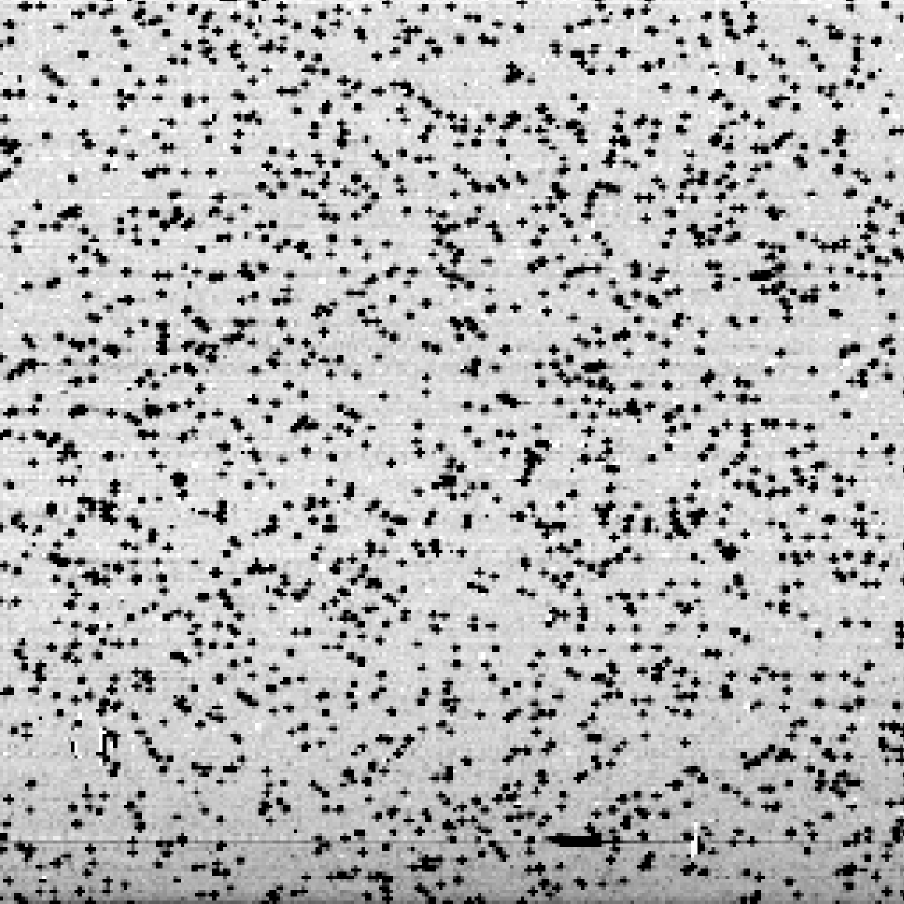
Figure 3: An Up-the-Ramp sample from the InSb data sequence. This is a raw sample ($R_{74}$ in the notation used in Section 4), chosen at random from the observation sequence. Dark pixels in this figure correspond to high-signal regions, light pixels correspond to low-signal regions. Most of the high-signal regions of the detector are due to proton impacts (compare to Figure 4 to see the detector “hotspots”). Since this is the raw difference image, the number of particle hits on the detector is the amount that accumulate in 172 milliseconds.

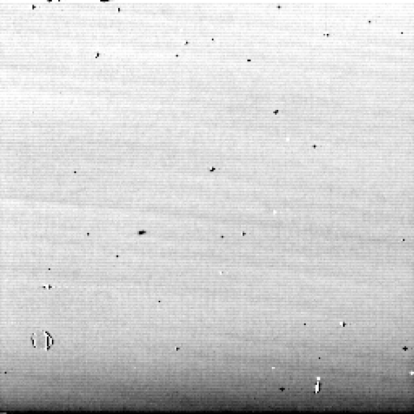
Figure 4: The median image generated from the raw InSb samples. This image was generated for comparison purposes: each pixel is the median value at that pixel across the 99 samples which constitute the raw data set. Most of the high-signal regions are due to “hot spots” on the detector. Also, note the readout glow across the bottom of the detector and the “tree ring” structure across the image.

A sample image from the raw InSb data set appears in Figure 3. This is a raw image, randomly chosen from the original sequence ($R_{74}$ in the notation used earlier), and the number of cosmic rays on this image is that of a single 172 millisecond interval. The images are mostly dark frames. To create a “pseudo-real sky” image for comparison purposes, we create a median image, Figure 4, in which each pixel is the median value of the raw samples for that pixel. We then scale to the full integration time by multiplying the median values by 99, the number of samples in the observation sequence. The result compares favorably with an illuminated flat field frame. The observed “tree ring” structure, representing doping density variations in the InSb, appears in illuminated frames but not in dark current frames. Thus, either there is a small light leak, or the filter wheel has been warmed by proton irradiation, illuminating the array, albeit to a very low level. Similarly, there is a readout “glow”; this effect is present over the entire image but is most pronounced in the first few rows sampled (corresponding to the bottom of the frame).

5 Si:As Data Set

The Si:As data are from a $40\times 40$-pixel region of a $256\times 256$-pixel Si:As (Silicon doped with Arsenic) IBC detector which was subjected to proton flux at the University of California–Davis cyclotron.

The Si:As data set is a series of 52-millisecond integrations, each recorded as a 1 Fowler-pair observation (Fowler & Gatley, 1990), followed by a reset of the detector. A $40\times 40$-pixel subregion of the detector was used; the photo-conducting region of each pixel was approximately $30\mu{\rm m}~{}\times~{}30\mu{\rm m}~{}\times~{}30\mu{\rm m}$. As in the InSb case, the data are dark frames.

We generate an approximate Up-the-Ramp sequence by co-adding 36 independent samples using the same procedure described in Section 4. The caveats regarding the use of this approximation which were discussed in Section 4 apply to the Si:As data as well. These differences still should not affect the overall validity of the results of this test.

The array was irradiated with a 67 MeV proton beam operating in an uncalibrated mode (i.e. the proton flux is not independently known). The proton beam passed through only a thin plastic window on its way to the detector—there was no dewar wall in the proton beam path, as there was in the InSb data set. As a result, the protons should not be scattered or attenuated appreciably.

As the proton flux was not directly measured, the only source of information with regard to the number of events expected on the detector is the data set itself. We estimate the number of events by examining a sequence of 36 raw (difference) samples and counting the number of outliers from the background dark value as a function of the outlier threshold; we expect the read noise to be a Gaussian distribution and thus the number of outliers due to read noise should fall off in a Gaussian pattern as we increase the threshold. Outliers caused by protons, which should be large with respect to the dark value, will not fall off at low multiples of $\sigma$. In the sample we tested, the number of outliers flattened out in the interval 4$\sigma$-to-5$\sigma$. If we use these values as the lower and upper limits for the threshold, we find that between 3.0% ($4\sigma$) and 2.4% ($5\sigma$) of the pixels should be identified as particle hits or neighbors impacted by cross-talk for each interval. For a 36-frame sequence of $40\times 40$-pixel images, we expect to find around $1500~{}\pm~{}200$ pixels impacted by cosmic rays during the observation. This figure includes pixels impacted both by cosmic rays and by cross-talk (see Section 3). Since the proton beam was oriented normal to the plane of the detector, most of the protons would physically pass through one pixel; based on the cross-talk model, we expect that $\sim$20% of the glitches are cosmic-ray hits, the rest being caused by cross-talk. We find that the cosmic ray flux is approximately $1.1\times 10^{4}$ protons s^-1 cm^-2. This flux is about a factor of 6 lower than that used in the InSb test.

The signal in the Si:As images is heavily quantized (i.e. the histogram of the data values is fairly sparse). The statistical tests used to identify the cosmic ray glitches and the line-fitting algorithm from Fixsen, et al. will perform best when the data are continuous or the level of quantization is small relative to the size of the data. Although we do not expect this to be a major problem, the uncertainty in the results from the line-fitting routine may be larger than it would otherwise be.

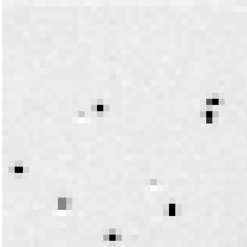
Figure 5: An Up-the-Ramp sample from the Si:As data sequence. This is a raw sample ($R_{27}$ in the notation used in Section 4), chosen at random from the observation sequence. Dark pixels in this figure correspond to high-signal regions, light pixels correspond to low-signal regions. Most of the high-signal regions of the detector are due to proton impacts (compare to Figure 6). Since this is the raw difference image, the number of particle hits on the detector is the amount that accumulate in 52 milliseconds.

A sample image from the raw Si:As data set appears in Figure 5. This is a raw image, randomly chosen from the original sequence ($R_{27}$ in the notation used in Section 4), and the number of cosmic rays on this image is that of a single interval, 52 milliseconds. To create a “pseudo-real sky” image for comparison purposes, we create a median image, Figure 6, in which each pixel is the median value of the raw samples for that pixel. We then scale to the full integration time by multiplying the median values by 36, the number of samples in the observation.

6 InSb Results & Discussion

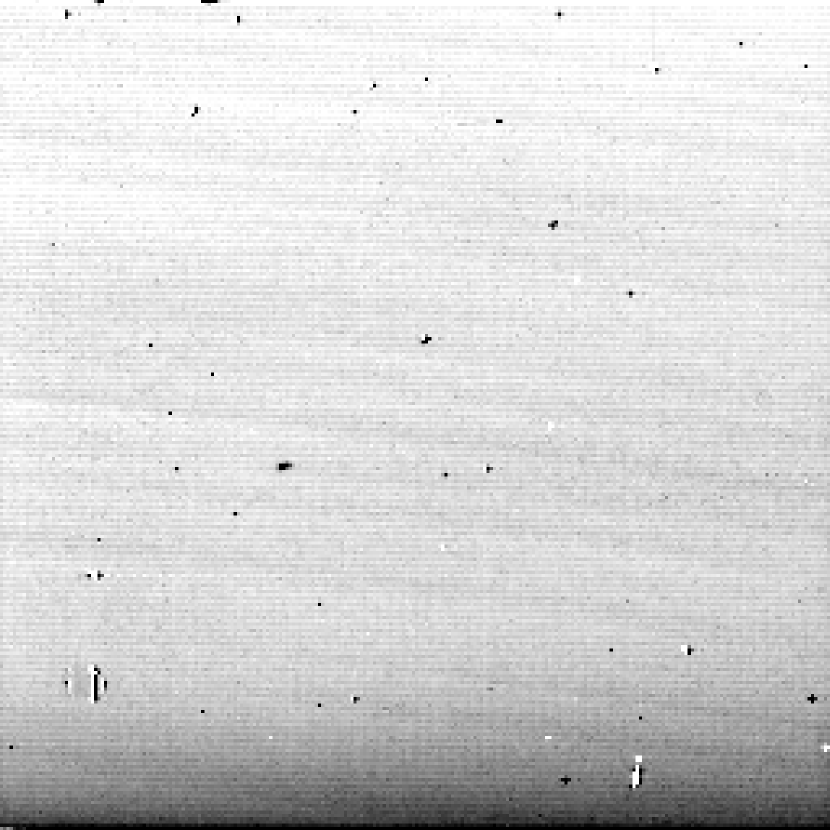
Figure 7: The output data image from processing 99 InSb data samples. Compare with Figure 4—there is a high correspondence between high-signal pixels in this image and those in Figure 4. Note that the glow at the bottom of the detector and the “tree ring” structure are preserved in this output image.

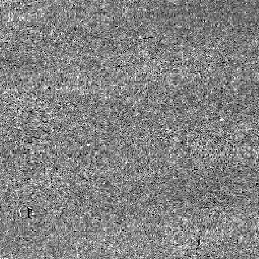
Figure 8: The difference between Figure 7 and Figure 4. In this image, dark pixels correspond to regions where Figure 7 has a higher signal; light pixels correspond to regions where Figure 4 has a higher signal; regions where the two images are equal are grey. The greyscale spread covers $\pm 3\sigma_{r}$.

The output data image from the processing the 99 InSb samples appears in Figure 7. A difference image between this image and the median image appears in Figure 8. Figure 9 shows the pattern of cosmic rays identified in a randomly-chosen sample (the same sample that is shown in Figure 3).

We perform one simple tuning operation with this data set to verify that the cosmic ray threshhold of $4.5\sigma$ used by Fixsen, et al. was appropriate for this data set. We divide the 99-image sequence of InSb samples into two 49-image sequences (discarding one), and generate two Up-the-Ramp sequences. The two sequences are then processed using a series of cosmic ray rejection threshholds, generating one pair of output images for each threshhold value. We measure the uncertainty of the threshhold value as the RMS difference between the two images of each pair for that value. We examine the threshholds to be in the range of $1-7\sigma$ equally spaced at intervals of $0.5$ (i.e. $[1,1.5,2,2.5,...,7]\sigma$). The initial pass shows a minimum between $4\sigma$ and $5\sigma$, so we repeat the test between these two values at intervals of $0.1$. The results are shown in Figure 10; the minimum appears at $4.5\sigma$. Because there are insufficient samples to repeat this test reliably with the Si:As data set, we adopt $4.5\sigma$ as the threshhold value for that data set as well. We also find median image for the two subimage sequences, and compute the RMS difference for the two median images. The RMS difference at $4.5\sigma$ is 3.24, compared with the value of 2.33 for the median case; however, if we discard the pixels for which contain a surviving cosmic ray in either image of each set (27 pixels in the Up-the-Ramp case, 49 pixels in the median case), the Up-the-Ramp RMS difference drops to 1.34, whereas the RMS for the median images is 1.37.

As discussed in Section 4, we find that 13.8% of the detector should be affected by a proton or by cross-talk for each sample; the total number of pixels affected by protons plus those affected by cross-talk comes to 895,000 for the entire sequence ($\pm 224,000$, using our ballpark estimate of 25% for the uncertainty in this number). The cosmic ray rejection algorithm, with the minimal tuning, identifies and rejects 1,063,000 bad samples from this observation sequence. This number lies within the uncertainty range for the number of expected bad samples. We must be cautious against reading too much into this result, but it is safe to say that the number of cosmic rays identified is in the right ballpark. The overall performance can be improved by tuning the parameters of the algorithm, which will require repeated and detailed radiation tests with the detector.

An examination of Figure 9 shows that most of the cosmic ray detections are clumped in cross-hatch patterns, matching the current-leak pattern described in Section 3. Thus, the cosmic-ray identification algorithm catches many of the neighboring pixels affected by cross-talk without having to add an “impugn neighbors” step, as described in Section 3. When the full energy spectrum of cosmic rays in deep space is considered, the amount of charge injected, and the resulting signal, will often be smaller than that induced by a cyclotron proton. The fact that the cosmic ray identification algorithm catches the neighbor-leak events shows that it is capable of identifying the full spectrum (i.e. bright, faint and in-between) of cosmic rays that we expect to encounter in a deep space environment (contrasted with the limited particle energy spectrum generated by the cyclotron). As this is a dark frame, faint bad pixels stand out from their neighbors; the current cosmic ray identification software might not work as well in brighter regions of the image, where increased Poisson noise will affect the statistical test used to identify cosmic rays. Brighter images and fainter cosmic rays will combine to mask the “neighbor-leak” events—tuning the algorithm to the specific detector would minimize the impact of these effects, but a step to “impugn neighbors” might still be required during astronomical observations.

The frames in this study are dark frames. As was discussed in Section 4, there appears to be a small light leak or thermal glow which is faintly illuminating the array as a whole. There is also an apparent “glow” effect, which is most prominent in the first few rows sampled (the bottom of the image in the orientation shown in Figure 4 and Figure 7). The only other non-random contributions to the flux should be the dark current, “hot” pixels and other detector artifacts. By taking the image generated from performing the median operation on the raw data set, Figure 4, and scaling up from 1 sample to 99 by multiplication, the dark value is computed to be $4880~{}\pm~{}41$ data units (1.8 electrons per data unit). The dark value on the processed image is computed to be $4881~{}\pm~{}40$ data units—the median and processed median dark values agree very strongly, well within the margin for error. In addition, note that the readout “glow” at the bottom of the image as well as the faint “tree ring” structure over much of the detector, both of which appear in Figure 4, are preserved in Figure 7 (both of those effects can be mistaken for errors in printing or reproduction, but they are genuine).

Overall, the processed image and the median image agree very well at most individual pixels to within the uncertainty of the dark level established in the previous paragraph. 99.5% of all pixels agree within this tolerance; most of the remainder are surviving cosmic rays. This result, combined with the estimated number of cosmic ray events derived earlier, suggests that the cosmic ray algorithm successfully identified and removed over 99.96% of the proton events on the detector.

We examine in detail the pixels in which the processed image and the median/comparison image disagree by at least $3\sigma$. A total of 88 pixels fit into this category; 44 of them occur in places where both of the images are high-signal (detector hotspots), and thus where we expect that higher Poisson noise, non-linear response and other effects increase the normally-expected noise. Of the remaining 44 instances, 35 are cases where the processed image is brighter than the median image; these are cosmic rays which were missed by the cosmic ray detection algorithm. The remaining 9 instances, where the processed image is darker, are all cases where more than half of the samples were affected by cosmic rays, so the median of the sample is a cosmic ray sample—these 9 pixels contain cosmic rays which were caught by the algorithm in Fixsen, et al., but which the median operation missed.

7 Si:As Results & Discussion

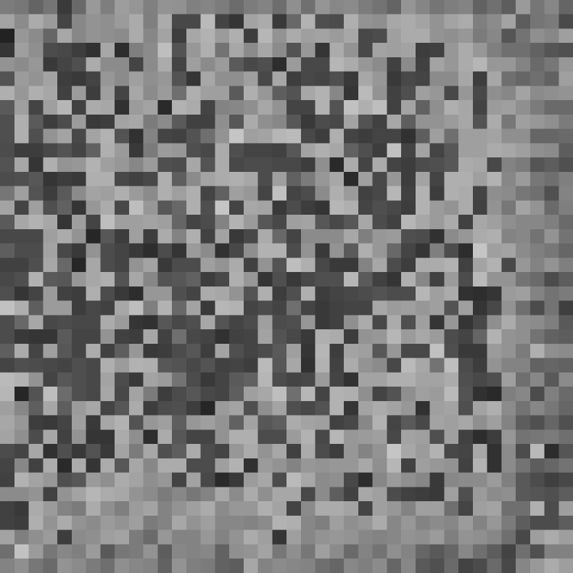
Figure 12: The difference between Figure 11 and Figure 6. In this image, light pixels correspond to regions where Figure 11 has a higher signal; dark pixels correspond to regions where Figure 6 has a higher signal; regions where the two images are equal are grey. Overall, there is no spatial difference or trend. The quality of this image is limited by the severe quantization of Figure 6.

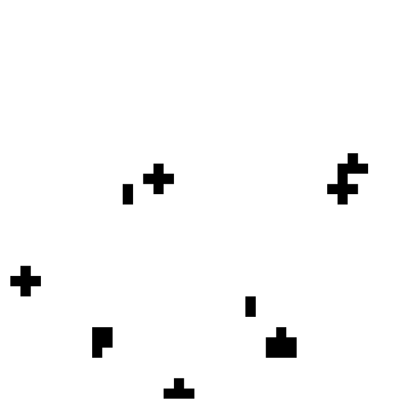
Figure 13: The cosmic ray mask for the sample shown in Figure 5. The dark pixels show the places where cosmic rays were identified and removed from this sample. Note that the pattern of glitches is similar to the cross-hatching pattern described in Section 3.

The output data image from the processing the 36 Si:As samples appears in Figure 11. A difference image between this image and the median image appears in Figure 12. Figure 13 shows the pattern of cosmic rays identified in a randomly-chosen sample (the same sample that is shown in Figure 5).

As discussed in Section 5, we expect to find $1500~{}\pm~{}200$ pixels affected by a proton or cross-talk during the full 36-sample observation. The cosmic ray rejection algorithm, with only the minimal tuning described in Section 1, identifies and rejects 1230 bad samples during the observation sequence. This number lies outside of the uncertainty range for the number of expected bad samples, but by a small margin. Again, the result is promising.

An examination of Figure 13 shows that most of the cosmic ray detections are clumped in cross-hatch patterns, again matching the current-leak pattern described in Section 3. As was the case with the InSb case, this shows that the cosmic-ray identification algorithm catches the neighbors affected by cross-talk without requiring any extra steps.

The Si:As images are dark frames; the only non-random signals are from dark current and detector artifacts. By taking the median image (Figure 6) and scaling from 1 sample to 36 by multiplication, the dark value is found to be $375~{}\pm~{}9$ data units, compared to the processed image’s dark value of $348~{}\pm~{}6$ data units—the dark values for these images agree to within 3$\sigma$. If we compare Figure 6 and Figure 11, we see that the signal along the bottom and right-hand side of the detector are preserved in the output image, although heavy quantization limits the amount of observable structure in the median image.

Overall, the processed and median images disagree by more than 3 times the uncertainty of the processed image at 5 pixels. In all 5 cases, the processed image has a lower signal than the median image by just over $3\sigma$ (3.01–3.12$\sigma$). These deviations appear to be caused by error in the data fitting routine due to the heavy quantization of the input data. As the proton hits will bias the median image towards higher signals, we recomputed the median image, discarding reads which differ from the mean by more than $3\sigma$. Removal of this bias reduces the number of different pixels to 3. As the large quantization adds noise to the median which will be less pronounced in the processed data, the median may be a less accurate measure of the “real sky” than the output image. There do not appear to be any missed cosmic rays in the output image.

8 Conclusion

The Up-the-Ramp sampling and on-the-fly cosmic ray rejection algorithm performs excellently on the radiation test data from the InSb and Si:As detectors, particularly when we consider that the data were not originally Up-the-Ramp samples (but co-added intervals), the algorithm parameters were only minimally tuned to the detector, the data were not linearized before processing and we ignored any possibility of persistent radiation effects, which is particularly important since the particle rates were extremely high. Detailed tuning of the algorithm with the experiment detector will improve these results. The cosmic ray algorithm did not introduce any 2-D structure into the image, and preserved the structure which was there. Finally, the small number of pixels for which the median and processed images which differed significantly shows that the Up-the-Ramp sampling can and does preserve the photometric quality of the data.

We have attempted to answer some common concerns about the use of Up-the-Ramp sampling strategies. We have shown that the algorithm performs well without precise tuning to the detector characteristics, as we have obtained good performance without such tuning. Another concern is that the cosmic-ray/detector interaction model assumed in the design of the algorithm is too simplistic; however, the results here show good performance without requiring additional complicating features. In short, we haven’t found any “show-stoppers” that would lead to the conclusion that the algorithm requires excessive computing or human interaction to provide useful scientific data.

These results are limited to the detector technologies being studied here. A key future direction for this study is to apply the techniques discussed here to additional detector technologies (such as HgCdTe technology, used in the NICMOS instrument on HST). This is particularly true in the context of detector characterization studies for observatories and instruments being designed currently or in the near future, which is how this study started. However, the fact that we obtain very similar results with the two technologies suggests that the cosmic ray mitigation approach studied here could be applied to many instruments and detectors.

Appendix A Signal-to-Noise

We selected Up-the-Ramp sampling for study because it provides better signal-to-noise in what is probably the most difficult-to-measure regime, the read-noise limit. In the absence of cosmic rays, Up-the-Ramp sampling provides modestly ($\sim 6\%$) higher signal-to-noise than does Fowler Sampling (Garnett & Forrest, 1993). The fact that an Up-the-Ramp sequence can be screened for cosmic rays and other glitches improves this result. Furthermore, on-the-fly cosmic ray rejection allows longer integration times which also improves the signal-to-noise in the faint limit.

Fowler sampling reduces the effect of read noise to $\sigma^{\prime}_{r}~{}=~{}\sigma_{r}\sqrt{\frac{4}{N}}$ (for an observation sequence consisting of $N$ samples, $N/2$ Fowler-pairs). However, when a pixel is impacted by a cosmic ray during an observation, the cosmic ray essentially injects infinite variance and reduces the signal to noise to zero at that location. If we start with the Fowler sampling signal-to-noise function in the read-noise limit, from Garnett & Forrest (1993, Eqn. 6),

$$SN_{F}=\frac{FT}{\sqrt{2}\sigma_{r}}\sqrt{\frac{\eta T}{2\cdot\delta t}}\left(1-\frac{\eta}{2}\right)=\frac{FT}{\sqrt{V_{0}}}$$ (A1)

where $F$ is the flux of the target, $T$ is the observation time, $\sigma_{r}$ is the read noise, $\eta$ is the Fowler duty cycle and $\delta t$ is the time between sample intervals (determined by engineering or scientific constraints on the system). We note this formula breaks down for relatively small numbers of samples (i.e. $\delta t$ large with respect to $T$). $FT$ is the signal, so the remaining terms are the noise, which is the square-root of the variance, $V_{0}$. If we consider two cases, “no-cosmic-ray” and “hit-by-cosmic-ray” and combine the variances according to

$$V_{comb}=\frac{V_{0}P_{0}W_{0}^{2}+V_{1}P_{1}W_{1}^{2}}{(W_{0}P_{0}+W_{1}P_{1})^{2}}$$ (A2)

we can rewrite Equation A1 as

$$SN_{FC}=\frac{FT}{\sqrt{V_{comb}}}=\frac{FT(W_{0}P_{0}+W_{1}P_{1})}{\sqrt{V_{0}P_{0}W_{0}^{2}+V_{1}P_{1}W_{1}^{2}}}$$ (A3)

As the weight is the inverse of the variance ($W_{i}=1/V_{i}$), Equation A3 can be rewritten as

$$SN_{FC}=\frac{FT(\frac{P_{0}}{V_{0}}+\frac{P_{1}}{V_{1}})}{\sqrt{P_{0}/V_{0}+P_{1}/V_{1}}}=FT\sqrt{\frac{P_{0}}{V_{0}}+\frac{P_{1}}{V_{1}}}$$ (A4)

$V_{0}$ is the variance in the no-cosmic-ray case, taken from Equation A1 and $P_{0}$ is the probability of a pixel surviving without a cosmic ray hit. For simplicity, we define $1-P$ to be the probability of a pixel being hit by a cosmic ray per time unit $\delta t$, so $P$ is the probability of “survival” and $P_{0}=P^{T/\delta t}$. As a cosmic ray hits injects infinite uncertainty, the variance in the cosmic ray case $V_{1}=\infty$. Plugging in to Equation A4, we get the signal-to-noise for Fowler sampling in the read-noise limited with cosmic rays, Equation A5:

$$SN_{FC}=FT\sqrt{\frac{P_{0}}{V_{0}}+0}=\frac{FT}{\sqrt{2}\sigma_{r}}\sqrt{\frac{\eta T}{2\cdot\delta t}}\left(1-\frac{\eta}{2}\right)P^{T/(2\cdot\delta t)}$$ (A5)

For a given integration time $T$ and minimum read time $\delta t$, the maximum $SN_{FC}$ occurs with duty cycle $\eta=2/3$. If we plug this back into Equation A5, we get

$$SN_{F}=\frac{2}{3}\frac{FT}{\sqrt{2}\sigma_{r}}\sqrt{\frac{T}{3\delta t}}P^{T/(2\cdot\delta t)}$$ (A6)

From here, it is possible to find the value of $T$ which gives the best signal-to-noise for a single observation; it occurs at $T~{}=~{}-3\cdot\delta t/\ln(P)$. If, however, we consider the observation as a series of $M$ equal observations with a specific total observation time, $T_{obs}$, the signal-to-noise for the series is

$$SN_{FC}^{{}^{\prime}}=\frac{FT\sqrt{M}}{3\sigma_{r}}\sqrt{\frac{2T}{3\delta t}}P^{T/(2\cdot\delta t)}=\frac{FT\sqrt{T_{obs}}}{3\sigma_{r}\sqrt{T}}\sqrt{\frac{2T}{3\delta t}}P^{T/2\cdot\delta t}$$ (A7)

If we hold $T_{obs}$ constant and find the optimum $T$, we find that it is $T~{}=~{}-2\cdot\delta t/\ln(P)$. In either case, it is important to note that, in there is an optimal value for $T$, and extending the observation beyond that time will ruin the data.

It is worth noting that the result assumes that all cosmic ray events can be identified a posteriori. This is not necessarily the case, particularly when it is considered that, in the one-image case, the fraction of pixels surviving without a cosmic ray impact is $P^{-3/\ln(P)}=e^{-3}\approx 0.05$; for the multi-image case, the fraction of survivors is $P^{-2/\ln(P)}=e^{-2}\approx 0.14$. In both cases, the number of “good” pixels is so low that separating them from the impacted pixels will not be a trivial task. For example, the median operation would not be able to identify a good samples, as more than half of the samples would be impacted by cosmic rays. In practice, the detector will often saturate before this limit is reached, but this shorter integration time means that less-than-optimal signal-to-noise will be obtained.

Up-the-Ramp sampling reduces the effect of read noise to $\sigma^{\prime}_{r}~{}=~{}\sigma_{r}\sqrt{\frac{12}{N}}$, for N uniformly-spaced samples with equal weighting (which is the optimal weighting for the read-noise limited case). When a pixel is impacted by a cosmic ray, the Up-the-Ramp algorithm preserves the “good” data for that pixel. The exact quality of the preserved data depends on the number of cosmic ray hits and their timing within the observation. For example, a cosmic ray hit which just trims off the last sample in the sequence has minimal impact compared to a cosmic ray hit that occurs in the middle of the observation sequence. The variance of a Uniformly-sampled sequence with $N_{i}$ samples is proportional to $1/N_{i}(N_{i}+1)(N_{i}-1)$. If an Up-the-Ramp sequence is broken into $i$ chunks by a cosmic ray, the variance becomes

$$V_{i}=V_{U}\frac{N(N+1)(N-1)}{\sum_{j=0}^{i}(N_{j})(N_{j}+1)(N_{j}-1)}$$ (A8)

When there are zero cosmic ray events, of course, $V_{0}=V_{U}$. If there is one cosmic ray event during the sequence, the variance becomes

$$V_{1}~{}=~{}V_{U}~{}\frac{N(N+1)(N-1)}{N_{i}(N_{i}+1)(N_{i}-1)+(N-N_{i})(N-N_{i}+1)(N-N_{i}-1)}$$ (A9)

If we assume (as is reasonable) that the cosmic ray events are randomly distributed over time and find the expectation value for all values of $0...N_{i}...N$, we find that the typical $V_{1}~{}\approx~{}V_{U}*2$ (plus a small term in $N^{-1}$, which we will ignore for simplicity). If we perform a similar computation for two cosmic ray events, we find that $V_{2}~{}\approx~{}V_{U}*10/3$ (again, plus lower-order terms which we ignore). In general, we find that it is possible to find a valid result with a finite (although not necessarily pretty) variance for any sequence broken up by cosmic ray events provided we have at least 2 consecutive “good” samples (for all practical purposes, we can ignore the situation where this is not the case). To simplify the following, we will simplify by considering only 3 cases: The no-cosmic-ray case $V_{0}=V_{U}$, the one-cosmic-ray case $V_{1}=2*V_{U}$ and all multiple-cosmic-ray cases combined as one, $V_{2+}=V_{U}/\epsilon^{2}$, where $\epsilon^{2}$ is a small but non-zero number, roughly 0.3.

The Up-the-Ramp signal-to-noise function for the read-noise limited case (Garnett & Forrest, 1993, Eqn. 20) is

$$SN_{U}=\frac{FT}{\sqrt{2}\sigma_{r}}\sqrt{\frac{N^{2}-1}{6N}}=\frac{FT}{\sqrt{V_{U}}}$$ (A10)

We combine the variances in the 3 possible cases with the three-case equivalent to Equation A2, and thus arrive at

$$SN_{UC}=FT\left(\frac{P_{0}}{V_{0}}+\frac{P_{1}}{V_{1}}+\frac{P_{2+}}{V_{2+}}\right)^{1/2}=\frac{FT}{\sqrt{V_{U}}}\left(P_{0}+\frac{P_{1}}{2}+\epsilon P_{2+}\right)^{1/2}$$ (A11)

where $P_{i}$ is the probability of a pixel being impacted by $i$ cosmic rays during the integration. We note, as did Garnett & Forrest, that there would be no reason to limit the number of samples to anything less than the maximum possible number, so we can set $N~{}=~{}T/\delta t$. Using the definition of $P$ described earlier, $P_{0}~{}=~{}P^{T/\delta t}$, $P_{1}~{}=~{}(T/\delta t)\cdot(1-P)P^{T/\delta t-1}$ and $P_{2+}~{}=~{}1-(P_{0}+P_{1})$. Putting these values back into Equation A11, we get:

$$SN_{UC}=\frac{FT}{\sqrt{2}\sigma_{r}}\sqrt{\frac{T^{2}-\delta t^{2}}{6T\delta t}}\left[(1-\epsilon)P^{T/\delta t}+(1-\epsilon)\frac{T}{\delta t}(1-P)P^{T/\delta t-1}+\epsilon\right]^{1/2}$$ (A12)

If we seek the maximum value of $SN_{UC}$ with respect to $T$, we find that $\partial(SN_{UC})/\partial T~{}>~{}0$, provided $T~{}\geq~{}\delta t$ (otherwise we’d have an integration shorter than 1 sample time, which would be useless), $P\neq 0$ and $0<\epsilon<1$ (both of which are true by construction). This result applies equally whether we are considering one independent integration or a series of observations to be combined further downstream. As the derivative is strictly positive, the signal-to-noise continues to increase with as sample time increases, although as $T~{}\rightarrow~{}\infty$, the gain in signal-to-noise asymptotically approaches zero. So, extending the observing time while using Up-the-Ramp sampling with cosmic ray rejection does not damage the data (although we might be spending time with little or no gain). As noted earlier for the Fowler-sampling case, there is an optimal observing time, beyond which further observation reduces the overall signal-to-noise.

Figure 1: Stacking a large number, $\sim$100, of pixel proton hits from the InSb data set reveals cross-talk both in the multiplexer and in the detector array. In time, the hot pixel 4 pixels to the right of the primary hit was the next pixel read out—this hot pixel is referred to as the “MUX bleed.” Moreover, the hit is not confined to one pixel. Rather, it spreads to its neighbors. One well understood mechanism governing this cross-talk is charge diffusion.

Figure 6: The median image generated from the raw SiAs samples. This image was generated for comparison purposes: each pixel is the median value at that pixel across the 36 samples which constitute the raw data set. The region sampled for this test is $40\times 40$ pixels; the pixellation in this image and the other Si:As images is caused by scaling the image up to the size shown here. The data in the Si:As set are severely quantized, which reduces the quality of this image.

Figure 9: The cosmic ray mask for the sample shown in Figure 3. The dark pixels show the places where cosmic rays were identified and removed from this sample. Note that the cross-hatching pattern matches the cross-talk pattern described in Section 3.

Figure 10: The RMS differences for the InSb data set plotted as a function of cosmic ray rejection threshold. The minimum occurs around $4.5\sigma$. The value of $4.5$ is used for the cosmic ray rejection threshold for all results discussed in this paper.

Figure 11: The output data image from processing 36 Si:As data samples. Compare with Figure 6.

References

- (1) Barth, J. & Isaacs, J., 1999, “The Radiation Environment for the Next Generation Space Telescope.” http://ngst.gsfc.nasa.gov/cgi-bin/pubdownload?Id=570
- (2) Fanson, J. L., Fazio, G. G., Houck, J. R., Kelly, T., Rieke, G. H., Tenerelli, D. J. & Whitten, M., 1998, Proc. SPIE, 3356, 478.
- (3) Fixsen, D. J., Offenberg, J. D., Hanisch, R. J., Mather, J. C., Nieto-Santisteban, M. A., Sengupta, R. & Stockman, H. S., 2000, PASP, 112, 1350-9.
- (4) Fowler, A. M., & Gatley, I., 1990, ApJ, 353, L33-4.
- (5) Garnett, J. D. & Forrest, W. J., 1993, Proc. SPIE, 1946, 395.
- (6) Holloway, H., 1986, J. Appl. Phys., 60, 1091
- (7) Offenberg, J.D., Sengupta, R., Fixsen, D.J., Stockman, H.S., Nieto-Santisteban, M.A., Stallcup, S., Hanisch, R.J., & Mather, J.C. 1999, in Astronomical Data Analysis Software and Systems VIII D.M. Mehringer, R.L. Plante, & D.A. Roberts, Eds. Astron. Soc. Pacific Conference Series, 172, 141.
- (8) Rauscher, Bernard J., Isaacs, John, & Long, Knox, 2000, “Cosmic Ray Management on NGST 1: The Effect of Cosmic Rays on Near Infrared Imaging Exposure Times.” http://www.ngst.nasa.gov/cgi-bin/doc?Id=649
- (9) Stockman, H.S., ed., 1997, The Next Generation Space Telescope: Visiting a Time When Galaxies Were Young, Association of Universities for Research in Astronomy, Inc. http://sso.stsci.edu/second_decade/PDF/bg_docs/NGST.pdf
- (10) Stockman, H. S., Fixsen, D., Hanisch, R. J., Mather, J. C., Nieto-Santisteban, M., Offenberg, J. D., Sengupta, R. & Stallcup, S., 1998, The Next Generation Space Telescope: Science Drivers and Technological Challenges, 34th Liege Astrophysics Colloquium, June 1998, p. 121
- (11) Tribble, A. J., 1995, The Space Environment, Princeton Univ. Press, Princeton, NJ.
- (12)