Ultraviolet Galaxy Counts from STIS Observations of the Hubble Deep Fields.

Abstract

We present galaxy counts in the near-ultraviolet (NUV; 2365Å) and far-ultraviolet (FUV; 1595Å) obtained from Space Telescope Imaging Spectrograph (STIS) observations of portions of the Hubble Deep Field North (HDFN), the Hubble Deep Field South (HDFS), and a parallel field near the HDFN. All three fields have deep (AB$>$29) optical imaging, and we determine magnitudes by taking the ultraviolet flux detected within the limiting optical isophote. An analysis of the UV-optical colors of detected objects, combined with a visual inspection of the UV images, indicates that there are no detectable objects in the UV images that are not also detected in the optical. We determine our detection area and completeness as a function of magnitude with a simulated distribution of galaxies based on the HDFN Wide Field Planetary Camera 2 (WFPC2) V+I image. The galaxy counts reach to $NUV_{AB}=29$ and $FUV_{AB}=30$, which is 1 magnitude fainter than the HDFN WFPC2/F300W counts, and 7 magnitudes fainter than balloon-based counts. We integrate our measurements to present the extragalactic background radiation coming from resolved objects. The NUV galaxy counts show a flattening or turnover beginning at about $NUV_{AB}=26.0$, which is not predicted either by no-evolution models based upon a local luminosity function with a steep faint end slope, nor by a semi-analytic model in which starbursts are caused by major mergers. The FUV counts also show a flat slope. We argue that the flat slopes could be caused by a short duty cycle for star formation, additional starbursts triggered by minor mergers, and an extended quiescent phase between starburst episodes.

Accepted for publication in the Astrophysical Journal Letters

1 Introduction

Imaging of random fields at high galactic latitude is a powerful tool for investigating galaxy formation and evolution. Number counts of galaxies, as a function of filter bandpass, have provided the first solid evidence for the evolution of the normal galaxy population (e.g., Tyson 1988; Lilly, Cowie & Gardner 1991). Much work has been done in the optical and near-infrared, and the number counts of galaxies are now well established observationally at bright magnitudes through wide-area surveys done both with electronic detectors (Gardner et al. 1996) and photographic plates (Maddox et al. 1990). At faint magnitudes, the Hubble Deep Field projects have established the galaxy counts in the optical and near-infrared to AB=30 magnitude (Williams et al. 1996; Thompson et al. 1999; Gardner et al. 2000; Ferguson, Dickinson & Williams 2000). The AB magnitude system is defined by $AB=-2.5log(F_{\nu})-48.6$ where $F_{\nu}$ is given in erg cm^-2 s^-1 Hz^-1 (Oke 1971).

Bright galaxy counts in the ultraviolet have been measured from balloon-borne imaging in the 2000Å window by the FOCA experiment (Milliard et al. 1992), with follow-up ground-based optical spectroscopy by Treyer et al. (1998) and Sullivan et al. (2000). With a 40 cm telescope, FOCA surveyed a total area of about 6 square degrees near the North Galactic Pole over the magnitude range $17.75<F(2000)_{AB}<20.75$, measuring a nearly Euclidean slope for the counts. The colors and spectra of their detected galaxies are consistent with an actively star-forming population dominated by Sdm or later types in the redshift range $0<z<0.5$. The data show a larger population of UV-emitting galaxies than had previously been assumed (Armand & Milliard 1994), with a steep faint-end slope for the UV luminosity function.

In this Letter, we present faint galaxy counts in the near- and far-ultraviolet (NUV & FUV) obtained by imaging several fields with the Space Telescope Imaging Spectrograph (STIS; Kimble et al. 1998; Woodgate et al. 1998).

2 Description of the data

We have examined three datasets. The largest field consists of follow-up STIS imaging of part of the Hubble Deep Field North (HDFN-Fol; Williams et al. 1996), and contains 6 fields of view with the FUV and NUV detectors. The second field consists of the primary STIS observations of the Hubble Deep Field South (HDFS-Pri; Gardner et al. 2000). The third field was a parallel field imaged with STIS in the optical and ultraviolet during a deep imaging campaign of the HDFN (hereafter HDFN-Par) done with NICMOS (Thompson et al. 1999). It is located $\sim 8.5\arcmin$ East of the deep field. All observations used the F25QTZ filter, and are dark noise limited in both the FUV and NUV. These data have been used for a measurement of the diffuse FUV background emission (Brown et al. 2000). Details of the field and the FUV exposure times are given in that paper. The NUV exposure times range from 16,865s to 22,616s per field of view.

We used the public reduction of the HDFS-Pri field (Gardner et al. 2000), and reduced the data on the HDFN-Fol and HDFN-Par fields in the same way. All of the exposures are dithered, which results in a variable exposure time across the final images. In addition, the presence of the FUV dark glow (described in detail by Gardner et al. 2000 and Brown et al. 2000) results in noise that varies by a factor of 2 across the field.

All three fields have deep optical imaging, reaching a 3$\sigma$ limiting AB magnitude of $\gtrsim$29. The HDFN-Fol and HDFS-Pri fields are contained within the deep optical fields. The HDFN-Par field was observed with STIS in the 50CCD mode for 34,076 s. The HDFN-Par observations were made during the first NICMOS camera 3 campaign when the focus of the telescope was changed, and are therefore slightly out of focus, and somewhat less sensitive to point sources than they would otherwise be. However, we do not make a distinction between point sources and extended sources in our analysis, and we take source size into account in our determination of the galaxy counts, so this will not affect our results.

2.1 Object detection and photometry

We used the publicly released SExtractor (Bertin & Arnouts 1996) version 2 catalog for the HDFS-Pri field, and followed a similar procedure for object detection and photometry on the other two fields. As SExtractor has problems handling quantized low-signal data, we computed the flux in the UV images within the pixels assigned to each object in the optical, with local background subtraction. See Gardner et al. (2000) for a more detailed discussion of this procedure. We have made the assumption that there are no objects detectable on the UV images that are undetected on the optical images. Visual inspection of the images confirms this assumption. In addition, the photometry are isophotal magnitudes, where the isophote has been determined in the optical.

In Figure 1 we plot the UV-optical colors of the detected galaxies in the HDFN-Fol field. The optical flux is determined from the SExtractor version 2 catalog of the sum of the HDFN F814W and F606W images (hereafter VI). We plot as a solid line the location on this figure where objects with VI_AB=30 would be, and as a dotted line where objects with VI_AB=29 would be. If we take $VI_{AB}$=29 as the completeness limit for the HDFN catalog, then there are only three galaxies detected at the $3\sigma$ limit in our NUV catalog and no galaxies in our FUV catalog that are fainter than this in the optical. The three galaxies are fainter than $NUV_{AB}$=28 in the UV, and the UV-optical color distribution does not show a sharp cut-off at the optical detection limit.

2.2 Measurement of the number counts

There has been considerable debate about incompleteness in measurements of galaxy counts due to the distribution of central surface brightness in galaxies (McGaugh 1994; Ferguson & McGaugh 1995). For every photometric survey the apparent magnitude detection limit is a function of central surface brightness, or galaxy size (Petrosian 1998). While this criticism has been directed at surveys done with photographic plates and bright isophotal detection limits, the high resolution of HST data makes them less sensitive to extended objects. We determine the area and the completeness for each apparent magnitude galaxy bin simultaneously, using simulations which sample the optical HDFN catalog.

We use the error maps to determine the area over which each galaxy would have been detected. We smooth them with a median filter of $0.4\arcsec\times 0.4\arcsec$, in order to remove small-scale variations introduced during hot pixel removal or the drizzling process. The number of pixels where a galaxy of a given size and magnitude would be detected at 3 sigma gives the area. To eliminate edge effects, we remove a region around the perimeter of each field equal to the radius of a circle with the same area as the galaxy. We plot these areas as a function of magnitude in Figure 2. At bright magnitudes, the galaxies would be detected anywhere in our survey area, except the edges of the images. At fainter levels, the detection area depends on galaxy size, and drops to zero where galaxies are too faint to be detected at all.

Next we construct a catalog of simulated galaxies to correct for incompleteness in our measured counts, using the isophotal sizes and optical magnitudes from the entire HDFN VI catalog. We simulate 400 galaxies in each UV magnitude bin. We convert these to simulated VI magnitudes with random UV-optical colors selected from a Gaussian distribution plotted as an inset to Figure 1. We then take from the HDFN catalog the galaxy with the closest-matching optical magnitude. This gives us a size for the simulated galaxy, effectively bootstrap sampling the size distribution of the HDFN VI catalog, but using a UV-selected galaxy sample. For each simulated galaxy, we determine the area of detection, and plot this in Figure 2. In each of our apparent magnitude bins, the combined area and completeness is the average of all of the detection areas for the simulated galaxies, including those simulated galaxies for which the detection area is zero.

We make no attempt at star-galaxy separation, other than to remove the bright point source in the middle of the HDFN-Fol field. The region around and including the target quasar has also been removed from the HDFS-Pri field.

2.3 Isophotal to total magnitude correction

We plot the galaxy counts in Figure 3, and list them in Table LABEL:counts. The data plotted in Figures 1 and 2 refer to the isophotal magnitudes. We have also corrected the isophotal magnitudes to total magnitudes using simulations of the object detection procedure in the HDFN VI image, as described by Ferguson (1998). We fit a 5th order polynomial to the median difference of the isophotal and total magnitudes in the simulations in half-magnitude bins, as a function of isophotal magnitude. The corrections are $\leq 0.20$ mag for the galaxies at $VI_{AB}<28$, the majority of our sample. This procedure operates on the assumption that there are no UV-to-optical color gradients in the galaxies, a reasonable approximation for spiral galaxies. Elliptical galaxies tend to have larger isophotal-to-total corrections in the optical than spiral galaxies, but are more centrally concentrated in the UV than in the optical. These corrections tend to steepen the counts slightly (every galaxy is made brighter), but the changes are mostly within the Poissonian errors on the bins.

2.4 Extragalactic background radiation from resolved objects

Brown et al. (2000) measured the diffuse FUV background radiation after removing the resolved objects. The contribution of resolved galaxies is the integral of the flux from the galaxy counts; this flux is dominated by galaxies near the break where K-corrections become significant. Since we do not sample this break, we construct a model of the counts extending to bright levels. We convert the FOCA counts to the FUV using the model of Gardner (1998), which gives $F(2000)_{AB}-FUV_{AB}=0.05$ for star-forming galaxies at low redshift. We fit a power law with a Euclidean slope of 0.6 to these data (intercept $-9.9\pm 0.15$), and fit a power law to our data (slope $0.14\pm 0.06$, intercept $0.7\pm 1.6$). The integrated background from this model is $\nu I_{\nu}=3.9^{+1.1}_{-0.8}~{}nW~{}m^{-2}~{}sr^{-2}$, or $I_{\lambda}=195^{+59}_{-39}~{}ph~{}s^{-1}~{}cm^{-2}~{}sr^{-1}~{}{\AA}^{-1}$ at 1595Å, where the statistical errors come from the errors in the fitted slopes. This is an upper limit, and as an alternative, we fit a third power laws connecting the faintest FOCA point with our brightest point (slope $0.45\pm 0.06$, intercept $-7.0\pm 1.3$). This gives a lower limit of $2.9^{+0.6}_{-0.4}$ in sterance, or $144^{+28}_{-19}$ in photon units. Our range of 144 to 195 photon units is mildly inconsistent with the prediction by Armand, Milliard, & Deharveng (1994) of 40 to 130 photon units. Of the $\sim$300 photon units measured for the total background (Bowyer 1991), our measurements reduce the contribution required from truly diffuse sources (e.g., dust-scattered Galactic starlight, the inter-galactic medium, or H II two-photon emission).

We fit our NUV data with two power laws, breaking at $NUV_{AB}=26.75$, and we convert the FOCA counts to the NUV using $F(2000)_{AB}-NUV_{AB}=-0.02$. The three power laws are (slope, intercept) = ($0.6,-10.0\pm 0.15$), ($0.33\pm 0.07$,$-3.7\pm 1.7$), and ($-0.06\pm 0.09$, $6.7\pm 2.5$). The integrated background is $3.6^{+0.7}_{-0.5}$ in sterance, or $179^{+35}_{-25}$ in photon units.

3 Discussion

The most striking feature of the faint counts is the very flat slope of the NUV counts at the faintest magnitude bins. In the range $26.5<NUV_{AB}<29.0$, the slope is $-0.06\pm 0.09$, formally a turnover. Changes in the slope of the galaxy counts can contain information about the cosmological parameters (Yoshii & Peterson 1991). The intrinsic and intergalactic absorption at wavelengths shorter than the Lyman limit, which removes nearly all flux, provides a redshift cut-off for galaxies in the observed UV, and counts fainter than $M_{*}$ at this redshift are effectively volume-limited, sampling the faint end of the luminosity function. The flat slope we see is inconsistent with a no-evolution model extrapolation of the luminosity function measured locally by Sullivan et al. (2000), indicative of evolution in the star formation properties of galaxies (see also Steidel et al. 1999).

In Figure 3 we plot a prediction of the UV galaxy counts from the model of Granato et al. (2000). The prediction is much steeper than the observed counts, underpredicting them at bright magnitudes and overpredicting the number of faint galaxies. This model assumes that the rate of star formation is proportional to the rate of infalling cold gas, unless a major merger takes place. In a merger between galaxies with a mass ratio of 0.3 or greater, all of the available gas is converted into stars. A possible explanation for the flat slope of the counts is given by Somerville, Primack & Faber (2000), based on a suggestion by White & Frenk (1991). They investigate a scenario in which all mergers, independent of mass ratio, trigger starbursts. Additional starbursting galaxies (within the context of models in which the total starformation rate is fixed), have the effect of increasing the number of bright galaxies and decreasing the number of faint galaxies in the luminosity function. Additional flattening of the counts will be seen if the duty cycle for starbursts is short, and is followed by an extended quiescent phase between the starburst episodes.

Table 1: Galaxy Counts

ABmag	Isophotal Magnitude					Total Magnitude
	Raw N	$log(N)$	$\sigma_{low}$	$\sigma_{high}$	area	Raw N	$log(N)$	area
FUV
23.50	0	$\cdots$	$\cdots$	3.73	1.25	0	$\cdots$	1.26
24.50	5	4.13	0.25	0.22	1.32	5	4.14	1.31
25.50	3	3.90	0.34	0.30	1.37	4	4.02	1.37
26.50	10	4.42	0.16	0.15	1.38	10	4.42	1.37
27.50	8	4.40	0.18	0.17	1.14	9	4.47	1.09
28.50	6	4.61	0.22	0.20	0.53	5	4.63	0.42
29.50	2	4.80	0.45	0.37	0.11	1	5.03	0.03
30.50	0	$\cdots$	$\cdots$	6.00	0.01	0	$\cdots$	0.00
NUV
23.25	2	4.06	0.45	0.37	1.27	2	4.05	1.27
23.75	3	4.22	0.34	0.30	1.30	3	4.22	1.30
24.25	0	$\cdots$	$\cdots$	4.00	1.32	0	$\cdots$	1.32
24.75	6	4.51	0.22	0.20	1.35	8	4.63	1.35
25.25	4	4.32	0.28	0.25	1.37	2	4.02	1.38
25.75	6	4.49	0.22	0.20	1.39	8	4.62	1.39
26.25	14	4.86	0.13	0.13	1.39	17	4.94	1.39
26.75	26	5.13	0.09	0.09	1.38	30	5.20	1.38
27.25	22	5.08	0.10	0.10	1.33	17	4.97	1.31
27.75	14	4.93	0.13	0.13	1.17	20	5.13	1.08
28.25	13	5.10	0.14	0.13	0.74	5	4.93	0.42
28.75	3	5.01	0.34	0.30	0.21	1	5.14	0.05
29.25	0	$\cdots$	$\cdots$	5.41	0.05	0	$\cdots$	0.00
29.75	0	$\cdots$	$\cdots$	6.49	0.004	0	$\cdots$	0.00

Note. — Magnitudes represent the center of the bins, counts are given in $log_{10}$(N mag^-1 deg^-2), errors are Poisonnian and are taken from the calculations of Gehrels (1986), and detection areas are given in square arcminutes.

Figure 1: Ultraviolet to optical colors of detected galaxies. In the top panel we plot the $NUV_{AB}-VI_{AB}$ colors of galaxies from the HDFN-Fol field as a function of $NUV_{AB}$. The dotted line represents $VI_{AB}=29$, the nominal HDFN completeness limit, while the solid line represents $VI_{AB}=30$. While there are three galaxies fainter than the HDFN optical completeness limit, they are in the faintest NUV magnitude bin. Our procedure of measuring UV fluxes only within isophotes detected in the optical is unlikely to be incomplete at $NUV_{AB}<28$. Visual inspection of the UV images does not reveal any objects detected in the UV that are not also detected in the optical. As an inset to the top panel, we plot a histogram of the colors in the range $25<NUV_{AB}<27.5$, which we used for our completeness determination. The bottom panel contains the same information for the FUV. There are no galaxies detected in the FUV beyond the HDFN optical completeness limit.

Figure 2: Detection areas for observed and simulated galaxies. For each detected galaxy and for those in our simulations, we calculated the total area over which we would have detected the galaxy at the $3\sigma$ level. This area for each galaxy depends both on its magnitude and on its size. For each galaxy, we excluded an area around the perimeter of each field, and the slope at bright magnitudes is due to these edge effects. The simulated galaxies are drawn from the HDFN V+I catalog, and the horizontal lines at bright magnitudes are due to repeats. The horizontal layers at faint magnitudes in the NUV are due to the fact that our three fields have different detection limits. Because of the presence of the dark current glow, the depth of the FUV images is smoothly variable over the detector, and the horizontal lines are less visible in that section of the Figure.

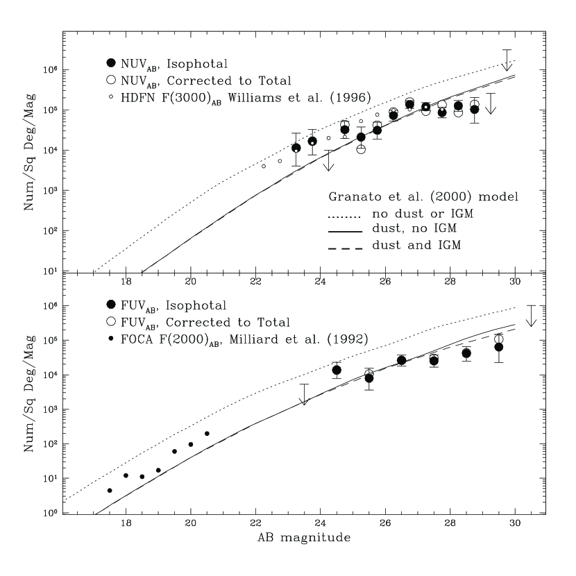
Figure 3: Galaxy counts. The large solid symbols are the isophotal counts, corrected for completeness as described in the text. The large open symbols have the magnitudes corrected to total. In the upper section of the Figure, we plot the WFPC2/F300W counts from Williams et al. (1996) and in the lower section we plot the balloon-based FOCA/2000Å counts of Milliard et al. (1992) for comparison. All counts are plotted in AB magnitudes, but we have not attempted to correct the comparison counts for the different bandpasses.