The ROSAT-ESO Flux Limited X-ray (REFLEX) Galaxy Cluster Survey II: The Spatial Correlation Function

Abstract

We report the results of the spatial two-point correlation function $\xi_{cc}(r)$ for the new X-ray galaxy cluster survey REFLEX, which comprises of 452 X-ray selected clusters (449 with redshifts) detected by the ROSAT satellite during the ROSAT All-Sky-Survey (RASS). The REFLEX cluster sample is flux limited to $3\times 10^{-12}$ erg s^-1 cm^-2 in the ROSAT energy band ($0.1-2.4$ keV) and spans 3 decades in X-ray luminosity ($10^{42}-10^{45}h^{-2}$ erg s^-1), containing galaxy groups and rich clusters out to a redshift $z\leq 0.3$. Covering a contiguous area of 4.24 sr REFLEX is the largest X-ray cluster sample to date for which spatial clustering has been analysed. Correlation studies using clusters selected on the basis of their X-ray emission are particularly interesting as they are largely free from the projection biases inherent to optical studies. For the entire flux-limited sample we find that the correlation length (the scale at which the correlation amplitude passes through unity) $r_{0}\simeq 20h^{-1}$Mpc. For example, if a power-law fit is made to $\xi(r)$ over the range $4-40h^{-1}$ Mpc then $r_{0}=18.8\pm 0.9$. An indication of the robustness of this result comes from the high degree of isotropy seen in the clustering pattern on scales close to the correlation length. On larger scales $\xi_{cc}(r)$ deviates from a power-law, crossing zero at $\simeq 45h^{-1}$ Mpc. From an examination of 5 volume-limited cluster sub-samples we find no significant trend of $r_{0}$ with limiting X-ray luminosity. A comparison with recent model predictions for the clustering properties of X-ray flux-limited samples, indicates that Cold Dark Matter models with the matter density $\Omega_{m}=1$ fail to produce sufficient clustering to account for the data, while $\Omega_{m}\simeq 0.3$ models provide an excellent fit.

1 INTRODUCTION

Clusters of galaxies have been used for many years as tracers of the large-scale mass distribution in the universe. As the largest gravitationally bound objects their clustering statistics provide important information on the hierarchical process of galaxy formation enabling estimates to be made of the mass fluctuation amplitude and the density paramter $\Omega$ (e.g. Mo et al. 1996). The early statistical analyses relied on the visual cluster compilations of Abell (1958) and Abell, Olowin & Corwin (1989). From the redshift surveys of richness-limited subsamples of the Abell catalogue (Bahcall & Soniera 1983, Klypin & Kopylov 1983, Postman et al. 1992, Peacock & West 1992) it was established that the correlation function $\xi_{cc}(r)$ followed the form

$$\xi_{cc}(r)=\left(\frac{r}{r_{0}}\right)^{-\gamma},$$ (1)

on scales $\leq 100h^{-1}$ Mpc with $\gamma\simeq 2$ and $r_{0}$ systematically 5 times higher than the value of $\simeq 5h^{-1}$ Mpc found for galaxies (e.g. Davis & Peebles 1983, Tucker et al. 1997), but with a strong dependency on the limiting richness of the cluster sample used (see Bahcall 1988). For example, while the richness class $R\geq 0$ samples give $r_{0}\simeq 20h^{-1}$Mpc, at the higher threshold $R\geq 2$ the correlation length rises to $r_{0}\simeq 40h^{-1}$Mpc (Peacock & West 1992). In principle these results can be used to place constraints on theoretical models of large-scale structure, however the cosmological information they contain is questionable due to the likely existence of inhomogeneities (Sutherland 1988, Sutherland & Efstathiou 1991) and line-of-sight projection effects (Lucey 1983, Dekel et al. 1990) artificially enhancing the correlation amplitude of Abell-based cluster samples. Strong evidence that these effects play a significant role comes from comparing the amplitude of the correlation function $\xi(\sigma,\pi)$ in the redshift direction $\pi$ of space with the perpendicular direction $\sigma$. Both rich and poor Abell cluster samples regularly fail this isotropy test, showing line-of-sight elongations in the contours of $\xi(\sigma,\pi)$. These features are consistent with an artificial enhancement of the correlation function (Sutherland 1988, Efstathiou et al. 1992, Peacock & West 1992) although physical interpretations have also been suggested (Bahcall et al. 1986, Miller et al. 1999).

The advent of digitised cluster surveys saw a dramatic increase in the homogeneity with which optical cluster samples could be compiled. Results from both the Edinburgh/Durham Cluster Catalogue (Nichol et al. 1992) and the APM survey (Dalton et al. 1992, 1994, Croft et al. 1997) demonstrated that for the equivalent Abell richness class $R\geq 0$, clusters found from automated detection algorithms have $r_{0}\simeq 15h^{-1}$Mpc with significantly reduced anisotropies. Testing the results of the richer clusters has proved more difficult due to the large search volume required to find suitable numbers and the diminishing contrast of distant clusters against the background of faint galaxies. For example, Croft et al. (1997) used 46 APM clusters with richnesses equivalent to $R\geq 2$ and found $r_{0}\simeq 20\pm 5$.

In recent years attention has focused on cluster samples generated on the basis of their X-ray emission. This method has enormous advantages for the determination of $\xi_{cc}$ over the optically compiled cluster catalogues described above:

• The X-ray emission from a cluster provides a direct physical link with the presence of a large gravitational potential in quasi-equilibrium (e.g. $L_{x}\propto M^{4/3}$). Thus the signature of X-ray emission provides strong evidence that the apparent overdensities seen in the optical are gravitationally bound structures.

• The emissivity of Thermal Bremsstrahlung radiation is proportional to the square of the electron number density, whereas the optical richness estimates are simply proportional to the galaxy density. Therefore, at fixed density, the contamination in cluster samples resulting from the projection of systems along the line-of-sight is intrinsically higher in richness-based optical samples compared to X-ray cluster catalogues. Furthermore the X-ray emission from clusters is concentrated towards the dense central cores which are typically $\sim 250h^{-1}$ kpc in size – significantly smaller than the spatial extent of the galaxy concentration in clusters. Both these effects substantially reduce the chance of projection effects which, as described above, are thought to plague Abell-based samples.

• The comparatively low internal background of the ROSAT Position Sensitive Proportinal Counter (PSPC) and the relatively short exposure times in the All-Sky Survey means that the X-ray fluxes from clusters at the flux limit of REFLEX are photon-noise limited as opposed to background limited. This is in contrast to purely optically selected samples which are forced to have a minimum density contrast above a varying background of galaxies before they can be detected.

The first attempts to measure $\xi_{cc}$ using X-ray clusters were confined to small samples: Lahav et al. (1989) detected significant clustering with $r_{0}\sim 21h^{-1}$ for $\gamma=1.8$ using an all-sky sample of 53 clusters above a flux $1.7\times 10^{-11}$ erg s^-1 cm^-2 (2-10 keV). Nichol, Briel & Henry (1994) used ROSAT data for a complete sample of 67 X-ray bright Abell clusters finding a correlation length $r_{0}=16.1\pm 3.4h^{-1}$ Mpc and detecting no significant clustering anisotropy. A more extensive study using data from the ROSAT satellite carried out by Romer et al. (1994) for a nearly complete flux-limited sample of 129 clusters above $1\times 10^{-12}$ erg s^-1 cm^-2 found $r_{0}=12.9\pm 2.2h^{-1}$Mpc, $\gamma=1.8\pm 0.4$. This study also found no evidence of spatial anisotropy in the clustering pattern. More recently, there have been two independent estimates of $\xi_{cc}$ from the 277 X-ray brightest Abell cluster sample from the RASS (XBACS, Ebeling et al. 1996). For this sample Abadi et al. (1998) suggest $r_{0}=21.1^{+1.6}_{-2.3}h^{-1}$Mpc and $\gamma=1.9$ from a $\chi^{2}$ minimisation procedure using the binned correlation data, while Borgani et al. (1999) use a more reliable likelihood analysis finding $r_{0}=26.0^{+4.1}_{-4.7}h^{-1}$ Mpc (here error bars are $2\sigma$). The anisotropy diagram for XBACS is published by Miller et al. (2000) and shows strong Abell-type elongations.

These X-ray results do not attempt to take account of the sky coverage of the parent X-ray survey in the correlation analysis. However, X-ray cluster samples generated from the RASS (Trümper 1993, Voges et al. 1999) have the advantage that the sky coverage is known from accurate information on the X-ray flux limit pertaining to any part of the sky.

The first attempt to utilise the RASS sky coverage information is Moscardini et. al. (2000a), who analyse the spatial distribution of the clusters in the RASS1 Bright Sample (De Grandi et al. 1999) using a very simple version of the sky coverage based on the first processing of the All-Sky Survey. This cluster catalogue is the forerunner to REFLEX consisting of 130 clusters to a limit $3-4\times 10^{-12}$ erg s^-1 cm^-2 defined in the ROSAT hard energy band ($0.5-2.0$ keV) and covering an area covering 2.5 sr centred on the Southern Galactic Cap. Moscardini et al. (2000a) find $r_{0}=21.5^{+3.4}_{-4.4}h^{-1}$ and $\gamma=2.1^{+0.53}_{-0.56}$ ($95.4\%$ errors) with a mild dependence of $r_{0}$ on limiting flux and luminosity. The REFLEX survey provides the opportunity to substantially improve on this result in a number of important respects: (i) REFLEX provides more than 3 times the number of X-ray clusters over a contiguous area nearly twice as large. (ii) All RASS standard analysis source detections are reanalysed using our own flux determination method. (iii) Due account is taken of all exposure variations, in contrast to the the RASS1 sample which is limited to exposure times larger than 150 secs. (iv) The optical identification is done in a homogeneous way based on the most comprehensive optical data base available for the southern sky. The power spectrum for REFLEX is presented elsewhere (Schuecker et al. 2000), here we concentrate on the correlation function.

The outline of the paper is as follows: In Section 2 we give a brief description of the REFLEX cluster survey. In Section 3 we discuss the algorithm used to esimate the the correlation function and the results for both the entire REFLEX catalogue and volume limited sub-samples are presented in Section 4. The interpretation of these results in terms of structure formation models is discussed in Section 5.

2 THE REFLEX Survey

The REFLEX survey represents an objective flux-limited catalogue of X-ray clusters in the southern hemisphere south of declination +2.5 degs and excluding the region within $\pm 20$ deg of the Galactic Plane. A further $\simeq 324$ deg² of sky around the LMC and SMC is removed where X-ray detection is hampered by the high interstellar absorption and crowded star fields. The remaining area covered by the survey is 13924 deg² or 4.24 sr, representing $\simeq 34\%$ of the entire sky.

The primary X-ray data for REFLEX originates from the second processing of the ROSAT All-Sky-Survey (RASS2) using the Standard Analysis Software System (SASS) which is based on a maximum likelihood detection algorithm. Confirmed RASS2 sources with a likelihood parameter of at least 15 and count rate $\geq 0.05$ cts s^-1 in the $0.1-2.4$ keV energy band have already been published in the RASS bright source catalogue (Voges et al. 1999). For REFLEX we use the internal MPE source catalogue totalling 54076 sources in the study area which allows the inclusion of sources with a likelihood $\geq 7$. Although some sources will be detected at a significance $\leq 3\sigma$ and not all are real, this lower likelihood threshold ensures that the parent catalogue is as complete as possible.

Figure 1: The sky coverage for REFLEX as a function of flux limit in the ROSAT energy band. The curve is determined from the satellite exposure map, the local hydrogen column density and the criterion that at least 10 photons are detected. The dashed vertical line shows that REFLEX reaches $3\times 10^{-12}$ erg s^-1 cm^-2 for $97.4\%$ of the survey.

It is well known from previous studies that the RASS analysis software is optimised for point-like sources and therefore underestimates the flux of extended sources (e.g. Ebeling et al. 1996, De Grandi et al. 1997). Therefore we have reanalysed all the source fluxes using a growth curve analysis method to recover the total flux of extended sources with an internal error of between $10-20\%$ (Böhringer et al. 2000a). Note: X-ray count rates are measured in the hard band ($0.5-2.0$ keV) then converted to unabsorbed fluxes in the ROSAT band ($0.1-2.4$ keV) and the cluster X-ray luminosities are determined by an iterative procedure using the luminosity-temperature relation of Markevitch (1998) assuming $h=0.5$ (Böhringer et al. 2000c in preparation), with the values scaled by a factor 0.25 to $h=1$ in this paper. Excluding double detections we have 4206 sources above a count rate limit of 0.08 cts s^-1, which corresponds to a flux limit between $1.6-2.0\times 10^{-12}$ erg s^-1 cm^-2.

The optical identification is based on finding galaxy overdensities in concentric rings around X-ray source positions using the UK Schmidt J-survey photographic plates digitised by COSMOS which reduces the total number of cluster candidates to $\simeq 500$ above a flux limit $3\times 10^{-12}$ erg s^-1 cm^-2 in the ROSAT energy band $0.1-2.4$ keV. Details of the optical identification process are given elsewhere (Böhringer et al. 2000b).

To carry out further indentification and obtain redshifts, multi-object ($5-20$ galaxies per cluster) and single-slit ($2-3$ galaxies per cluster) spectroscopy was carried out on $\simeq 431$ targets as part of an ESO Key Programme (Böhringer et al. 1998, Guzzo et al. 1999). This results in 452 clusters above $3\times 10^{-12}$ erg s^-1 cm^-2 in the energy band $0.1-2.4$ keV, of which 449 have secure redshifts either from our ESO programme or from the literature. About $65\%$ of these clusters are in the Abell catalogue while most of the others were previously unknown.

A comprehensive discussion of the contamination and completeness statistics in REFLEX is given in Böhringer et al. (2000b) and results on the comoving number density of clusters in the survey are presented in Schuecker et al. (2000). These indicate a completeness well in excess of $\geq 90\%$ and a contamination by non-cluster X-ray sources of less than $9\%$. We mention a few results here to serve as an illustration of the quality of the catalogue: (i) From a search for X-ray emission around all ACO and ACO supplimentary clusters only 1 cluster with an X-ray flux more than the flux limit is not found by the selection process. (ii) Clusters in the luminosity range $0.08-2.5\times 10^{44}h^{-2}$ erg s^-1 have a constant comoving number density of objects and V/Vmax=$0.51\pm 0.01$ at the flux limit of the survey. This is consistent with the lack of evolution seen in the X-ray luminosity function out to at least $z\simeq 0.3$ reported by other surveys (e.g. Burke et al. 1997, Ebeling et al. 1997). (iii) Approximately $81\%$ of the REFLEX clusters are extended – we searched the RASS2 database separately for extended X-ray sources finding only a further 8 bona-fide clusters and 5 candidate clusters, 3 of which show no obvious optical counterpart and for which futher deep imaging is planned.

3 Calculating the correlation function

3.1 Areal Coverage

One complication with the RASS is that the sky coverage is not homogeneous resulting in about $12\%$ of the REFLEX survey region having an exposure time less than half of the median exposure time ($\simeq 323$ s). This, coupled with the varying galactic hydrogen coloumn density, results in a variation of the limiting flux of the RASS2 across the sky. Although the very low background for the ROSAT PSPC, especially in the hard band ($0.5-2.0$ keV), allows the detection and characterisation of sources with comparitavely low source source counts a minimum number is required for a safe detection. Fig. 1 shows the resulting effective area of the REFLEX survey as a function of flux with the additional criterion imposed of detecting at least 10 photons in the hard band. The exposure times of the RASS2 in the REFLEX area are sufficient that at a flux limit of $3\times 10^{-12}$ erg s^-1 cm^-2 at least 10 photons are detected for $97.4\%$ of the REFLEX survey area and hence the number of clusters detected with low photon counts is very small – 3.8 clusters with less than 10 counts are expected in the survey and only 1 is detected. For a more conservative requirement of at least 30 photons for each source the sky coverage falls to $78\%$ (see Böhringer et al. 2000b).

3.2 Correlation Estimator

In all computations we use the estimator

$$1+\xi_{cc}(r)=4\frac{(DD)(RR)}{(DR)^{2}},$$ (2)

where DD stands for the number of distinct pairs in the data, RR stands for the number of distinct pairs in the random catalogue and DR represents the number of cross pairs. The factor of 4 in this expression accounts for the fact that while the number of distinct pairs in a large catalogue of size $n$, say, is $\simeq n^{2}/2$, the number of cross-pairs between two different catalogues each with $n$ entries is $\simeq n^{2}$ and these are all distinct. Since the correlation function is defined in terms of the total number of pairs, the number of distinct $DD$ and $RR$ pairs must each be multiplied by 2 to obtain the total numbers, hence the factor of 4. This estimator has been shown by Hamilton (1993) to be the most robust for datasets which may be sensitive to the chance location of strong clustering close to the sample boundary.

In principle the estimator in equation 2 can be generalised to include an arbitrary weighting function. For calculating the correlation function of galaxies from magnitude-limited samples, the variance in the estimate of $\xi(r)$ on large scales is minimised if $w(r_{i},\tau)$ is

$$w(r_{i},\tau)=\frac{1}{1+4\pi n_{D}J_{3}(\tau)\phi(r_{i})},$$ (3)

where $r_{i}$ is the distance of an object from the origin, $\tau$ is the distance separating two objects, $\phi(r)$ is the survey selection function, $n_{D}$ the mean space density of objects and $J_{3}(\tau)=\int_{0}^{\tau}drr^{2}\xi(r)$ (see Saunders, Rowan-Robinson & Lawrence 1992, Fisher et al. 1994, Guzzo et al. 2000). The physical interpretation of the term $4\pi n_{D}J_{3}(\tau)$ in the weighting scheme is that it represents something like ‘the mean number of objects per clump’. For galaxies this number is large on small scales giving equal volume weighting to the pairs ($w\propto 1/\phi(r)$). By contrast, for clusters the weighting term $4\pi n_{D}J_{3}(\tau)$ is always small compared to unity on scales of interest and consequently we assign equal weight to all pairs in the calculation of the cluster correlation function.

We calculate spatial separations using the formula for comoving coordinate distance ($r_{1}$);

$$r_{1}=\frac{\rm{c}}{\rm{H}_{0}}\left[\frac{(q_{0}z)+((1-q_{0})(1-((2q_{0}z)+1)^{1/2}))}{(1+z)q^{2}_{0}}\right],$$ (4)

adopting the cosmology $\rm{H}_{0}=100h^{-1}$ Mpc, $\Omega_{m}=1.0$ & $\Omega_{\Lambda}=0.0$, along with the cosine rule to determine angular separations.

3.3 Random catalogues

The random catalogues are constructed over the REFLEX survey area using a Monte-Carlo technique which incorporates knowledge of the flux limit in cells of size $\simeq 1$ square degree. To begin with it is assumed that the observed number count distribution of X-ray clusters, LogN-LogS, is well fitted by a simple lower-law:

$$N(>S)=AS^{-\alpha}.$$ (5)

For the purposes here we adopt the value $\alpha=1.35$, consistent with the REFLEX number counts (see Böhringer et al. 2000b) and those of RASS1, the precursor survey of REFLEX (De Grandi et al. 1999). Small changes to the value of $\alpha$ does not alter the outcome of the results. If we assume that the accumulative distribution $P$ defined as

$$\frac{N(<S)}{N_{total}(>S_{lim})}=P$$ (6)

is uniformly distributed in the range $0\rightarrow 1$, then the distribution of cluster X-ray fluxes $S$ selected at random above $S_{lim}$ is given by

$$S=S_{lim}(1-P)^{-\frac{1}{\alpha}}.$$ (7)

Figure 2: Aitoff plot of 449 REFLEX Clusters with redshift.

Figure 3: Aitoff plot of 1000 random points generated with the REFLEX sensitivity map (flux limit $3\times 10^{-12}$ erg s^-1 cm^-2 with a minimum of 10 photon counts) and mask.

We select a cluster at random within the allowed borders of the REFLEX survey and then use eqn. 7 to assign it a flux. We then test whether the cluster falls above or below the flux limit for that region of the REFLEX survey based on the local values of exposure time and the interstellar hydrogen column density (Dickey & Lockman 1990, Stark et al. 1992). We set $S_{lim}=3\times 10^{-12}$ erg s^-1 cm^-2, which is the cut-off flux limit for the entire survey. An example of a random catalogue with 1000 points generated in this way is shown in Fig. 3. To demonstrate reliability of the random catalogues the histogram in Fig.  4 shows the number of REFLEX clusters as a function of Galactic longitude and latitude compared to that of a random catalogue generated using the REFLEX survey sensitivity map. The random catalogues used in the determination of $\xi_{cc}$ contain typically 100,000 points.

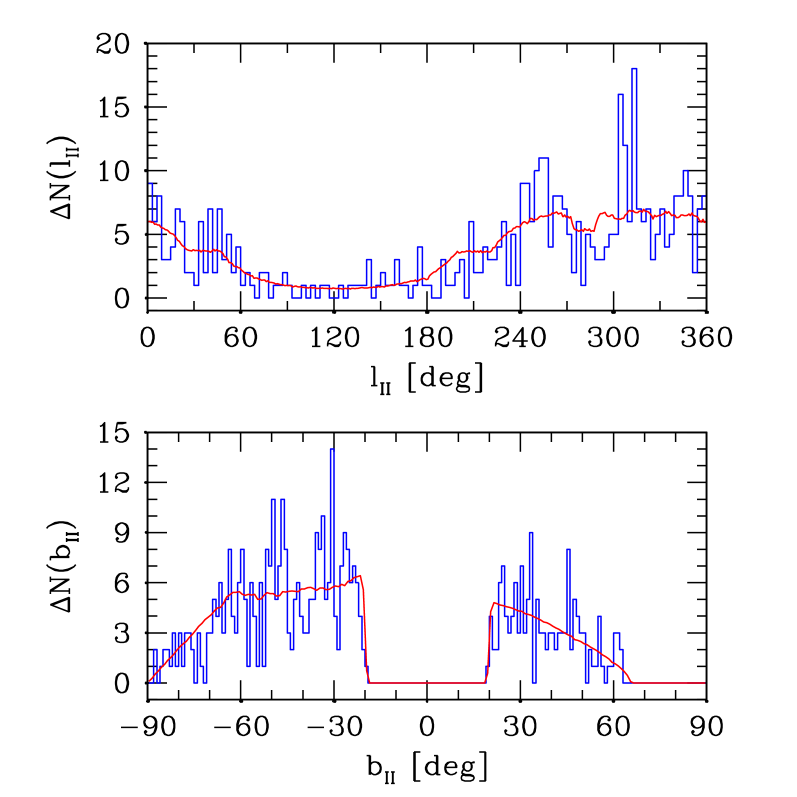
Figure 4: Histogram of REFLEX clusters as a function of galactic longitude and latitude. The solid line is the prediction from a random distribution of points convolved with the REFLEX sensitivity map (flux limit $3\times 10^{-12}$ erg s^-1 cm^-2 with a minimum of 10 photon counts) and mask.

Figure 5: Histogram of the 449 REFLEX clusters with redshifts. The solid line is the estimated density distribution using a Gaussian kernel of width 5600 km s^-1.

Figure 6: Histogram of the 399 REFLEX clusters with $L_{x}\geq 3\times 10^{44}$ erg s^-1. The dashed curve is the estimated redshift distribution of this sample using a Gaussian kernel of width 5600 km s^-1, as for Fig. 5. The solid curve is the redshift distribution estimated by integrating the X-ray cluster luminosity function.

We use two methods to assign each random point a redshift. (i) Redshifts are drawn from the distribution of REFLEX clusters smoothed with a Gaussian kernel. This method allows the redshift selection function to be estimated without prior knowledge of the underlying density distribution of clusters and is used in almost all previous determinations of the cluster correlation function. For REFLEX we use a Gaussian of width 5600 km s^-1 – the optimum value depends on the space density of clusters and is constrained by the need to follow the redshift distribution accurately enough while not removing large-scale clustering. The exact figure used is generally not critical, with values in the literature ranging between $4000-8000$ km s^-1. (ii) The second method, which we apply to luminosity limited samples, uses the X-ray cluster luminosity function to generate the expected number of clusters at each redshift. Assuming a Schechter function of the form

$$n(L)dL=Aexp(L/L_{\star})(L/L_{\star})^{-\alpha}dL,$$ (8)

where $n(L)$ is the number density of clusters per luminosity interval, then for particular values of $\alpha$ and $L_{\star}$, we can integrate $n(L)dL$ above $L_{lim}$ to determine the number density of clusters at each redshift $\eta(z)$. The value of $L_{lim}$ at each redshift is found from the flux limit (fixed at $3\times 10^{-12}$erg s^-1 cm^-2). The expected number of clusters in each redshift interval $dz$ is then simply $\eta(z)*dV(z)$, where $dV(z)$ is the comoving volume element at redshift $z$. Each random point generated in the area of the survey is thus assigned a random redshift weighted by the expected number of clusters based on eqn. 8. We have used the values of $\alpha=1.61$, $L_{\star}=6.04\times 10^{44}$ (erg s^-1), $A=3.04\times 10^{-8}$ ($10^{44}$ erg s${}^{-1})^{-1}$ and H${}_{0}=50$ km s^-1 Mpc^-1, which are appropriate to the REFLEX sample (Böhringer et al. 2000c, in preparation), although using our previous luminosity function parameters from De Grandi et al. (1999) gives identical results. The redshift distribution for the REFLEX sample along with the smoothed version using method (i) is shown in Fig. 5, while Fig. 6 shows a comparison between the redshift distribution of both methods for the luminosity subsample of 399 clusters limited to $L_{x}\geq 3\times 10^{44}$erg s^-1. We prefer method (ii) for the luminosity sub-samples as it makes no prior assumptions regarding the scale of the clustering and avoids the need to smooth the data, however in practice we found no significant difference in the correlation functions resulting from the two methods.

3.4 Maximum Likelihood Determination of $r_{0}$ and $\gamma$

In calculating the best-fit power-law for the correlation function from samples of $\sim 100$ clusters there has traditionally been one of two methods adopted. The first is to calculate errors for $\xi_{cc}$ based on estimates from pair counts binned into $\simeq$ 10 coarse intervals, which are usually spaced logarithmically out to $\simeq 100h^{-1}$ Mpc (e.g. Bahcall et al. 1983, Dalton et al. 1992, Nichol et al. 1992). On the grounds that each bin contains a large numbers of pairs, the best-fit power-law is estimated using the $\chi^{2}$ statistic. The danger with such an approach is that the resulting estimates of parameters describing the power-law ($r_{o},\gamma$) will then depend on the precise details of the binning. In order to overcome this limitation we adopt the second of the two methods referred to above and maximise the likelihood $L$ that the model correlation function produces the measured number of cluster pairs at a given separation (Croft et al. 1997, Borgani et al. 1999, Moscardini et al. 2000a). The likelihood estimate is based on Poisson probabilities, such that

$$L=\prod_{i=1}^{N}e^{-\mu}\mu^{\nu}/\nu!,$$ (9)

where $\nu$ is the observed number of cluster-cluster pairs in a small interval $dr$ and $\mu$ is the expected number in the same interval calculated using Hamilton’s estimator (eqn. 2). As long as the number of random points is kept large enough to avoid a zero in the denominator of eqn. 2, $dr$ can be made arbitrarily small, so as to ensure the final results are independent of the bin size. In practice we used $\sim 7000$ bins between $5-100$ Mpc, which resulted in either a 0 or 1 cluster-cluster pair in almost all bins.

The associated errors on the correlation function are usually calculated from ‘Poisson’ statistics. In the case of large bin intervals errors are computed from the formula

$$\delta\xi_{cc}(r)=\frac{(1+\xi_{cc}(r))}{\sqrt{N_{cc}}},$$ (10)

where $N_{cc}$ is the number of distinct cluster pairs in the bin centred at separation $r$. In the case of a maximum likelihood determination, such as that used here, confidence levels can be defined as $S(r_{best},\gamma_{best})-S(r_{0},\gamma)$, where $S$ is the usual $S=-2lnL$, assuming that $\Delta S$ is distributed like $\chi^{2}$.

Both these methods are likely to produce underestimates of the true dispersion as the use of Poisson statistics assumes that the pair counts are independent of each other, which is clearly not the case. An estimate of the true dispersion in the correlation function, which tries to account for cosmic variance, can be made either by applying a bootstrap resampling of the real data (e.g. Ling, Frenk & Barrow 1986; Mo, Jing & Börner 1992) or by carrying out numerical simulations based on plausible cosmological models (Croft & Efstathiou 1994, Croft et. al. 1997). Both methods produce similar results indicating that the real errors are probably $1-2$ times larger than the Poisson-based estimates. We confirmed this result for our sample by generating mock catalogues from bootstrap resampling of the data and calculating the best-fit $r_{0}$ and $\gamma$ values using the likelihood method described above. The ratio of the error for $r_{0}$ from the variance between the bootstrap samples and the Poisson error is between $\simeq 1.5-2.0$ for all luminosity subsamples. Unless stated otherwise, in the results which follow we quote the $1\sigma$ likelihood errors on the values of $r_{0}$ and $\gamma$.

4 Results

Figure 7: The correlation function for the REFLEX survey of 449 clusters. The error bars on each point are derived from bootstrap statistics. The solid line shows the result of the likelihood analysis ($r_{0}=18.8$, $\gamma=1.83$) fitting a power law over the range $4-40h^{-1}$ Mpc.

Figure 8: The probability contours ($1\sigma,2\sigma,3\sigma$) for the best fit $r_{0}$ and $\gamma$ from the likelihood analysis of the REFLEX survey over the range $4-40h^{-1}$ Mpc.

Figure 9: The X-ray luminosity ($0.1-2.4$ keV) vs redshift for the REFLEX sample of 449 clusters. Also shown are the 5 volume complete sub-samples used to examine the variation of the correlation length with limiting X-ray luminosity ($L_{lim}$.

The $\xi_{cc}(r)$ for the REFLEX survey of 449 clusters is shown in Fig. 7. A fit was made to the correlation function assuming a single power law over the range $4-40h^{-1}$ Mpc using the likelihood analysis described in Section 3.4. Fig. 8 shows the corresponding joint constraints resulting from this analysis. The best-fit value for the power-law parameters are $r_{0}=18.8\pm 0.9$ and $\gamma=1.83^{+0.15}_{-0.08}$. If points are included on larger scales then the slope steepens, e.g. fitting between $4-100h^{-1}$ Mpc gives $\gamma\simeq 2.35$ and $r_{0}\simeq 16.25$. The inability of a single power law to adequately describe the correlation function is further reflected in the zero crossing of $\xi_{cc}$ at $45h^{-1}$ Mpc (see Section 7.1).

In order to investigate the dependency of $r_{0}$ with X-ray luminosity we also calculated $\xi_{cc}(r)$ for 5 volume-limited X-ray sub-samples with luminosity thresholds $0.08,0.18,0.3,0.5,1.0$ in units of $10^{44}h^{-2}$ erg s^-1. Fig. 9 shows the distribution of luminosity with redshift for the REFLEX sample along with the regions corresponding to the 5 subsamples. Due to the significant covariance between $r_{0}$ and $\gamma$ this investigation has been carried out with $\gamma$ fixed at 2.0. The correlation results for the sub-samples are presented in Table 1 and Fig. 10. These indicate no significant positive trend of $r_{0}$ vs $L_{lim}$, with the highest measured $r_{0}$ occuring at intermediate luminosities ($L_{lim}\geq 0.3\times 10^{44}h^{-2}$ Mpc). Beyond this point the statistical errors increase rapidly. To test the reliability of the parameter $r_{0}$ as an indicator of how clustering changes with X-ray luminosity, we calculated the average correlation function amplitude for the 5 volume-limited sub-samples over the range of separations $0-20h^{-1}$ Mpc. The result, shown in Fig. 11, is in good agreement with the trend of $r_{0}$ vs $L_{lim}$.

Table 1: Estimates of r₀ as a function of limiting X-ray luminosity for volume limited cluster subsamples. Values of r₀ are calculated at $\gamma=2.0$

$L_{lim}(10^{44}h^{-2}$) erg s -1	Number	$r_{0}$
1.0	67	$22.9^{+7.3}_{-7.7}$
0.5	101	$25.8^{+3.2}_{-3.3}$
0.3	108	$31.1^{+2.0}_{-2.1}$
0.18	84	$25.8^{+1.9}_{-2.0}$
0.08	39	$24.8^{+2.5}_{-2.5}$

Figure 10: The correlation function amplitude $r_{0}$ plotted against limiting X-ray luminosity defined in the ROSAT energy band ($0.1-2.4$ keV). The errors correspond to $1\sigma$ from the likelihood analysis.

Figure 11: The correlation function amplitude in the range $0-20h^{-1}$ Mpc plotted against limiting X-ray luminosity defined in the ROSAT energy band ($0.1-2.4$ keV). The error bars are $1\sigma$ based on eqn. 10.

Figure 12: Contours of constant $\xi(\sigma,\pi)$ for the REFLEX survey. The contour values used are 4.0, 2.0, 1.0 and then 0.8 to -0.4 in steps of 0.2

We have examined the isotropy of the clustering signal for the REFLEX survey by plotting contours of $\xi(\sigma,\pi)$, where $\pi=|r_{1}-r_{2}|$ is the line-of-sight separation, with $r_{1,2}$ determined from eqn. 4, and $\sigma=(s^{2}-\pi^{2})^{1/2}$ is the perpendicular component of the cluster separation $s$. As discussed in the introduction, elongations of the contours in the redshift direction compared to the perpendicular direction for scales $\simeq 20h^{-1}$) Mpc are a feature of some optical cluster catalogues – typically with a ratio $\simeq 4:1$ for redshift samples based on the Abell catalogue (e.g. Postman et al. 1992). Fig. 12 represents the corresponding plot for the REFLEX clusters and indicates that unlike optical surveys, the $\xi(\sigma,\pi)$ contours are close to being completely concentric on scales close to the correlation length.

5 Discussion

The determination $\xi_{cc}$ from the REFLEX survey can be compared with similar determinations for other X-ray cluster samples. Our results of $r_{0}=18.8$ and little dependency of $r_{0}$ on X-ray luminosity are broadly consistent with the results of XBACS (Borgani et al. 1999) and RASS1 (Moscardini et al. 2000a). The result presented by Romer et al. (1994), hereafter R94, for a sample of 128 clusters above $1.0\times 10^{-12}$ erg s^-1 cm^-2 in a 3100 deg² area centered on the SGP, suggests a correlation length $r_{0}=13-15h^{-1}$ Mpc, smaller than any of the other determinations from X-ray samples. In addition to the fainter flux limit, the R94 study differs from REFLEX in 2 further ways which in principle could affect the result: (i) the cluster sample was based on a reduction of the all-sky-survey using the ROSAT Standard Analysis Software, which has subsequently been revised (ii) the correlation analysis performed by R94 did not include the sample sky coverage corresponding to the SGP region under study. We have investigated the origin of a possible systematic difference between R94 and REFLEX by repeating our correlation analysis on the 109 REFLEX clusters lying within the R94 SGP area of sky, defined by the boundaries $22\rm{hr}\leq\rm{RA}\leq 3\rm{hr}$, $-50^{\circ}\leq\rm{dec}\leq 2^{\circ}$,$|b|\geq 40^{\circ}$. The resulting power-law fit to the correlation function out to $\leq 100h^{-1}$ Mpc gives $r_{0}=12.9^{+1.9}_{-1.9}$ $\gamma=2.0^{+0.4}_{-0.4}$, smaller than the REFLEX amplitude of $18.8\pm 0.9$ and very close to the original SGP result of $r_{0}=12.9\pm 2.2\,h^{-1}$ Mpc, $\gamma=1.8\pm 0.4$ found by R94 fitting over the same range. This suggests that the difference between the REFLEX and the SGP result is most likely due to the superior statistical sampling of REFLEX which represents a 4-fold increase in survey area over the SGP region while probing to a similar redshift.

Miller et al. (2000) analyse the $\xi(\sigma,\pi)$ diagram for a number of X-ray cluster samples. In their analysis the XBACS clusters show very strong elongations around $\xi(\sigma,\pi)\simeq 1$ in the redshift direction and a similar anisotropy is present in other X-ray confirmed Abell cluster samples. The RASS1 sample shows a much weaker anisotropy over the same scale. On the basis of this Miller et al. (2000) argue that clustering anisotropy is a ubiquitous feature of X-ray cluster samples which demonstrates that the anisotropies are real. However, the absence of any significant anisotropy in the contours of $\xi(\sigma,\pi)$ for the REFLEX survey shown in fig. 12 indicates that this is not the case. This is the strongest indication yet that elongations seen in other catalogues are spurious and justifies the claim, first pointed out by R94, that X-ray selected surveys do not suffer from significant projection biases. As with optical studies based on the Abell catalogue, the presence of strong elongations close to the scale of $r_{0}$ in the XBACS bring the accuracy of the clustering signal derived from this sample into question.

5.1 Comparison with Cosmological Models

Figure 13: The REFLEX correlation function compared with a range of Cold Dark Matter models for which $\Omega_{m}=1$ and $\Omega_{\Lambda}=0$, using the same flux limit and sky coverage as REFLEX – taken from Moscardini et al. (2000b). Error bars in this figure are $1\sigma$ and based on bootstrap resampling.

Figure 14: The REFLEX correlation function as for Fig. 13 but compared with two open CDM models for which $\Omega_{m}=0.3$, $\Omega_{\Lambda}=0.0$ (OCDM) and $\Omega_{m}=0.3$, $\Omega_{\Lambda}=0.7$ ($\Lambda$CDM), also from Moscardini et al. (2000b).

Figure 15: Comparison of the REFLEX correlation length $r_{0}$ from the likelihood analysis with predictions as a function of limiting X-ray flux for a range of CDM-type cosmological models (see text for details). The REFLEX point is plotted at $3\times 10^{-12}$ erg s^-1 cm^-2. The likelihood error bar of $0.9$ on $r_{0}$ has been increased by a factor 1.5 to 1.35 here to account for the extra contribution due to cosmic variance as described in Section 3.4.

Figure 16: The REFLEX correlation function at low amplitude. The error bars are calculated from eqn. 10. Also shown is the best power-law fit over the range $4-40h^{-1}$ Mpc corresponding to $r_{0}=18.8$ and $\gamma=1.83$. Predictions for the open and $\Lambda$-dominated CDM models from Moscardini et al. (2000b) are also presented.

Predictions for the clustering properties of X-ray selected clusters from a number of surveys, including REFLEX, have recently been made by Moscardini et al. (2000b). In these predictions the structures on a given scale are assumed to evolve by hierarchical merging of smaller units and instantaneous merging on cluster scales. The comoving mass function of haloes is computed using the Press-Schechter (1974) technique but incorporating more recent corrections which improve the comparison of Press-Schechter with numerical simulations (e.g. Sheth & Tormen 1999). The link between X-ray luminosity and mass of the hosting dark matter halo begins with the empirical relation between gas temperature $T$ and X-ray luminosity $L_{bol}$

$$T=AL^{\beta}_{bol}(1+z)^{-\nu},$$ (11)

with $A=4.2$ & $\beta=1/3$, which is a good approximation for clusters (e.g. David et al. 1993; White, Jones & Forman 1997; Markevitch 1998). The parameter $\nu$ describing the evolution of the $T-L_{bol}$ relation is constrained by Moscardini et al. (2000b) using the X-ray cluster number counts over the range $5\times 10^{-13}-3\times 10^{-11}$ erg s^-1 cm^-2 ($0.5-2.0$ keV) taken from the RASS1 Bright Sample (De Grandi et al. 1999) and the fainter ROSAT Deep Cluster Survey Rosati et al. (1998). It is possible to convert the temperature estimates from eqn. 11 to halo mass assuming a virial isothermal gas distribution and spherical collapse (e.g. Eke, Cole & Frenk 1996). Finally, in order to make predictions for the correlation function of the REFLEX survey, Moscardini et al. (2000b) incorporate the actual sky coverage of the survey shown in Fig. 1 for the passband $0.1-2.4$ keV in an identical manner to the procedure used for calculating $\xi_{cc}(r)$ using the REFLEX data described in Section 3.1 above.

The behaviour of the cluster correlation function for a range of popular cosmological models based around cold dark matter (CDM) are shown in Fig. 13 and Fig. 14. The model predictions are taken directly from Moscardini et al. (2000b) and represent: Standard (SCDM), $\tau$ ($\tau$CDM) and tilted (TCDM) models, all with $\Omega_{m}=1$ and $\Omega_{\Lambda}=0.0$; along with an open model $\Omega_{m}=0.3$ (OCDM) and a $\Lambda$-dominated model with $\Omega_{m}=0.3$ and $\Omega_{\Lambda}=0.7$. An examination of these figures reveals clear evidence for an inconsistency between all $\Omega_{m}=1$ models and the REFLEX correlation function, with a significantly better fit to the data for open or $\Lambda$-dominated cosmologies. This is further illustrated in Fig. 15 which shows the Moscardini et al. (2000b) predictions of correlation length with limiting X-ray flux. While the Einstein-de Sitter models predict $r_{0}=11-13h^{-1}$Mpc, both the OCDM and $\Lambda$CDM models predict $r_{0}\simeq 20h^{-1}$Mpc. These results are in agreement with the analysis of the X-ray clusters based on the RASS1 Bright Sample (Moscardini et al. 2000a) and the digitised optical surveys (e.g. Croft et al. 1997).

Confirmation of the general conclusions on the form of the cosmological power spectrum comes from the behaviour of of $\xi_{cc}$ on large scales. In Fig.  16 we show the REFLEX $\xi_{cc}(r)$ at low amplitude which shows a positive clustering signal out to at least $40h^{-1}$ Mpc ($\xi(30-40)=0.32\pm 0.08$), with a zero-crossing $\simeq 45h^{-1}$ ($\xi(40-50)=-4.7\times 10^{-3}\pm 0.05$). On larger scales the amplitude remains slightly negative ($\xi(50-100)=-0.07\pm 0.02$). Also shown is the curve representing the power law with $r_{0}=18.8h^{-1}$ Mpc and $\gamma=1.83$, along with predictions from Moscardini et al. (2000b) for the OCDM and $\Lambda$CDM models. Since the SCDM model predicts a zero-crossing near $r\simeq 33h^{-1}$Mpc (Klypin & Rhee 1994), the REFLEX data again support the findings of other cluster surveys that models with more power than SCDM are required to adequately fit the large-scale $\xi_{cc}(r)$. Generally for CDM-like models (with $n=1$ for the primordial spectral index) the first zero-point occurs at $r\simeq 16.5(\Omega_{m}h^{2})^{-1}$ for a vanishing baryon fraction (see Klypin & Rhee 1994). For the particular parameterisation used by Moscardini et al. (2000b) the OCDM and $\Lambda$CDM models remain positive until $\simeq 80h^{-1}$ Mpc, however the small clustering amplitude in the data between $\simeq 45-100h^{-1}$ Mpc seen in Fig. 16 prohibits any definitive comparison of the zero crossings.

6 Summary

Catalogues of galaxy clusters based on their X-ray emission provide a powerful tool for studies of large-scale structure. We present the spatial correlation function of the REFLEX cluster survey, which consists of 449 X-ray emitting clusters above a flux limit $3\times 10^{44}$ erg s^-1 cm^-2 and covering a contiguous area of 4.24 sr in the southern hemisphere. The advantages of X-ray selection, combined with the increased statistics and high completeness of REFLEX enable a significant step to be taken in establishing the clustering properties of clusters in the local universe. Over the scale $4-40h^{-1}$ Mpc we find a correlation amplitude $r_{0}=18.8\pm 0.9$ and power law index $\gamma=1.83^{+0.15}_{-0.08}$ for the entire survey. The high degree of isotropy in the correlation function demonstrates that systematic projection effects are not present in the data. By analysing volume-limited sub-samples we find no significant trend of clustering amplitude with X-ray luminosity. Comparing the REFLEX $\xi_{cc}$ results with predictions from various CDM-type models which incorporate directly the areal coverage of REFLEX, $\Omega_{m}\simeq 0.3$ models provide an excellent fit, while $\Omega_{m}=1$ & $\Omega_{\Lambda}=0$ models fail to provide enough large-scale power. Finally, it is intriguing to note the concensus emerging between clustering studies and the lack of evolution in the abundance of X-ray clusters (e.g. Burke et al. 1997, Collins et al. 1997, Borgani et al. 1999, Henry 1997, Nichol et al. 1999), which also indicates that the Einstein de-Sitter universe is in trouble.

REFERENCES

Abadi, M., Lambas, D., Muriel, H., 1998, ApJ., 507, 526

Abell, G.O., 1958, ApJS, 3, 211

Abell, G.O., Corwin, H.G., Olowin, R.P., 1989, ApJS, 70, 1

Bahcall, N.A., 1988, ARA&A, 26, 631

Bahcall, N.A., Soneira, R.M., 1983, ApJ., 270, 20

Bahcall, N.A., Soniera, R.M., Raymond, M., Burgett, W.S., 1986, ApJ, 113, 15

Böhringer, H., Guzzo, J., Collins, C.A., Neumann, D.M., Schindler, S., Schuecker, P., Cruddace, R.G., De Grandi, S., Chincarini, G., Edge, A.C., MacGillivray, H.T., Shaver, P., Vettolani, G., Voges, W., 1998, The Messenger, No. 94, 21

Böhringer, H., Voges, W., Huchra, J.P., McLean, B., Giacconi, R., Rosati, P., Burg, R., Mader, J., Schuecker, P., Simic, D., Komossa, S., Reiprich, T.H., Retslaff, J., Trümper, J., 2000, ApJ, submitted 2000a (astro-ph/0003219)

Böhringer, H., Schuecker, P., Guzzo, L., COllins, C.A., Voges, W., Schindler, S., Neumann, D.M., Chincarini, G., Cruddace, R.G., De Grandi, S., Edge, A.C., MacGillivray, H.T., Shaver, P., 2000, A&A, submitted 2000b Paper I

Borgani, S., Plionis, M., Kolokotronis, V., 1999, MNRAS, 305, 866

Borgani, S., Rosati, P., Tozzi, P., Norman, C., 1999, ApJ., 517, 40

Burke, D.J., Collins, C.A., Sharples, R.M., Romer, A.K., Holden, B.P., Nichol, R.C., 1997, ApJ, 488, L83

Collins, C.A., Burke, D.J., Romer, A.K., Sharples, R.M., Nichol, R.C., 1997, ApJ, 479, L117

Croft, R.A.C., Efstathiou, G., 1994, MNRAS, 267, 390

Croft, R.A.C., Dalton, G.B., Efstathiou, G., Sutherland, W.J., Maddox, S.J., 1997, MNRAS, 291, 305

Dalton, G.B., Efstathiou, G., Maddox, S.J., Sutherland, W.J., 1992, ApJ., 424, L1

Dalton, G.B., Croft, R.A.C., Efstathiou, G., Sutherland, W.J., Maddox, S.J., Davis, M., 1994, MNRAS, 271, 47

David, L.P., Slyz, A., Jones, C., Forman, W., Vrtilek, S.D., Arnaud, K.A., 1993, ApJ., 412, 479

Davis, M., Peebles, P.J.E., 1983, ApJ, 267, 465

De Grandi, S., Molendi, S., Böhringer, H., Chincarini, G., Voges, W., 1997, ApJ, 486, 738

De Grandi, S., Guzzo, L., Böhringer, H., Molendi, S., Chincarini, G., Collins, C., Cruddace, R., Neumann, D., Schindler, S., Schuecker, P., Voges, W., 1999, ApJ, 513, 17

Dekel, A., Bertschinger, E., & Faber, S.M., 1990, ApJ., 364, 349

Dickey, J.M., Lockman, F.J., 1990, ARAA, 28, 215

Ebeling, H., Voges, W., Böhringer, H., Edge, A.C., Huchra, J.P., Briel, U.G., 1996, MNRAS, 281, 799

Ebeling, H., Edge, A.C., Fabian, A.C., Allen, S.W., Crawford, C.S., Böhringer, H., 1997, MNRAS, 479, 101

Efstathiou, G., Dalton, G.B., Sutherland, W.J., Maddox, S.J., 1992, MNRAS, 257, 125

Eke, V.R., Cole, S., Frenk, C.S., 1996, MNRAS, 282, 263

Fisher, K.B., Davis, M., Strauss, M.A., Yahil, A., Huchra, J., 1994, MNRAS, 266, 50

Guzzo, L., Böhringer, Schuecker, P., Collins, C.A., Schindler, S., Neumann, D.M., De Grandi, S., Cruddace, R.G., Chincarini, G., Edge, A.C., Shaver, P., Voges, W., 1999, The Messenger, No. 95, 27

Guzzo, L., Bartlett, J.G., Cappi, A., Maurogordato, S., Zucca, E., Zamorani, G., Balkowski, C., Blanchard, A., Cayatte, V., Chincarini, G., Collins, C.A., Maccagni, D., MacGillivray, H., Merighi, R., Mignoli, M., Proust, D., Ramella, M., Scaramella, R., Stripe, G.M., Vettolani, G., 2000, A&A, 355, 1

Hamilton, A.J.S., 1993, ApJ., 406, L47

Henry, J.P., 1997, ApJ, 489, L1

Klypin, A., Kopylov, A.I., 1983, Sov. Astron. Lett., 9, 41

Klypin, A., Rhee, G., 1994, ApJ, 428, 399

Lahav, O., Edge, A.C., Fabian, A.C., Putney, A., 1989, MNRAS, 238, 881

Ling, E.N., Frenk, C.S., Barrow, J.D., 1986, MNRAS, 223, L21

Lucey, J.R., 1983, MNRAS, 204, 33

Markevitch, M., 1998, ApJ., 504, 27

Miller, C.J., Batuski, D.J., Slinglend, K.A., Hill, J.M., 1999, ApJ., 523, 492

Miller, C.J., Ledlow, M.J., Batuski, D.J., 2000, MNRAS, submitted (astro-ph/9906423)

Mo, H.J., Jing, Y.P., Börner, G., 1992, ApJ., 392, 452

Mo, H.J., Jing, Y.P., White, S.D.M., 1996, MNRAS, 282, 1096

Moscardini, L., Matarrese, S., De Grandi, S., Lucchin, F., 2000, MNRAS, in press (2000a)

Moscardini, L., Matarrese, S., Lucchin, Rosati, P., 2000, MNRAS, in press(2000b)

Nichol, R.C., Briel, O.G., Henry, P.J., 1994, ApJ., 267, 771

Nichol, R.C., Collins, C.A., Guzzo, L., Lumsden, S.L., 1992, MNRAS, 255, L21

Nichol, R.C., Romer, A.K., Holden, B.P., Ulmer, M.P., Pildis, R.A., Adami, C., Merrelli, A., Burke, D.J., Collins, C.A., 1999, ApJ, 521, 21

Peacock, J.A., West, M.J., 1992, MNRAS, 259, 494

Postman, M., Huchra, J.P., Geller, M.J., 1992, ApJ., 384, 404

Press, W.H., Schechter, P., 1974, ApJ., 187, 425

Romer, A.K., Collins, C.A., Böhringer, H., Cruddace, R.G., Ebeling, H., MacGillivray, H.T. & Voges, W., 1994, Nature, 372, 75

Rosati, P., Della Ceca, R., Norman, C., Giacconi, R., 1998, ApJ., 492, L21

Saunders, W., Rowan-Robinson, M., Lawrence, A., 1992, MNRAS, 258, 134

Schuecker, P., Böhringer, H., Guzzo, L., Collins, C.A., Neumann, D., Schindler, S., Voges, W., Chincarini, G., Cruddace, R., De Grandi, S., Edge, A., Müller, V., Reiprich, T.H., Retzlaff, J., Shaver, P., 2000, A&A, submitted Paper III

Seth, R.K., Tormen, G., 1999, MNRAS, 308, 119

Stark, A.A., Gammie, C.F., Wilson, R.W., Bally, J., Linke, R.A., Heiles, C., Hurwitz, M., 1992, ApJs, 79, 77

Sutherland, W.J., 1988, MNRAS, 234, 159

Sutherland, W.J., Efstathiou, G.P., 1991, MNRAS, 248, 159

Trümper, J., 1993, Science, 260, 1769

Tucker, D.L., Oemler, A. Jr., Kirshner, R.P., Lin, H., Schectman, S.A., Landy, S.D., Schechter, P.L., Muller, V., Gottlober, S., Einasto, J., 1997, MNRAS, 285, L5

Voges, W., Aschenbach, B., Boller, T., Bräuninger, H., Briel, U., Burkert, W., Dennerl, K., Englhauser, K., Gruber, R., Haberl, F., Hasinger, G., Kürster, M., Pfeffermann, E., Pietsch, W., Predehl, P., Rosso, C., Schmitt, J.H.M.M., Trümper, J., Zimmermann, H.U., 1999, A&A, 349, 389

White, D.A., Jones, C., Forman, W., 1997, MNRAS, 292, 419