Stellar populations and surface brightness fluctuations: new observations and models

Abstract

We investigate the use of surface brightness fluctuations (SBF) measurements in optical and near-IR bandpasses for both stellar population and distance studies. New $V$-band SBF data are reported for five galaxies in the Fornax cluster and combined with literature data to define a $V$-band SBF distance indicator, calibrated against Cepheid distances to the Leo group and the Virgo and Fornax clusters. The colour dependence of the $V$-band SBF indicator is only $\sim\,$15% steeper than that found for the $I$-band, and the mean ‘fluctuation colour’ of the galaxies is $\langle\overline{V}{-}\overline{I}\rangle\approx 2.4$.

We use new stellar population models, based on the latest Padua isochrones (Girardi et al. 2000) transformed empirically to the observational plane, to predict optical and near-IR SBF magnitudes and integrated colours for a wide range of population ages and metallicities. We examine the sensitivity of the predicted SBF–colour relations to changes in the isochrones, stellar transformations, and initial mass function. The new models reproduce fairly well the weak dependence of $V$ and $I$ SBF in globular clusters on metallicity, especially if the more metal-rich globulars are younger. Below solar metallicity, the near-IR SBF magnitudes depend mainly on age while the integrated colours depend mainly on metallicity. This could prove a powerful new approach to the age-metallicity degeneracy problem; near-IR SBF observations of globular clusters would be an important test of the models.

The models also help in understanding the $(\overline{V}{-}\overline{I})$ and $(\overline{I}{-}\overline{K})$ fluctuation colours of elliptical galaxies, with much less need for composite stellar populations than in previous models. However, in order to obtain theoretical calibrations of the SBF distance indicators, we combine the homogeneous population models into composite models and select out those ones with fluctuation colours consistent with observations. We are able to reproduce the observed range of elliptical galaxy $(V{-}I)$ colours, the slopes of the $V$ and $I$ SBF distance indicators against $(V{-}I)$ (fainter SBF in redder populations), and the flattening of the $I$-band relation for $(V{-}I)\mathrel{\hbox to0.0pt{\lower 3.0pt\hbox{$\mathchar 536\relax$}\hss}\raise 2.0pt\hbox{$\mathchar 316\relax$}}1.0$. The models also match the observed slope of $I$-band SBF against the Mg₂ absorption index and explain the steep colour dependence found by Ajhar et al. (1997) for the HST/WFPC2 F814W-band SBF measurements. In contrast to previous models, ours predict that the near-IR SBF magnitudes will also continue to grow fainter for redder populations.

The theoretical $V$-band SBF zero point predicted by these models agrees well with the Cepheid-calibrated $V$-band empirical zero point. However, the model zero point is 0.15–0.27 mag too faint in the $I$-band and 0.24–0.36 mag too faint in $K$. The zero points for the $I$ band (empirically the best determined) would come into close agreement if the Cepheid distance scale were revised to agree with the recent dynamical distance measured to NGC 4258. We note that the theoretical SBF calibrations are sensitive to the uncertain details of stellar evolution and conclude that the empirical calibrations remain more secure. However, the sensitivity of SBF to these finer details potentially make it a powerful, relatively unexploited, constraint for stellar evolution and population synthesis.

1 Introduction

Attempting to uncover the mix of stellar ages and metallicities within a composite system such as an elliptical galaxy can be compared to trying to puzzle out the recipe for an elaborate gourmet dish on the basis of appearance and aroma alone. The basic ingredients may be obvious, but without the benefit of actually biting in, deciding how to prepare and combine them to reproduce the final product is guesswork.

Historically, most attempts at modeling the stellar populations within elliptical galaxies have concentrated on reproducing broad-band photometric colours using various ‘empirical’ or ‘evolutionary’ schemes (e.g., Spinrad & Taylor 1971; Faber 1972; Tinsley 1972, 1978; Bruzual 1983) to combine stars of different masses, metallicities, and/or ages. More recently, stellar population models have also included predictions for the absorption line strengths in the integrated spectra (e.g., Worthey 1994; Buzzoni 1995; Weiss, Peletier, & Matteucci 1995; Borges et al. 1995; Vazdekis et al. 1996). The combination of broadband colours and absorption line indices allows for better constraints on the stellar content of galaxies. However, the spectral indices reveal at least two clear shortcomings of stellar population synthesis: model populations of reasonable ages ($\mathrel{\hbox to0.0pt{\lower 3.0pt\hbox{$\mathchar 536\relax$}\hss}\raise 2.0pt\hbox{$\mathchar 316\relax$}}18\,$Gyr) cannot reproduce the weak Balmer absorption indices observed in the more metal rich Galactic globular clusters (Cohen, Blakeslee, & Ryzhov 1998; Gibson et al. 1999; Vazdekis & Arimoto 1999) and the model metal abundances do not match the ratios observed in giant ellipticals or metal-rich globulars, both of which exhibit enhancement of Mg and the other alpha elements (e.g., Peletier 1989; Worthey, Faber, & Gonzalez 1992; Vazdekis et al. 1997; Worthey 1998; Cohen et al. 1998). Moreover, because of the degenerate behaviour of the integrated colours and indices with respect to age and metallicity variations (see Worthey 1994), even some of the successes of the models prove ambiguous. Clearly, new insights beyond those afforded by the usual measures of the integrated stellar spectrum are needed for unraveling the stellar content of early-type galaxies.

Observations of surface brightness fluctuations (SBF) provide a powerful, and hitherto fairly neglected, class of constraints for stellar population models. The SBF method is most well known for studies of the extragalactic distance scale (e.g., Tonry & Schneider 1988; Tonry, Ajhar, & Luppino 1990; Tonry et al. 1997, hereafter SBF-I; Lauer et al. 1998; Pahre et al. 1999) and peculiar velocity field (Tonry et al. 2000a, hereafter SBF-II; Blakeslee et al. 1999b). However, discussions of optical SBF in the context of stellar populations studies have been given by Tonry et al. (1990), Worthey (1993a,b), Buzzoni (1993), Ajhar & Tonry (1994), and Sodemann & Thomsen (1996). The implications of near-infrared SBF observations for distances and stellar populations have been discussed by Luppino & Tonry (1993), Pahre & Mould (1994), Jensen, Luppino, & Tonry (1996), and Jensen, Tonry, & Luppino (1998). Blakeslee, Ajhar, & Tonry (1999a) give a recent comprehensive review of the SBF method and its applications. More recently, Liu, Charlot, & Graham (2000) have presented SBF predictions using a completely updated version of the Bruzual & Charlot (1993) stellar population models. Their work allows for an up-to-date and independent (appearing after this paper was submitted) comparison to our own.

SBF distances are based on a measurement of the quantity $\overline{m}$, the apparent magnitude of the luminosity-weighted mean luminosity of the individual stars within a galaxy. This mean luminosity, called $\overline{L}$, is a well-defined property of any stellar system in any given bandpass. SBF thus begins to provide some taste of the constituent stars of a galaxy. Multiband SBF observations yield distance-independent ‘fluctuation colours,’ e.g., $(\overline{V}{-}\overline{I})$. The behaviour of the absolute SBF magnitudes and fluctuation colours, when plotted for instance against integrated colours, absorption indices, or each other, must be reproduced before any population synthesis model can be deemed fully successful.

In the following section, we present new $V$-band SBF measurements for five galaxies in the Fornax cluster. Most SBF observations to date have been done in the $I$-band and near-IR bands, as the fluctuations in old stellar populations are much brighter in these bands and expected to show less scatter. The only sizable $V$-band SBF data set so far published has been by Tonry et al. (1990) for galaxies in the Virgo cluster. However, quantities such as $(\overline{V}{-}\overline{I})$ may be useful in stellar population studies, and because of its compactness, the Fornax cluster is a favourite testbed for such ideas. In Sec. 3, we describe an updated set of the models of Vazdekis et al. (1996) and present SBF magnitude predictions from these. We compare these predictions to observations of elliptical galaxies and globular clusters in Sec. 4. The comparisons provide insight into the observations and help in gauging the accuracy of theoretical calibrations of the SBF distance method. In Sec. 5 we construct composite populations from our simple population models and use these to derive theoretical calibrations as a function of $(V{-}I)$. We also compare the Mg₂ and $(V{-}I)$ indices as SBF calibrators. Sec. 6 discusses the new Tonry fluctuation number $\overline{N}$ (Tonry et al. 2000b, hereafter SBF-IV) and provides an explanation of its observed properties. The final section summarizes the major results and conclusions.

Table 1: Fornax Galaxy Data

Galaxy	$v_{h}$	$A_{V}$	sec$\,z$	Exp.	PSF	$m_{1}^{*}$	$V{-}I$	$\overline{V}$	$\pm$	$\overline{V}{-}\overline{I}$	$\pm$
	(km/s)	(mag)		(sec)	(″)	(mag)	(mag)	(mag)	(mag)	(mag)	(mag)
N1316	1760	0.07	1.01	3000	1.04	35.22	1.13	32.25	0.16	2.42	0.22
N1344	1169	0.06	1.02	2400	1.04	34.98	1.14	31.95	0.11	2.28	0.31
N1380	1877	0.06	1.00	2400	1.03	34.99	1.20	32.33	0.12	2.54	0.19
N1399	1425	0.04	1.10	2400	0.94	34.98	1.23	32.47	0.12	2.36	0.18
N1404	1947	0.04	1.02	2400	1.04	35.00	1.22	32.48	0.12	2.28	0.20

2 New $V$-band Fornax Data

2.1 Observations and Reductions

We observed five Fornax cluster galaxies in 1995 August with the Tek 4 CCD camera at the Cassegrain focus on the 4 m telescope at Cerro Tololo Inter-American Observatory. These data were previously reported on by Blakeslee & Tonry (1996), who studied the globular cluster populations of these galaxies. Four or five 600 s $V$-band exposures were taken of each galaxy. The image scale was 0$\aas@@fstack{\prime\prime}$158 pix^-1, and the usable area was about 5$\aas@@fstack{\prime}$1 square. The sky was photometric, and the seeing was $\sim\,$1″. The photometry was calibrated using Landolt (1992) standard stars.

The images were processed and reduced after the standard manner of the SBF Survey, as described by Tonry et al. (1990; SBF-I) and Blakeslee et al. (1999a). We summarize it here. Individual data frames are bias-subtracted, flattened, shifted into registration, and combined, rejecting pixels affected by cosmic ray hits. We then fit and remove a smooth galaxy model and run DoPhot (Schechter, Mateo, & Saha 1993) on the resulting image to detect the (unresolved) globular clusters, faint background galaxies and Galactic stars. The detected objects (ranging from 1650 to 3200 for these images) are then used to construct a composite luminosity function that gives an estimate for the variance in surface brightness from faint, undetected sources. The detected sources brighter than a cutoff signal-to-noise threshold of 4.5 are masked out of the image, and the amplitude of the surface brightness fluctuations is derived from the power spectrum in different regions within the image.

The variance from globular clusters and background galaxies becomes more important relative to the stellar fluctuations (dominated by red giant stars) in bluer bands. However, these images are deep enough to allow for good characterization of the globular cluster luminosity functions (GCLFs) of these galaxies, with the detection completeness going more than a magnitude beyond the peak in the GCLF (Blakeslee & Tonry 1996). Our GCLF analysis is consistent with the HST results obtained in the $B$ and $I$ bands for three galaxies in common (Grillmair et al. 1999; Ferrarese et al. 2000 give a complete tabulation). Moreover, changing our signal-to-noise cutoff from 4.5 to 5.0 only changes the final $V$-band SBF magnitudes in random fashion and at the 0.02 mag level.

Because of the importance of the template star used in modeling the power spectrum of the point spread function (PSF), we carried out the SBF reductions with 2 or 3 different stars in each image except that of NGC 1380, for which there is only a single good PSF star. The differences in $\overline{V}$ calculated from the different templates were typically $\mathrel{\hbox to0.0pt{\lower 3.0pt\hbox{$\mathchar 536\relax$}\hss}\raise 2.0pt\hbox{$\mathchar 316\relax$}}\,0.05$ mag, the standard allowance made in the SBF Survey reductions for PSF mismatch, which we also include in the uncertainty.

Table 1 lists for the present data sample: the galaxy name; heliocentric velocity from NED; $V$-band Galactic extinction from Schlegel, Finkbeiner, & Davis (1998, hereafter SFD); mean sec$\,z$ airmass of the observation; exposure time; full-width at half maximum of the PSF; magnitude $m_{1}^{*}$ for a source yielding 1 photoelectron per total integration time; mean $(V{-}I)$ colour of the galaxy from the SBF Survey catalogue (SBF-IV); $V$-band SBF magnitude $\overline{V}$ measured in the current data set; and the $(\overline{V}{-}\overline{I})$ fluctuation colour using the $\overline{I}$ from the SBF Survey catalogue. The magnitudes and colours are corrected for Galactic extinction. Taking the difference $\overline{V}{-}m_{1}^{*}$ shows that at least 10 electrons are collected for each giant star of magnitude $\overline{V}$, which is above the average for the $I$-band SBF survey (Blakeslee et al. 1999a; SBF-IV), despite the fluctuations being significantly brighter in $I$. The darkness of the sky in $V$ adds further to the advantage of these data.

We find a mean SBF colour $\langle\overline{V}{-}\overline{I}\rangle_{\rm For}=2.39\pm 0.09$ with an rms dispersion of 0.11 mag for these Fornax galaxies. The dispersion is smaller than the quoted uncertainties in Table 1, which yield a reduced $\chi^{2}$ of only 0.28. However, with only 4 degrees of freedom, the probability of $\chi^{2}_{\nu}$ this small is 11%, not unreasonable. For the twelve Virgo and Leo galaxies with $\overline{V}$ measured by Tonry et al. (1990), updated to use SFD extinctions and to include the same 0.05 mag allotment for PSF mismatch, we derive $\langle\overline{V}{-}\overline{I}\rangle_{\rm Vir}=2.42\pm 0.05$, with a dispersion of 0.15 mag and $\chi^{2}_{\nu}=1.09$. We conclude that over the limited range of stellar populations found among the early-type galaxies in Virgo and Fornax, $\overline{V}$ apparently follows the same behaviour as $\overline{I}$, so that $(\overline{V}{-}\overline{I})$ is observed to be approximately constant. Given this, $\overline{V}$ should also work as a distance indicator for early-type galaxies.

2.2 The Empirical $V$-band SBF Distance Indicator

The small scatter in $(\overline{V}{-}\overline{I})$ suggests that the $V$-band absolute SBF magnitude $\overline{M}_{V}$ can be written as a linear function of $(V{-}I)$, as is the case for $\overline{M}_{I}$ (SBF-I). We choose the same fiducial colour as for $I$ and write

$$\overline{M}_{V}\,=\,\overline{M}_{V}^{0}+\beta\,[(V{-}I)-1.15]\,,$$ (1)

where $\beta$ and $\overline{M}_{V}^{0}$ are the slope and zero point of this proposed universal relation. Doing a bivariate fit to the Fornax $\overline{V}$–$(V{-}I)$ relation (including an allowance for group depth, as in SBF-I) gives a slope $\beta_{\rm For}=4.8\pm 1.7$, and the Virgo data yield $5.29\pm 0.91$. Tonry et al. (1990) also measured $\overline{V}$ for two Leo ellipticals (finding $\overline{V}=30.61$ for NGC 3377 although it did not appear in their tables), and these give a slope of $7.1\pm 2.4$. The weighted average for these three groups is $\beta=5.37\pm 0.76$. Shifting the three groups together according to their average Cepheid distances (Ferrarese et al. 2000) and doing a single bivariate fit to the $\overline{V}$-$(V{-}I)$ relation gives a consistent slope of $\beta=5.24\pm 0.74$. If we instead shift the three groups together according to their $I$-band SBF relative distances (SBF-II) which are based on many more galaxies, we find $\beta=5.28\pm 0.74$.

The $I$-band SBF measurements should give a more accurate set of relative distances to the early-type galaxies in these groups, since the late-type host galaxies of Cepheids are less strongly clustered (see Ferrarese et al. 2000; SBF-II). However, the difference is unimportant here. We adopt $\beta=5.3\pm 0.8$ for the slope of the $\overline{V}$-$(V{-}I)$ relation. Mindful of possible systematic effects, we have chosen to be conservative with the errorbar. For instance, substructure in the Virgo cluster could make the allowance for an rms group depth a poor approximation. In addition, the giant galaxy NGC 1316 in Fornax is much more dusty and disturbed than any of the others and may be a poor choice as a calibrator, and with Leo having only two galaxies in the sample, there really is not much leverage at $(V{-}I)\mathrel{\hbox to0.0pt{\lower 3.0pt\hbox{$\mathchar 536\relax$}\hss}\raise 2.0pt\hbox{$\mathchar 316\relax$}}1.13$.

Figure 1: The $V$-band SBF vs. integrated $(V{-}I)$ colour (both corrected for Galactic extinction) relation for galaxies in the Fornax and Virgo clusters and the Leo group. The Fornax data are from the present study and the other data are from Tonry et al. (1990). The $\overline{V}$ errors have been increased in quadrature by 0.02, 0.08, and 0.05 mag for Leo, Virgo, and Fornax, respectively, to reflect the expected rms group depths. The integrated colours are from the $I$-band SBF Survey catalogue and are usually the average of 2 or more photometric observations. The dashed lines show fits with the adopted slope of 5.3 (see text).

Figure 1 shows observed $\overline{V}$ plotted against $(V{-}I)$ for galaxies in Leo, Virgo, and Fornax. The data are all from the present study and Tonry et al. (1990). Fitting with a fixed slope of 5.3 gives zero points at $(V{-}I)=1.15$ of $\overline{V}^{0}=30.87\pm 0.08$, $31.83\pm 0.05$, and $32.10\pm 07$ mag for Leo, Virgo, and Fornax, respectively. Assuming a universal $\overline{V}$-$(V{-}I)$ relation therefore indicates that Virgo and Fornax are $0.96\pm 0.10$ mag and $1.23\pm 0.11$ mag more distant than Leo, respectively. The Cepheid measurements give distance moduli for Virgo and Fornax with respect to Leo of $0.95\pm 0.08$ and $1.34\pm 0.08$ (Ferrarese et al. 2000, excluding the more distant NGC 1425 from Fornax), and the corresponding relative moduli from $I$-band SBF are $0.93\pm 0.05$ and $1.30\pm 0.05$ (SBF-II). Thus, these three measures (Cepheids, $I$ SBF, and $V$ SBF) of the relative distances are all consistent.

We conclude that the data support a universal relation as in Eq. (1), although they are not of sufficient quantity for a very rigorous test. An absolute calibration for $V$-band SBF can be obtained from the $I$-band distances calibrated against the Cepheid distances to groups. Calibrated this way, the $I$-band zero point is $\overline{M}_{I}^{0}=-1.62$ mag, which places Leo, Virgo, and Fornax at $(m{-}M)=30.10$, 31.03, and 31.40 mag. The resulting $V$ zero point is $\overline{M}_{V}^{0}=0.77\pm 0.05\pm 0.08$ mag, where the first errorbar is the internal uncertainty and the second errorbar is the estimated systematic uncertainty in tying SBF groups to the Cepheid distance scale (SBF-II). (The uncertainty in the Cepheid scale itself is about 0.17 mag according to Mould et al. 2000.) The fully empirical calibration for $V$-band SBF is then

$$\overline{M}_{V}\,=\,(0.77\pm 0.12)\,+\,(5.3\pm 0.8)\,[(V{-}I)-1.15]\,.$$ (2)

Simply adopting the mean Cepheid distances measured for spirals in these three groups gives a virtually identical zero point of $\overline{M}_{V}^{0}=0.76\pm 0.06$ mag. However, using the $I$-band survey distances calibrated from our attempts to measure SBF in the bulges of Cepheid-bearing spirals gives a zero point 0.12 mag brighter. We have used the group-calibrated distances because of the close agreement with the Cepheids distances and because of the large systematic and random uncertainties inherent in SBF distances to spirals, but we have adopted the 0.12 mag offset as an estimate of the uncertainty in Eq. (2). SBF-II discusses the difficulties in the zero-point calibration in greater detail.

3 Stellar Population Models

3.1 Description of the Models

For this investigation we use the evolutionary stellar population synthesis models of Vazdekis et al. (1996), as updated by Vazdekis (2000). These models calculate colours, line-strengths, and mass-luminosity ratios for intermediate-age and old single-metallicity stellar populations (SSPs). High resolution spectral energy distributions for these models in selected regions of the optical spectrum are presented by Vazdekis (1999). The reader is referred to these papers for a complete description of the models, but it is important to summarize the main ingredients here.

The Vazdekis et al. (1996) code made use of the homogeneous set of Bertelli et al. (1994) (i.e., ‘old Padua’) isochrones, extended to masses M$<$0.6 M_⊙ using the stellar tracks of Pols et al. (1995), while here we switch to the Girardi et al. (2000) (i.e., ‘new Padua’) isochrones. The two sets of isochrones cover a wide range of ages and metallicities and include the latest stages of the stellar evolution through the thermally pulsing asymptotic giant branch (AGB). The low-mass cutoff of the new Padua isochrones has been extended down to 0.15 M_⊙, and the largest metallicity computed is Z=0.03 (instead of Z=0.05 as in the old set). Other differences with respect to the old set of isochrones include an improved equation of state, updated low-temperature opacities, a different prescription for the helium fraction $Y$, and a milder amount of convective overshoot (the extent to which the mean free path of the convective elements takes them beyond the point at which their acceleration vanishes). The AGB treatment has also been revised. Girardi et al. supply more details and references, but as the accumulated differences in the isochrones produce nonnegligible changes in our own model results below, we feel it is important to provide some explanation.

The convective mixing length and the amount of overshoot at the boundaries of the core and envelope convective zones were tuned so that the 4.6 Gyr solar metallicity, solar mass track would match the observed solar radius and luminosity as well as the helioseismological determination of the convective envelope depth. Overshooting in effect increases the size of the convective zones, which increases the luminosity. In the core it also helps replenish the hydrogen supply, thus increasing the main sequence lifetime (e.g., Bertelli, Bressan, & Chiosi 1985). The mixing length parameter optimized for the solar model was then adopted for all the stellar models, and the parameters governing convective overshoot were made appropriate functions of the mass.

The helium fraction was also tuned to the solar model. The new relation corresponds to $Y\approx 0.23+2.25\,Z$, whereas Bertelli et al. used a relation with a slope of 2.5, which they quoted as a lower limit. The isochrones used by Worthey (1994) employed a steeper slope of 2.7, but the solar metallicity definition was 10% lower. We emphasize that this slope is not well known, and there may well be other factors governing the helium content (e.g., Alonso et al. 1997). The helium fraction is important because it controls the molecular weight, and thus the mass-luminosity relation and lifetimes of metal-rich stars. For a fixed mass, an increase of 0.05 in $Y$ at solar metallicity decreases the lifetime by 40% (Charlot, Worthey, & Bressan 1996), which significantly changes the temperature difference between the main sequence turnoff and the giant branch.

We caution that since the stellar physics has been specifically tuned to match the observed properties of the sun, the accuracy depends on our detailed understanding of the solar interior, as well as the extent to which the sun is a typical star. Of course, while the solar neutrino problem remains unsolved, we must continue to expect imperfect agreement between theory and observations. Moreover, in comparison to solar ratios, elliptical galaxies (our main concern here) have enhanced alpha-element abundances with respect to iron-peak abundances. Alpha enhancement makes the isochrones cooler, by hundreds of K, from the main sequence through the RGB (e.g., Salaris, Chieffi, & Straniero 1993; Worthey 1998), although this may simply mimic a global metallicity change. Another effect, elemental diffusion, makes the turnoff temperature cooler without much change to the RGB (Straniero, Chieffi, & Limongi 1997). However, neither of these effects is understood in detail, and the Padua isochrones make no allowance for them.

Girardi et al. calculate the stellar tracks only to the beginning of the thermally pulsing AGB. For the isochrones, they then employ a ‘synthetic’ prescription to complete the evolution through this phase to the point of complete envelope ejection. The prescription follows Vassiliadis & Wood (1993), Groenewegen & de Jong (1993), and Girardi & Bertelli (1998). The Padua group is currently further revising their AGB treatment to use more detailed models.

The Vazdekis (2000) code transforms the theoretical parameters (luminosity and temperature) of the isochrones to the observational plane (e.g., fluxes, colours) following empirical relations inferred from extensive observational photometric and spectral stellar libraries rather than using model stellar atmospheres. The model uses the metallicity-dependent empirical relations of Alonso et al. (1996) for dwarfs and the ones of Alonso et al. (1999) for giants of all metallicities (each sample is composed of $\sim$500 stars). A semi-empirical approach is performed for giants with temperatures cooler than $\sim$3500 K and dwarfs cooler than $\sim$4000 K on the basis of the empirical colour-T_eff relations of Lejeune et al. (1997) and Lejeune et al. (1998), respectively, for solar metallicity; these are applied to other metallicities according to the stellar model atmospheres of Hauschildt et al. (1999). This treatment differentiates this model from most other evolutionary codes (e.g., Worthey 1994; Tantalo et al. 1996; Kodama & Arimoto 1997; Kurth et al. 1999) which are primarily based on theoretical stellar atmospheres, from which the colours are calculated. The bolometric correction we adopt for the sun is $\hbox{BC}_{\odot}=-0.12$ with a bolometric magnitude of 4.70.

Absorption line strengths on the Lick/IDS system are also calculated in our models using the empirical fitting functions of Worthey et al. (1994) and Worthey & Ottaviani (1997). These line indices, as well as the ones of Rose (1994), can also be measured on the Vazdekis (1999) model spectral energy distributions.

The code assumes two shapes for the initial mass function (IMF): unimodal, having a power law form with the logarithmic slope $\mu$ as a free parameter (where $\mu=1.3$ corresponds to a Salpeter [1955] IMF), and bimodal, which is similar to the previous one but with a transition to a shallower slope starting at 0.6 M_⊙, becoming flat for masses $<0.4$ M_⊙(see Vazdekis et al. 1996). The bimodal form can be made to approximate a Miller-Scalo (1979) type IMF.

In order to gauge the uncertainty in the SBF predictions presented below, we have also computed an additional set of models on the basis of the isochrones used by Vazdekis et al. (1996) (old Padua extended to lower masses by the Pols et al. tracks), although applying the new transformations to the observational plane.

Table 2: SBF Predictions from New Models for Salpeter $\mu{=}1.3$ IMF

[Fe/H]	Gyr	$B{-}V$	$V{-}I$	$J{-}K$	Mg2	$\overline{M}_{U}$	$\overline{M}_{B}$	$\overline{M}_{V}$	$\overline{M}_{R}$	$\overline{M}_{I}$	$\overline{M}_{J}$	$\overline{M}_{H}$	$\overline{M}_{K}$
$-$1.7	4.0	0.58	0.82	0.62	0.046	0.86	$-$0.26	$-$2.05	$-$3.03	$-$3.88	$-$5.01	$-$5.95	$-$6.16
$-$1.7	5.0	0.59	0.83	0.61	0.048a	0.95	$-$0.12	$-$1.86	$-$2.81	$-$3.64	$-$4.76	$-$5.69	$-$5.90
$-$1.7	6.3	0.61	0.85	0.61	0.050a	1.03	$-$0.01	$-$1.68	$-$2.60	$-$3.41	$-$4.51	$-$5.43	$-$5.63
$-$1.7	7.9	0.63	0.85	0.60	0.053a	1.09	0.10	$-$1.50	$-$2.39	$-$3.17	$-$4.24	$-$5.13	$-$5.33
$-$1.7	10.0	0.64	0.86	0.59	0.054	1.17	0.24	$-$1.28	$-$2.13	$-$2.88	$-$3.92	$-$4.78	$-$4.97
$-$1.7	11.2	0.65	0.86	0.59	0.056	1.19	0.29	$-$1.19	$-$2.02	$-$2.76	$-$3.77	$-$4.62	$-$4.81
$-$1.7	12.6	0.65	0.86	0.58	0.058	1.22	0.36	$-$1.09	$-$1.90	$-$2.62	$-$3.62	$-$4.45	$-$4.63
$-$1.7	14.1	0.65	0.86	0.58	0.055	1.25	0.43	$-$0.98	$-$1.77	$-$2.47	$-$3.45	$-$4.27	$-$4.44
$-$1.7	15.8	0.64	0.85	0.58	0.058	1.27	0.50	$-$0.86	$-$1.64	$-$2.32	$-$3.28	$-$4.07	$-$4.24
$-$1.7	17.8	0.63	0.85	0.58	0.060	1.27	0.55	$-$0.78	$-$1.53	$-$2.20	$-$3.13	$-$3.90	$-$4.06
$-$1.3	4.0	0.62	0.88	0.68	0.074a	1.50	0.32	$-$1.53	$-$2.62	$-$3.60	$-$4.95	$-$6.02	$-$6.27
$-$1.3	5.0	0.65	0.89	0.68	0.077a	1.59	0.42	$-$1.39	$-$2.44	$-$3.41	$-$4.76	$-$5.82	$-$6.07
$-$1.3	6.3	0.67	0.90	0.67	0.079a	1.65	0.50	$-$1.26	$-$2.29	$-$3.22	$-$4.53	$-$5.57	$-$5.82
$-$1.3	7.9	0.68	0.90	0.65	0.082a	1.74	0.61	$-$1.09	$-$2.08	$-$2.97	$-$4.23	$-$5.25	$-$5.49
$-$1.3	10.0	0.70	0.91	0.65	0.083	1.81	0.71	$-$0.93	$-$1.88	$-$2.73	$-$3.94	$-$4.92	$-$5.15
$-$1.3	11.2	0.71	0.91	0.64	0.082	1.82	0.75	$-$0.87	$-$1.80	$-$2.62	$-$3.79	$-$4.76	$-$4.98
$-$1.3	12.6	0.71	0.92	0.64	0.086	1.84	0.79	$-$0.81	$-$1.71	$-$2.52	$-$3.65	$-$4.60	$-$4.81
$-$1.3	14.1	0.72	0.92	0.63	0.088	1.84	0.82	$-$0.75	$-$1.64	$-$2.43	$-$3.54	$-$4.46	$-$4.67
$-$1.3	15.8	0.71	0.92	0.63	0.093	1.91	0.92	$-$0.61	$-$1.48	$-$2.24	$-$3.31	$-$4.21	$-$4.40
$-$1.3	17.8	0.70	0.91	0.63	0.094	1.83	0.96	$-$0.53	$-$1.38	$-$2.13	$-$3.18	$-$4.06	$-$4.24
$-$0.7	4.0	0.73	0.99	0.77	0.124a	2.59	1.39	$-$0.36	$-$1.47	$-$2.83	$-$4.75	$-$5.95	$-$6.17
$-$0.7	5.0	0.75	1.00	0.76	0.127a	2.72	1.49	$-$0.26	$-$1.35	$-$2.68	$-$4.57	$-$5.76	$-$5.98
$-$0.7	6.3	0.77	1.01	0.76	0.133	2.85	1.59	$-$0.15	$-$1.23	$-$2.53	$-$4.38	$-$5.57	$-$5.79
$-$0.7	7.9	0.79	1.03	0.76	0.144	2.95	1.68	$-$0.05	$-$1.13	$-$2.40	$-$4.21	$-$5.39	$-$5.61
$-$0.7	10.0	0.82	1.04	0.76	0.155	3.00	1.74	0.03	$-$1.04	$-$2.28	$-$4.02	$-$5.19	$-$5.42
$-$0.7	11.2	0.83	1.05	0.76	0.161	3.00	1.76	0.06	$-$0.99	$-$2.22	$-$3.91	$-$5.07	$-$5.31
$-$0.7	12.6	0.84	1.06	0.76	0.167	2.99	1.78	0.09	$-$0.95	$-$2.15	$-$3.78	$-$4.93	$-$5.18
$-$0.7	14.1	0.85	1.07	0.76	0.172	2.96	1.80	0.13	$-$0.91	$-$2.09	$-$3.66	$-$4.80	$-$5.06
$-$0.7	15.8	0.86	1.07	0.76	0.177	2.91	1.83	0.18	$-$0.85	$-$2.00	$-$3.50	$-$4.64	$-$4.90
$-$0.7	17.8	0.86	1.07	0.75	0.183	2.80	1.83	0.21	$-$0.80	$-$1.92	$-$3.33	$-$4.44	$-$4.72
$-$0.4	4.0	0.80	1.05	0.84	0.158	3.27	1.97	0.24	$-$0.83	$-$2.26	$-$4.38	$-$5.58	$-$6.06
$-$0.4	5.0	0.82	1.07	0.84	0.167	3.43	2.07	0.35	$-$0.72	$-$2.14	$-$4.22	$-$5.41	$-$5.88
$-$0.4	6.3	0.84	1.09	0.84	0.177	3.56	2.15	0.43	$-$0.63	$-$2.05	$-$4.05	$-$5.24	$-$5.69
$-$0.4	7.9	0.86	1.10	0.83	0.186	3.68	2.26	0.55	$-$0.51	$-$1.93	$-$3.90	$-$5.09	$-$5.54
$-$0.4	10.0	0.88	1.12	0.83	0.197	3.74	2.32	0.63	$-$0.42	$-$1.84	$-$3.77	$-$4.96	$-$5.38
$-$0.4	11.2	0.89	1.13	0.84	0.201	3.74	2.35	0.68	$-$0.37	$-$1.79	$-$3.73	$-$4.91	$-$5.34
$-$0.4	12.6	0.90	1.14	0.84	0.205	3.73	2.38	0.72	$-$0.32	$-$1.74	$-$3.69	$-$4.87	$-$5.30
$-$0.4	14.1	0.91	1.16	0.84	0.212	3.72	2.40	0.76	$-$0.28	$-$1.70	$-$3.64	$-$4.82	$-$5.25
$-$0.4	15.8	0.92	1.17	0.84	0.219	3.71	2.44	0.80	$-$0.23	$-$1.65	$-$3.55	$-$4.72	$-$5.13
$-$0.4	17.8	0.93	1.18	0.84	0.223	3.46	2.38	0.80	$-$0.22	$-$1.64	$-$3.48	$-$4.65	$-$5.05
$\pm$0.0	4.0	0.89	1.13	0.89	0.218	4.10	2.68	0.99	$-$0.04	$-$1.53	$-$4.09	$-$5.29	$-$5.80
$\pm$0.0	5.0	0.90	1.14	0.89	0.224	4.20	2.79	1.11	0.08	$-$1.41	$-$3.93	$-$5.14	$-$5.63
$\pm$0.0	6.3	0.91	1.15	0.89	0.232	4.41	2.93	1.25	0.23	$-$1.25	$-$3.79	$-$4.99	$-$5.48
$\pm$0.0	7.9	0.93	1.18	0.89	0.244	4.57	3.02	1.34	0.33	$-$1.16	$-$3.71	$-$4.92	$-$5.41
$\pm$0.0	10.0	0.96	1.20	0.90	0.258	4.70	3.09	1.42	0.42	$-$1.05	$-$3.61	$-$4.81	$-$5.30
$\pm$0.0	11.2	0.97	1.22	0.90	0.265	4.75	3.11	1.46	0.46	$-$1.00	$-$3.59	$-$4.79	$-$5.29
$\pm$0.0	12.6	0.99	1.24	0.91	0.273	4.80	3.14	1.49	0.50	$-$0.96	$-$3.56	$-$4.76	$-$5.26
$\pm$0.0	14.1	1.01	1.25	0.92	0.280	4.81	3.15	1.52	0.54	$-$0.92	$-$3.55	$-$4.75	$-$5.24
$\pm$0.0	15.8	1.02	1.26	0.92	0.287	4.83	3.17	1.56	0.59	$-$0.86	$-$3.53	$-$4.72	$-$5.22
$\pm$0.0	17.8	1.03	1.28	0.92	0.294	4.83	3.20	1.60	0.64	$-$0.81	$-$3.50	$-$4.70	$-$5.20
$+$0.2	4.0	0.94	1.17	0.92	0.252	4.44	2.99	1.32	0.33	$-$1.11	$-$3.95	$-$5.16	$-$5.64
$+$0.2	5.0	0.94	1.17	0.91	0.256	4.53	3.13	1.47	0.47	$-$0.97	$-$3.82	$-$5.03	$-$5.52
$+$0.2	6.3	0.97	1.20	0.92	0.269	4.78	3.25	1.57	0.57	$-$0.88	$-$3.74	$-$4.94	$-$5.43
$+$0.2	7.9	0.99	1.22	0.93	0.282	4.95	3.33	1.66	0.68	$-$0.75	$-$3.73	$-$4.95	$-$5.46
$+$0.2	10.0	1.02	1.25	0.92	0.296	5.10	3.42	1.76	0.78	$-$0.63	$-$3.52	$-$4.72	$-$5.21
$+$0.2	11.2	1.03	1.26	0.93	0.305	5.15	3.42	1.77	0.81	$-$0.58	$-$3.50	$-$4.71	$-$5.20
$+$0.2	12.6	1.05	1.28	0.94	0.314	5.19	3.43	1.80	0.85	$-$0.53	$-$3.49	$-$4.70	$-$5.20
$+$0.2	14.1	1.06	1.29	0.94	0.323	5.23	3.45	1.83	0.89	$-$0.47	$-$3.48	$-$4.69	$-$5.19
$+$0.2	15.8	1.08	1.31	0.95	0.331	5.25	3.48	1.87	0.94	$-$0.43	$-$3.47	$-$4.68	$-$5.18
$+$0.2	17.8	1.09	1.33	0.95	0.338	5.29	3.52	1.92	0.99	$-$0.38	$-$3.46	$-$4.67	$-$5.17

3.2 SBF Predictions

The luminosity-weighted mean luminosity $\overline{L}$ of a stellar population in a photometric band $\lambda$ is given by the ratio of the second and first moments of the stellar luminosity function $n(L_{\lambda})$ in that band:

$$\overline{L}_{\lambda}\,=\,{\int{n(L_{\lambda})\,L_{\lambda}^{2}\,dL_{\lambda}}\over{\int{n(L_{\lambda})\,L_{\lambda}\,dL_{\lambda}}}}\,=\,{\langle L_{\lambda}^{2}\rangle\over\langle L_{\lambda}\rangle}\;.$$ (3)

This luminosity is then converted to the magnitude $\overline{M}$. Because of the luminosity weighting, $\overline{M}$ is most sensitive to the brightest stars in a population. See Liu et al. (2000) for a quantitative discussion of the contributions of stars at different evolutionary phases to the SBF signal.

Figure 2: Various optical and near-IR SBF magnitudes for the Vazdekis (2000) models, using the new Padua isochrones (Girardi et al. 2000) and a Salpeter IMF, are plotted against three different integrated colours and the Mg₂ index. The vertical scale is the same for all the plots. The symbols are based on the convention used by Worthey (1993a, 1994) and are coded according to metallicity [Fe/H] as follows: $-1.7$ (three-pointed stars), $-1.3$ (four-pointed stars), $-0.7$ (five-pointed stars), $-0.4$ (triangles), $0.0$ (squares), $+0.2$ (hexagons). The symbol size is according to age (bigger symbols for greater ages). All isochrone ages of 5.0 Gyr or more (increasing in steps of 12% to 17.8 Gyr) are shown.

Figure 3: Similar to Figure 2, except that the new Padua isochrones have been replaced with the ‘old’ ones (Bertelli et al. 1994) in the models. The highest metallicity model here is $\hbox{[Fe/H]}=+$0.4 dex, which we represent with circles; otherwise the metallicities and symbols are the same as in Figure 2. The vertical limits are identical to those in Figure 2 for ease of comparison. Again, all isochrone ages of 5.0 Gyr or more are shown, but the age steps are irregular and the maximum age is 17.4 Gyr. These plots demonstrate that simply replacing the isochrone set with another, similar, set results in significant differences.

3.2.1 New Models Results

We have calculated SBF magnitudes for the models described in the previous section using a range of IMFs. As an example, Table 2 lists some results for models with a unimodal IMF of slope $\mu=1.3$ (Salpeter). The table lists the metallicity (dex) and age (Gyr) of each model, several broadband colours, the Mg₂ absorption index (mag), and the SBF magnitudes in the $UBVRIJHK$ bandpasses. Results are given for ten different ages and all six metallicities. The chief limitation of these models is their restricted metallicity range. In particular, a large fraction of Galactic globular clusters have metallicities $\hbox{[Fe/H]}<-1.7$, and thus cannot be compared with these models. The choice of ages comes from Girardi et al. (2000), except we omit models younger than 4 Gyr and age steps of less than 1 Gyr. For ages less than $\sim\,$5 Gyr, the highly uncertain thermally pulsating AGB stage in the model isochrones becomes more luminous than the tip of the red giant branch (RGB), and thus the SBF magnitudes become quite uncertain. Worthey (1993a) likewise noted this point and reported results for just the 5 Gyr and older models. The complete model output is available on request to the authors.

Figure 2 plots the $VRIJHK$ SBF magnitudes for the new model SSPs using a Salpeter IMF against three integrated colours and Mg₂. As expected, the optical SBF magnitudes become fainter with increasing metallicity and redder integrated colour. The effects of metallicity and age on the optical $\overline{M}$-colour relations are less degenerate than they were in the Worthey models, and thus these SSP plots show more scatter than those ones. The $\overline{M}_{I}$-Mg₂ relation does however define a very narrow locus at intermediate and high metallicity due to metallicity-age degeneracy. At the two lowest model metallicities, appropriate for Galactic globular clusters, the degeneracy is much less: $\overline{M}$ becomes mainly sensitive to age while colour and Mg₂ depend more on metallicity.

We do not plot the results for $\overline{M}_{U}$ and $\overline{M}_{B}$ as these are too faint to be useful in extragalactic studies and there are almost no data available. However, the $\overline{M}_{B}$ plots look very similar to the $\overline{V}$ ones, except shifted fainter by 1.65 mag. The $\overline{M}_{U}$ predictions are down by another $\sim$1.3 mag and are significantly different, with more age-metallicity degeneracy at low metallicities and less at high metallicities.

In the near-IR bands, $\overline{M}$ shows much less total variation, especially for the higher metallicity models, which indicate that $\overline{J}$, $\overline{H}$, and $\overline{K}$ should all be excellent distance indicators for metal-rich giant ellipticals. However, at lower model metallicities, age and metallicity are less degenerate. For instance, at $\hbox{[Fe/H]}<0$, the $\overline{M}_{J}$-$(I{-}K)$ plot completely breaks the degeneracy, with $\overline{M}_{J}$ being a sensitive age indicator and $(I{-}K)$ varying almost exclusively with metallicity. This could be useful for disentangling these parameters in stellar population studies, but may add uncertainty to the distance measurements of bluer ellipticals.

Of course, the accuracy of the distance indicator depends on the mix of the simple stellar populations within actual stellar systems. We discuss this problem more in Sec. 5. Here we examine some of the variables and uncertainties with the SSP predictions themselves.

3.2.2 Results for Previous Isochrones

Figure 3 displays results as in Figure 2 but for models which simply replace the new Girardi et al. (2000) isochrones with the older set of Padua isochrones (Bertelli et al. 1994, augmented by Pols et al. 1995), which at fixed age and metallicity have a cooler giant branch and lower main sequence but a hotter turnoff. The ‘synthetic’ AGB phases are also different. The differences in the resulting SBF predictions are significant. The mean SBF magnitude gets 0.1–0.2 mag fainter in the optical and $\sim\,$0.5 mag brighter in the near-IR. The age-metallicity degeneracy in the optical $\overline{M}$–colour relations is greater for these models, and the scatter is consequently decreased. In the near-IR, the breaking of the degeneracy persists to the highest metallicities and reddest integrated colours. Thus, these models would indicate that SBF should show large scatter in the near-IR even for giant ellipticals.

We tested to see how much of the discrepancy between the two sets of model predictions is due to differences in the AGB prescriptions of Girardi et al. (2000) and Bertelli et al. (1994). We calculated solar metallicity models of age 10 Gyr but omitting stars in the AGB phase. The differences between the optical SBF predictions of the two sets of models actually increased by a few hundredths of a magnitude, but the differences between the near-IR SBF predictions decreased by $\sim 70$%. Thus, the AGB prescription accounts for most (though not all) of the discrepancy between Figures 2 and 3 in the near-IR, but not in the optical. The discrepancy in the optical, and the rest of the near-IR discrepancy, must result primarily from the RGB track calculations.

It is sobering to note that the fine tuning of the stellar physics and the revision of the AGB prescription by Girardi et al. has resulted in a markedly different set of SBF predictions. SBF is sensitive to the brightest stars in a stellar population, and in an old system these are evolved stars, whose properties tend to be the most uncertain. More optimistically, one could say that the sensitivity of SBF to these stars provides the opportunity for new constraints on the stellar evolution, particularly at high metallicity where there are no Galactic globular clusters.

For the remainder of this paper we mainly restrict the discussion to the models which use the new isochrones of Girardi et al. (2000) because of the improvements in the stellar physics. However, we note where there would be major differences in the results and interpretations if models based on the previous set of Padua isochrones had been used.

3.2.3 Effect of the Empirical Transformations

We remarked above that the empirical approach to transforming between the theoretical and the observational planes is one of the major strengths of the models used here. In order to test the importance of these empirical transformations, we have computed SBF magnitudes using the mainly theoretically based photometric fluxes supplied with the Padua isochrones (Girardi et al. 2000). Figure 4 shows the differences between the SBF magnitudes predicted by the Vazdekis models and by the Girardi et al. isochrones with the supplied fluxes. While the $\overline{V}$, $\overline{J}$, and $\overline{K}$ predictions differ at the 0.1 mag level, the $(\overline{V}{-}\overline{I})$ fluctuation colours differ at high metallicity by as much as 0.5 mag, with the theoretical predictions being redder (larger). The biggest differences occur for two of the most widely used SBF bandpasses: $(\overline{I}-\overline{H})$ changes by up to 1.2 mag at high metallicity between the two sets of predictions.

Figure 4: Differences between our (Vazdekis 2000) model SBF predictions and the SBF magnitudes calculated using the integrated magnitudes and colours supplied with the Girardi et al. (2000) isochrones. Symbols are as in Figure 2. Since the isochrones are the same, the differences are due to the different set of transformations from the theoretical to the observational plane. Positive (negative) differences indicate that the Vazdekis SBF magnitudes are fainter (brighter).

The near-IR spectra of metal-rich giant stars are full of molecular absorption features; the slope of the theoretical energy distribution will be sensitive to how well these are modeled. Thus, it is not surprising that the empirical transformations give quite different SBF results in the near-IR than the mainly theoretical transformations, although it is unclear why the $J$ and $K$ predictions agree so well. Lejeune et al. (1997) compared their empirical stellar colours to theoretical colours from model atmospheres. Their plots show that the most significant systematic problems occur in the $B$, $I$, and $H$ bands. However, the transformations supplied with the Padua isochrones differ from those considered by Lejeune et al. (1997).

In any case, Figure 4 vividly illustrates the importance of the empirical transformations for this study. Given the size of the differences, one hopes that the samples on which the empirical transformations are based will continue to grow in the number and variety of stars used. Improvements in the theoretical stellar atmospheric fluxes are also needed.

3.2.4 The IMF

Figure 5 demonstrates how the $\overline{M}$-$(V{-}I)$ relations for the new models depend on the slope of the (unimodal) IMF. The colours are redder and the fluctuations fainter with the steeper (more dwarf dominated) IMFs. Worthey (1993a) concluded that IMF effects on the optical relations are nearly degenerate with those of metallicity and age. For the more moderate unimodal IMFs ($\mu\approx 1$–2), $\overline{M}$ shows relatively little change in the optical at a given colour, thus corroborating Worthey’s basic conclusion. However, in the near-IR the mean and scatter in $\overline{M}$ at a given colour changes more significantly.

Vazdekis et al. (1997) explored a range of both unimodal and bimodal IMFs in detailed comparisons of the SSP model colours and spectral indices with data for several elliptical galaxies. For the unimodal case, they obtained the best fits with a Salpeter-like slope. However, the fits using the bimodal IMF with $\mu\approx 2.3$ at intermediate to high masses were better. (This result is independent of their conclusions regarding a variable IMF in the full evolutionary models.) Since the slope at the low-mass end was fixed, the bimodality does not introduce an extra degree of freedom. This type of IMF, with a fairly steep high-mass slope and flat at low masses, is quite similar to a Miller-Scalo IMF and closely resembles the observed mass function of the Pleiades and some other open clusters. [Scalo (1998) gives a comprehensive review of the observations; see also recent reviews by Meyer et al. (2000) and Paresce & De Marchi (2000).]

Figure 5: Model SBF predictions are plotted against $(V{-}I)$ for 4 different unimodal IMFs with logarithmic slopes of 0.7, 1.3 (Salpeter), 2.3, and 3.0. Symbols as in Figure 2. The second column of plots from the left is identical to the second column in Figure 2 except that the limits are changed for consistency with the other IMF columns in this figure.

Figure 6: Similar to Figure 2, except that we use the bimodal IMF from Vazdekis et al. (1996), which is flat (in the logarithmic slope) below 0.4 M_⊙ and has a steep slope of $\mu=2.3$ above 0.6 $M_{\odot}$, with a smooth transition in between. This approximates a Miller-Scalo IMF, and the resulting predictions are close to the unimodal $\mu=1.3$ case illustrated in Figure 2. The limits are identical to those in Figure 2 for ease of comparison.

Figure 6 shows the $\overline{M}$ predictions of the new models for this type of IMF. They are remarkably similar to the results shown in Figure 2 for the Salpeter IMF, with the main difference being a shift in $\overline{M}$ fainter by $\sim\,$0.05 mag. The reason is that the decrease in the number of giants due to the steeper high-mass slope is mostly compensated by the decrease in the lower main sequence luminosity due to the shallower low-mass slope. Put another way, a Salpeter IMF reasonably approximates a Miller-Scalo IMF.

Thus, the precise form of the IMF appears to be of secondary importance. The different IMFs give similar $\overline{M}$-colour relations, even though the model age and metallicity at a fixed point in the $(\overline{M},[V{-}I])$ plane varies. For the sake of convention, we concentrate throughout most of the rest of this paper on the results for a Salpeter IMF, commenting where necessary on the effect of different IMFs.

4 Comparing Models with Data

4.1 Simple Stellar Populations: Globular Clusters

The least ambiguous way to test SSP models is to compare their predictions to the observed properties of globular clusters. Figure 7 compares the Ajhar & Tonry (1994) results for $\overline{V}$ and $\overline{I}$ in 19 Galactic globular clusters with the SBF predictions of our new models.

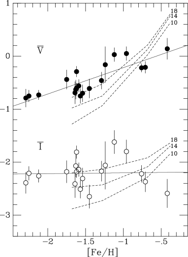
Figure 7: Comparison of the $\overline{M}_{V}$ and $\overline{M}_{I}$ measurements for Galactic globular clusters by Ajhar & Tonry (1994) with the new model (Vazdekis 2000; Salpeter IMF) predictions (dashed lines). The models are for ages of 10.0, 14.1, and 17.8 Gyr (labelled), with the younger ages giving brighter SBF magnitudes. The [Fe/H] values for the globulars are taken from the Harris (1996) electronic catalogue, version dated 22 June 1999, and we have adopted the horizontal branch calibration used in that catalogue to set the distances. The solid lines are simple linear fits to the data.

The globular cluster distances were calculated from the ‘compromise’ relation between the horizontal branch magnitude and metallicity advocated in the current (June 1999) version of the Harris (1996) electronic catalogue:

$$M_{V}({\rm HB})\,=\,0.15\hbox{[Fe/H]}+0.80\,.$$ (4)

The slope here is the same as used in the analysis by Ajhar & Tonry, who adopted the calibration of Carney, Storm, & Jones (1992) based on statistical parallax and Baade-Wesselink measurements of field RR Lyrae stars, but the zero point is brighter by 0.21 mag. However, this zero point is 0.1–0.2 mag fainter than those favoured by recent analyses of Hipparcos subdwarf parallaxes (Gratton et al. 1997; Carretta, et al. 2000), but it accords well with the calibration derived when the RR Lyrae luminosity is set by requiring consistency with the Cepheid distance to the Large Magellanic Cloud (e.g. Walker 1992). Carretta et al. (2000) make note of this last point and so adjust their final calibration fainter by 0.1 mag, concluding that the distances derived from the subdwarf fitting are about $1\sigma$ too large.

All of the above methods for deriving the HB/RR Lyra calibration, as well as HB measurements in M31 globulars (Ajhar et al. 1996; Fusi Pecci et al. 1996), agree fairly well on a slope of 0.15$\pm$0.05, but values of 0.30 or more have also been proposed (e.g., Sandage 1993). Using a distance calibration with a steeper slope makes the derived slope of $\overline{M}$ vs [Fe/H] steeper, and thus more similar to the model predictions. However, as there are more direct and less model-dependent means for deriving the slope of the RR Lyra calibration, we do not allow ourselves this added freedom.

With the distance calibration from Eq. (4), the Ajhar & Tonry (1994) globular cluster data give

$$\overline{M}_{V} = -0.46\;+\;0.44\,(\hbox{[Fe/H]}+1.5)$$

$$\overline{M}_{I} = -2.21\,,$$ (5)

with rms scatters of 0.16 and 0.26 mag in $V$ and $I$, respectively. There is no significant slope in the $I$ band. The models agree well with the $I$-band data in zero point and are marginally too bright (given the $\sim\,$0.2 mag uncertainty in the observational zero point) in the $V$ band, where the metal-poor globulars would require greater model ages. Both data and models exhibit a much steeper dependence for $\overline{M}_{V}$ on metallicity. The models predict an increasingly shallow slope at increasingly lower metallicities in both bands.

We find the agreement between the globular cluster SBF data and the new models encouraging. The agreement is further improved if the more metal-rich globulars are also younger, or, stated another way, this is what the present comparison predicts. The baseline of this comparison needs to be increased with more SBF measurements of higher metallicity globulars (unfortunately these are generally at large distances and low Galactic latitudes, with severe extinction and disk/bulge star contamination), as well as by extending the model predictions to lower metallicities.

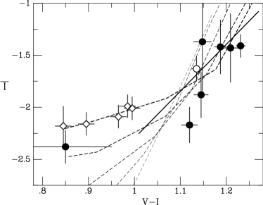
Figure 8: Comparison of $\overline{M}_{I}$ model predictions with measurements for galaxies with Cepheid distances (data from SBF-III). Filled circles are for spirals with bulge $\overline{m}_{I}$ measurements and for the dwarf irregular NGC 5253, which has $(V{-}I){\,=\,}0.85$. Open symbols are for the compact elliptical M32 (circle) and various locations (10–130 arcsec) in the dwarf elliptical NGC 205 (diamonds), both assumed to be at the same Cepheid distance as M31. (The M32 data point represents a mean within a radius of about 2.5 arcmin.) The dashed lines connect models of different metallicity but fixed age; the ages represented are 4.0, 7.1, 10.0, 14.1, and 17.8 Gyr, with heavier lines used for greater ages. The solid line shows the empirically calibrated relation based on SBF measurements to ellipticals in groups with Cepheids distances.

4.2 SBF in Galaxies with Cepheid Distances

Because the method works best for ellipticals, SBF distances are difficult to calibrate against Cepheids. We are forced to attempting the analysis in irregulars and spiral bulges or else associating early- and late-type galaxies via uncertain group membership. Both options are fraught with systematic problems (see Appendix B of SBF-II) but are currently the only means for comparing our models against the Cepheid distance scale. Figure 8 shows the comparison for the $I$ band, the only band with direct SBF measurements in Cepheid-bearing galaxies other than M31. Two of the galaxies in Figure 8 have $\overline{M}_{I}$ values too bright by more than 1$\,\sigma$ as compared to the models. Otherwise the agreement appears reasonably good.

The flattening of the $\overline{M}_{I}$-$(V{-}I)$ relation for galaxies with $(V{-}I)<1.0$ was noted as a puzzle by SBF-I, and these galaxies were excluded from the calibration, but our new SSP models predict this effect. The apparent 18-Gyr age for NGC 205 is surely too high, but this may be misleading due to composite population effects. The combination of old very metal-poor stars with a young high-metallicity component could yield observed position for NGC 205 in Figure 8. In addition, the true distance of this galaxy may well be greater than the assumed M31 Cepheid distance. Observations of both RR Lyra stars (Saha, Hoessel, & Krist 1992) and post-AGB stars (Fullton & Bond 1997) indicate that NGC 205 is about 0.3 mag more distant than M31; if so, its inferred age would decrease by 5 Gyr.

M32 is the only ‘typical SBF galaxy’ in Figure 8, and it appears consistent with the models if placed at the same distance as M31. However, recent spectroscopic population synthesis studies of this galaxy find best-fitting models with solar metallicity, or slightly below, and an age typically 4–6 Gyr (Jones & Worthey 1995; Vazdekis & Arimoto 1999; del Burgo et al. 2000; Trager et al. 2000a). Our models with this age and metallicity (see Table 2) match the observed $(V{-}I)=1.13$ colour of this galaxy but give $\overline{M}_{I}$ too faint by 0.1–0.2 mag. Of course, the spectroscopic analyses used much smaller apertures than the SBF analysis. Rose et al. (2000, in preparation) find that M32 has a radial age/metallicity gradient, even though the optical colours stay nearly constant; thus, a direct comparison to the spectroscopic measurements is not possible.

Despite the potential problems, the group-based empirical relation shown in the figure has encouraging overlap with the models. Section 5 returns in greater detail to the issues of composite populations and differences between the empirical and model SBF calibrations in various bandpasses.

4.3 Fluctuation Colour versus Integrated Colour

Fluctuation colours are different from integrated colours. For instance, Figure 9 plots $(\overline{V}{-}\overline{I})$ against $(V{-}I)$ for globular clusters (Ajhar & Tonry 1994), galaxies (Tonry et al. 1990; this work; SBF-IV), and our new models. Although there is an overall correlation between $(\overline{V}{-}\overline{I})$ and $(V{-}I)$, these quantities have opposite age dependences in our models. As age increases at a fixed metallicity, the model $(\overline{V}{-}\overline{I})$ colour gets bluer while $(V{-}I)$ gets redder. This is a fairly common feature of fluctuation colours in our models. For instance, even though $(V{-}K)$ is nearly independent of age at lower metallicities, $(\overline{V}{-}\overline{K})$ gets nearly a magnitude bluer as age is increased from 5 to 17 Gyr.

Figure 9: The $(\overline{V}{-}\overline{I})$ fluctuation colour is plotted against integrated $(V{-}I)$ for the new models with ages $\geq 4.0\,$Gyr (symbols coded as in Figure 2), the Ajhar & Tonry (1994) globular clusters (filled circles), and the data available for 21 galaxies in the Local Group, Leo, Virgo, and Fornax (filled squares). The models here use a Salpeter ($\mu=1.3$) IMF. The globular cluster NGC 6624 (marked) with $\hbox{[Fe/H]}=-0.4$ has the highest metallicity in the Ajhar & Tonry sample. The arrow shows the effect of increasing the extinction estimate by 0.03 mag.

Figure 10: Same as Figure 9, but for a steeper IMF of unimodal logarithmic slope $\mu=2.3$; the model points have moved significantly redder in $(V{-}I)$ and slightly bluer in $(\overline{V}{-}\overline{I})$, mimicking the effects of age. Although the steep IMF makes the match between models and data better here, other problems arise as a consequence (see text).

The galaxies in Figure 9 lie close to the higher metallicity models, where it becomes more difficult to separate age and metallicity effects. A careful study of radial population gradients within individual ellipticals using this diagram would be interesting. Gradients in single-band fluctuation magnitudes are well known (Tonry 1991; Sodemann & Thomsen 1995, 1996), and simply follow the integrated colour gradients, which tend to be small for giant ellipticals. A significant gradient in the $(\overline{V}{-}\overline{I})$ fluctuation colour would be much more difficult to detect because of the small intrinsic spread and the large uncertainties. However, it might reveal whether the radial population gradient is simply a metallicity gradient or if age gradients are important as well. With the expected high-resolution, wide-field imaging capability of future Hubble Space Telescope (HST) instruments, this kind of study should soon be more feasible.

The globular cluster data in Figure 9 mainly lie among the $\hbox{[Fe/H]}\leq-0.4$, $\hbox{age}\mathrel{\hbox to0.0pt{\lower 3.0pt\hbox{$\mathchar 536\relax$}\hss}\raise 2.0pt\hbox{$\mathchar 318\relax$}}10$ Gyr models, but with an apparently significant age spread. For instance, near $(V{-}I)=0.9$ the data show a significant range in $(\overline{V}{-}\overline{I})$, and although zero-point problems are likely, the trend of the models clearly suggests age variations. We note that the globular cluster NGC 6624, which had the highest metallicity in the Ajhar & Tonry sample, falls in a region of the diagram consistent with its photometrically estimated metallicity of $\hbox{[Fe/H]}=-0.42$. This value is higher than the spectroscopic determinations by 0.3 dex (Vazdekis 1999) to as much as 0.7 dex (Origlia et al. 1997). Although the methods for determining metallicity give discrepant results for this globular, it seems reasonable that SBF measurements would be most consistent with the photometric value.

Figure 9 also reveals a possible shortcoming of the models: they do not get blue enough in $(\overline{V}{-}\overline{I})$ to match several of the $(V{-}I)>0.9$ globulars (this was also apparent in Figure 7). On the other hand, this discrepancy could arise from underestimating the extinction towards these globulars, as illustrated by the reddening vector in the figure. Presumably the models would reach these data points for ages $\mathrel{\hbox to0.0pt{\lower 3.0pt\hbox{$\mathchar 536\relax$}\hss}\raise 2.0pt\hbox{$\mathchar 318\relax$}}20\,$Gyr, but this is unrealistically large. The problem is reminiscent of the difficulty encountered in trying to match the H$\gamma$ absorption indices of globulars (Vazdekis & Arimoto 1999; Gibson et al. 1999).

Figure 10 shows that the symptoms of this problem can be removed with a steeper (unimodal) IMF of slope $\mu=2.3$, which for this plot has effects similar to increasing the age. (The Miller-Scalo-like bimodal IMF of high-mass slope 2.3 basically reproduces the Salpeter IMF results in Figure 9). However, such a steep IMF is inconsistent with observations of the stellar mass function in globulars (Paresce & De Marchi 2000), and makes $(V{-}I)$ too red at a given metallicity. It also implies ages $\mathrel{\hbox to0.0pt{\lower 3.0pt\hbox{$\mathchar 536\relax$}\hss}\raise 2.0pt\hbox{$\mathchar 316\relax$}}7\,$Gyr for some of the globulars, which is inconsistent with ages based on the colour-magnitude diagram. Thus, we continue to prefer the models based on the Salpeter IMF, although they appear to overestimate the ages somewhat.

4.4 Fluctuation Colours and Composite Populations

Blakeslee et al. (1999a) showed a comparison of the observed $(\overline{V}{-}\overline{I})$ vs $(\overline{I}{-}\overline{K})$ for 10 galaxies with the SSP model predictions from Worthey (1993a, 1994). The models had very little overlap with the data, but rather looped around them, approaching only the M32 data point. Thus, the only way to reproduce the data was by combining the SSP models and then specifically picking out the composite populations which overlay the data. Figure 11 updates this comparison using the present set of models, revising the extinction estimates as in SBF-II, and including the $\overline{V}$ data presented in §2. The locus of the Worthey models, as in Blakeslee et al. (1999a), is shown for comparison.

Figure 11: The $(\overline{I}{-}\overline{K})$ fluctuation colour is plotted against $(\overline{V}{-}\overline{I})$ for the new models (symbols as in Figure 2) and data for 12 ellipticals and the bulge of M31. The $V$ data are from Tonry et al. (1990) and the present work; the $I$ data are from SBF-III; the $K$ data are from Luppino & Tonry (1993) (two galaxies), Jensen et al. (1998) (ten galaxies), and Pahre & Mould (1994) (one galaxy). The locus of the single-burst old stellar population models of Worthey (1994) is indicated by a dashed line.

The new models provide a more natural explanation of why the mean $(\overline{V}{-}\overline{I})$ for the galaxies is $\sim\,$2.4 with a relatively small dispersion. As the model metallicity increases, the $(\overline{V}{-}\overline{I})$ colour gets redder (though bluer as the age increases at fixed [Fe/H]), until the metallicity approaches roughly half solar and higher, where $(\overline{V}{-}\overline{I})$ remains near 2.4. The models plotted in Figure 11 use a Salpeter IMF ($\mu=1.3$), but the form of this plot is not very sensitive to the IMF. At the metallicities appropriate to elliptical galaxies, $(\overline{V}{-}\overline{I})$ gets bluer by about 0.08 mag, and $(\overline{I}{-}\overline{K})$ changes by only about 0.03 mag, when the slope of the unimodal IMF is increased to $\mu=2.3$. As before, a bimodal IMF with $\mu\approx 2$ gives results similar to Salpeter.

This figure is, however, very sensitive to the underlying isochrones used in the modeling. As discussed more in the following sections, the gross differences between the present model predictions and those of Worthey are mainly due to the different sets of isochrones used. Liu et al. (2000) also find that their models, which use the stellar tracks of Bertelli et al. (1994), are much closer to the data in this diagram than the Worthey models are. For our models, the discrepancy with the Worthey predictions becomes greater when the Bertelli et al. (1994) isochrones are used: the model points in Figure 11 would be shifted even further to the left and would exhibit considerably more scatter.

Although our new models help us to understand the observed galaxy fluctuation colours better, composite population modeling still appears necessary for the galaxies in Figure 11 with $(\overline{V}{-}\overline{I})\mathrel{\hbox to0.0pt{\lower 3.0pt\hbox{$\mathchar 536\relax$}\hss}\raise 2.0pt\hbox{$\mathchar 316\relax$}}2.3$. We take up this problem in the following section.

5 Theoretical Distance Calibrations

One motivation for this work was to derive the best possible theoretical calibration of the SBF distance method, particularly in the $I$ and near-IR bands. One complication is that our new SSP models do not generally define simple linear relations between $\overline{M}$ and colour. This alone does not indicate disagreement with observations, as actual galaxies are not expected to be homogeneous simple stellar populations. However, it becomes necessary to combine the models in such a way as to reproduce the observed distribution of integrated and fluctuation colours (distance-independent quantities) before fitting for a distance calibration.

5.1 Recipe for the Composite Populations

We wish to combine the homogeneous SSP models into composite systems in such a way as to mimic, at least crudely, the evolution of an elliptical galaxy. We first group the SSP models into three bins according to metallicity: (1) metal-poor, (2) intermediate, and (3) metal-rich, with each bin containing two of the six SSP model metallicities. We then randomly choose one SSP model from each bin, or ‘metallicity component,’ subject to the following age restrictions:

$$14.1\hbox{ Gyr} \leq\;\;\hbox{age(1)}\;\;\leq$$ 17.8 Gyr

$$8.9\hbox{ Gyr} \leq\;\;\hbox{age(2)}\;\;\leq$$ 17.8 Gyr (6)

$$4.0\hbox{ Gyr} \leq\;\;\hbox{age(3)}\;\;\leq \hbox{17.8 Gyr}\,.$$

We use all 14 isochrone ages of 4 Gyr or more calculated by Girardi et al. (2000). This includes all the ages listed in Table 2 plus ages of 4.5, 5.6, 7.1, and 8.9 Gyr.

The three components are then combined with weights $f_{1},f_{2},f_{3}$, which are random numbers normalized so that the composite models have in the mean contributions of 10% from the low-metallicity bin, 40% from the intermediate bin, and 50% from the high-metallicity bin. We experimented with other weightings, but kept these for reasons given in the following sections. The fluctuation luminosity for the composite population is calculated as

$$\overline{L}={{f_{1}{\cdot\,}\langle{L_{1}^{2}}\rangle+f_{2}{\cdot\,}\langle{L_{2}^{2}}\rangle+f_{3}{\cdot\,}\langle{L_{3}^{2}}\rangle}\over{f_{1}{\cdot\,}\langle L_{1}\rangle+f_{2}{\cdot\,}\langle L_{2}\rangle+f_{3}{\cdot\,}\langle L_{3}\rangle}}\;,$$ (7)

where by definition $\langle{L_{i}^{2}}\rangle=\langle L_{i}\rangle{\,\cdot\,}\overline{L}{{}_{i}}$.

We considered incorporating the additional requirement age(1) $\geq$ age(2) $\geq$ age(3), as would necessarily result from pure self-enrichment models. Lifting this restriction in favour of Eqs. (6) is meant to allow for the possibility of merging/accretion or late infall of metal-poor gas. This extra freedom in the ages increases the scatter in the $\overline{M}$-$(V{-}I)$ relations of the following section by $\sim\,$10% and affects the slopes at the $\sim\,$10% level, but does not significantly affect the zero points at our fiducial $(V{-}I)=1.15$ colour.

Finally, we select out the composite models having the same (within 3$\,\sigma$) fluctuation colours as the galaxy data. In practice this includes all composite models with $(\overline{I}{-}\overline{K})>3.65$ and $(\overline{V}{-}\overline{I})>1.95$. About 42% of the models meet these selection criteria. Overall, the mean ages for the metal-poor, intermediate, and metal-rich components are 15.9, 13.0, and 9.3 Gyr, respectively; after culling according to the fluctuation colours, the mean ages become 16.1, 12.9, and 7.6 Gyr, respectively. Among the models in this ‘culled sample,’ 12.9% have the intermediate metallicity component older than the metal-poor component, 11.6% have the metal-rich component older than the intermediate component, and only 2.8% have the metal-rich component older than the metal-poor one. These ‘age-overlap’ percentages are decreased from 14%, 22%, and 7%, respectively, in the pre-selection sample.

The fluctuation-colour selection therefore drives the metal-rich component towards younger ages and significantly decreases the fraction of composite models with ‘age inversion’ (more metal-poor stars being younger than richer ones). It may be tempting to conclude, speculatively, that this result favours self-enrichment models and that the accretion of low-metallicity gas-rich material (and subsequent formation of young, metal-poor stars) is not an important factor in the luminosity grown of ellipticals. This is similar to the conclusions of Trager et al. (2000b). However, our composite population scheme is fairly ad hoc and the model/data comparison uses only two observables (two fluctuation colours). While the results are intriguing, firm conclusions on the evolution of early-type galaxies await more exhaustive analyses with larger data sets.

5.2 Optical SBF Distances

Figure 12 plots the composite model SBF magnitudes in the $VRI$ bands against integrated $(V{-}I)$ colour. The panels on the left show models prior to any selection criteria, while the ones on right have been culled according to their fluctuation colours, as described above. The least-squares fits to the culled models and the rms scatters in the fits are given by

$$\overline{M}_{V} =\;\;+0.74\,+\,4.8\,[(V{-}I)-1.15]\,, \pm\,0.15\,\hbox{mag}\,,$$ (8)

$$\overline{M}_{R} =\;\;-0.21\,+\,4.9\,[(V{-}I)-1.15]\,, \pm\,0.13\,\hbox{mag}\,,$$ (9)

$$\overline{M}_{I} =\;\;-1.47\,+\,4.5\,[(V{-}I)-1.15]\,, \pm\,0.10\,\hbox{mag}\,.$$ (10)

The selection by fluctuation colours has decreased the rms scatters by 28%, 25%, and 22% in $V$, $R$, and $I$, respectively. The statistical uncertainties in the slopes of these relations are $\mathrel{\hbox to0.0pt{\lower 3.0pt\hbox{$\mathchar 536\relax$}\hss}\raise 2.0pt\hbox{$\mathchar 316\relax$}}\,$0.5%, but experimenting with other reasonable metallicity weightings and age restrictions shows that variations of $\pm\,$12% are typical and give a more realistic impression of the uncertainty. The zero points, however, are much more secure, typically varying by $\pm$0.02 mag or less (for a Salpeter IMF; changing the IMF slope can cause variations 4 times greater).

One motivation for the adopted composite population scheme is that it reproduces the slope of 4.5 observed in the $I$ band (SBF-I). Thus, we cannot really claim that these models ‘predict’ the observed $I$-band slope. Rather, the slope was more of an observational constraint in the modeling, similar to the $(\overline{V}{-}\overline{I})$ and $(\overline{I}{-}\overline{K})$ fluctuation colours. For instance, decreasing the mean percentage of metal-poor stars from 10% to 5% increases the $I$-band slope by about 8% and decreases the $V$ slope so that the relation is steeper in $I$, contrary to what is observed. Thus, metal-poor stars appear to be a small but important component of early-type galaxies. Part of the reason the model slopes match the observed ones is that the colour distribution of the composite models, $1.05\mathrel{\hbox to0.0pt{\lower 3.0pt\hbox{$\mathchar 536\relax$}\hss}\raise 2.0pt\hbox{$\mathchar 316\relax$}}(V{-}I)\mathrel{\hbox to0.0pt{\lower 3.0pt\hbox{$\mathchar 536\relax$}\hss}\raise 2.0pt\hbox{$\mathchar 316\relax$}}1.25$, is similar to that of the SBF survey galaxies. The $I$ slope is flatter for bluer populations, as discussed in §4.2 above, and becomes steeper at the red end (see §5.5 below).

Figure 12: Optical $VRI$ SBF magnitudes are plotted against $(V{-}I)$ for composite populations. In the left panels, no selection criteria have been applied to the simulated composite populations; in the right panels, only composite models having $(\overline{V}{-}\overline{I})$ and $(\overline{I}{-}\overline{K})$ fluctuation colours in the observed range for elliptical galaxies are shown. In each case, 1200 points are plotted, and the solid lines are least-squares fits to guide the eye. Note the difference in horizontal scale between the left and right panels. The dashed lines represent the empirical relations in the $V$ (top) and $I$ (bottom) bands, from this work and the $I$-band SBF survey, respectively.

The $V$-band calibration of Eq. (8) agrees well with the observed calibration from Eq. (2). The zero points differ by just 0.03 mag. We note, however, that the adopted empirical zero point relies on the group tie between SBF and Cepheids, which is more secure both in a statistical sense and in the sense that the calibrators are typical of the sample galaxies. Had the ‘direct’ tie, based on fairly uncertain SBF measurements in spiral bulges, been adopted in §2.2, the empirical zero point ($\overline{M}_{V}^{0}=+0.65$) would 0.09 mag brighter than the zero point of Eq. (8).

The empirical $I$ zero point $\overline{M}_{I}^{0}=-1.62$ adopted in §2.2 is 0.15 mag brighter than the Eq. (10) calibration. A similar offset was found in §4.2 when comparing $\overline{M}_{I}$ for M32 to the SSP models. Had we adopted the ‘direct’ Cepheid tie from SBF-II, the discrepancy would be 0.27 mag. We take this as additional evidence in favour of the group calibration. Further, we note that the dynamical distance to the NGC 4258 water maser (Herrnstein et al. 1999) indicates that the Cepheid distance scale may be too long by 0.2 mag (Maoz et al. 1999). If so, we would achieve excellent agreement between the group $I$-band SBF calibration and our theoretical calibration. The theoretical $V$-band calibration would then be $\sim 0.2\,$mag too bright, i.e., the $(\overline{V}{-}\overline{I})$ colours of our composite models are too blue by about 0.15 mag. It is possible to ‘fix’ this situation by weighting them heavily towards the high metallicity component, but then the $(V{-}I)$ colours become redder than the SBF survey galaxies by $\sim\,$0.08 mag and the $I$ slope increases to $\sim 6$.

Finally, we note that our theoretical $\overline{M}_{I}$ calibration is $\sim\,$0.35 mag fainter than the calibration from the Worthey (1994) models (see SBF-I; Blakeslee et al. 1999a). At solar metallicity, the $(V{-}I)$ colours of the Worthey models are $\sim\,$0.07 mag redder than ours. These differences are mainly due to the different isochrone sets. As discussed in detail by Charlot et al. (1996), the mean luminosity of the RGB stars is about 25% greater in the isochrones used by Worthey. For the integrated light, this is mostly offset by the greater quantity of stars on the Padua RGB. However, even if these two competing effects completely cancel for the integrated light, the luminosity variance from the Worthey RGB will be 0.25 mag brighter. G. Worthey’s stellar population page on the World Wide Web provides the option of replacing his original isochrones with the Bertelli et al. (1994) isochrones. Using this option makes the Worthey models at solar metallicity bluer in $(V{-}I)$ by nearly 0.1 mag and fainter in $\overline{M}_{I}$ by $\sim\,$0.50 mag; the resulting calibration is about 0.2 mag fainter than our $\overline{M}_{I}$ calibration (which uses the more recent Padua isochrones and a completely different set of transformations). Yet, the new Liu et al. (2000) models use the Bertelli et al. tracks and obtain a zero point similar to the original Worthey (1994) one. Table 3 provides a summary scorecard of the various empirical and theoretical $I$ SBF calibrations.

This discussion illustrates how the combination of integrated colours and SBF magnitudes can provide important new constraints for stellar evolution. At the same time, the sensitivity of SBF to the finer details of RGB evolution means that any theoretical calibration will at this point be inherently uncertain.

Table 3: Comparison of $I$-band SBF Zero Points

$\overline{M}^{0}_{I}\,$	Method	Source
$-$1.74	spiral	SBF-II
$-$1.79	spiral	Ferrarese et al. (2000)
$-$1.54	spiral	SBF-II, adjusted for NGC 4258
$-$1.62	group	SBF-II
$-$1.42	group	SBF-II, adjusted for NGC 4258d
$-$1.47	theory	This work, Eq. 10
$-$1.81	theory	SBF-I, Worthey (1994) models
$-$1.25	theory	Worthey Web page, Padua option
$-$1.79	theory	Liu et al. (2000)

Figure 13: Model $I$-band SBF magnitude $\overline{M}_{I}$ and $(V{-}I)$ colours are plotted against Mg₂ for our composite models. As in Figure 12, the left panels show models without any selection criteria, and the right panels show models selected based on fluctuation colours, with the solid lines being least-squares fits. Note the difference in horizontal scale between the left and right panels. The dashed line in the top panels represents the empirical relation from Thomsen et al. (1997). The dashed line in the lower panels shows the relation between $(V{-}I)$ and Mg₂ obtained by tying together the two separate $\overline{M}_{I}$ calibrations; for visibility, this line is extended well beyond its true validity limits. Data for nearly 200 galaxies (open diamonds) in common between the SBF and SMAC surveys are shown for comparison; their Mg₂ values have been shifted by $-0.04$ as an overall estimate of the correction for aperture differences.

5.3 Mg₂ versus $(V{-}I)$ for the Calibration

The $I$-band SBF distance indicator has also been calibrated against the Mg₂ absorption index (Thomsen et al. 1997). This calibration, using $\overline{m}_{I}$ data from Sodemann & Thomsen (1995) and the Mg₂ measurements of Davies, Sadler, & Peletier (1993), is based solely on the internal gradients in NGC 3379. It is only strictly applicable over the range $0.24<\hbox{Mg}_{2}<0.28$. The top panels of Figure 13 show the corresponding relation for our composite models. The relation in the top right panel is

$$\overline{M}_{I}\;=\;-1.50\,+\,8.6\,[{\rm Mg}_{2}-0.22]\,,\;\;\pm\,0.07\,\hbox{mag}\,.$$ (11)

The slope agrees well with the Thomsen et al. calibration, but the zero point is again 0.15 mag too faint. Although the scatter is small, calibrating the observations is much more difficult. It requires a well-orchestrated combination of imaging and spectroscopy, and absorption measurements are difficult well outside the bright galaxy centre. Also, there is the unresolved (and unmodeled) issue over whether the colours, and SBF magnitudes for that matter, should follow the Fe abundance or the Mg overabundance.

The consistency between the Mg₂ and $(V{-}I)$ calibrations is illustrated in the lower panels of Figure 13. We can tie these two quantities together via their respective $\overline{M}_{I}$ calibrations, which for $(V{-}I)$ is based on $\sim\,$150 galaxies and for Mg₂ is based on one galaxy. The resulting ‘empirical’ line, extended well beyond the true limits of applicability, almost perfectly overlays the model predictions. However, the agreement may be somewhat coincidental. A shift of only 0.02 mag in the Mg₂ data for NGC 3379 (as, for instance, in the measurements by Vazdekis et al. 1997) would eliminate the offset in the top panel of Fig. 13 and cause an offset in the lower panel. For a further comparison we show in the bottom panel galaxies in common between the SBF and SMAC (Smith et al. 2000; Hudson et al. 2000) surveys. The SMAC Mg₂ values have been shifted by $-0.04$ mag as an approximate allowance for aperture effects. The galaxy points follow a shallower slope than the models, perhaps because of the increasing Mg enhancement for redder, more luminous ellipticals.

Figure 14: Similar to Figure 12 except for the near-IR bandpasses. Again, note the horizontal scale difference between the left and right panels. The dashed line in the bottom panels is the empirical two-parameter group calibration from table 7 of Jensen et al. (1998).

5.4 Near-Infrared SBF Distances

Figure 14 shows the composite model relations between $(V{-}I)$ colour and the near-IR SBF magnitudes. The calibrations derived from the simple least-squares fits are

$$\overline{M}_{J} =\;\;-3.72\,+\,3.0\,[(V{-}I)-1.15]\,, \pm\,0.09\,\hbox{mag}\,,$$ (12)

$$\overline{M}_{H} =\;\;-4.92\,+\,3.0\,[(V{-}I)-1.15]\,, \pm\,0.10\,\hbox{mag}\,,$$ (13)

$$\overline{M}_{K} =\;\;-5.38\,+\,2.9\,[(V{-}I)-1.15]\,, \pm\,0.10\,\hbox{mag}\,.$$ (14)

Again, the slopes show variations at about the 12% level for different (reasonable) composite modeling assumptions, while the zero points remain fixed at the $\pm\,$0.02 mag level. The selection by fluctuation colours decreases the rms scatters about Eqs. (12)-(14) by $\sim\,$70% in each case. Thus, a measurement of the actual scatter in a large and diverse sample of early-type galaxies could provide insight into the variety of the stellar mixtures in these galaxies.

Our model $K$-band zero point at $(V{-}I)=1.15$ is 0.24–0.36 mag fainter than the empirical one (depending on whether the group or direct Cepheid tie is used), which is based on measurements by Jensen et al. (1998). We should note that the $K$-band data are more weighted towards the red than the $I$-band survey data, so a better fiducial colour might be $(V{-}I)=1.2$, in which case the zero point discrepancy is 0.3–0.42 mag. Interestingly, the former Padua isochrones (Bertelli et al. 1994), because of their more infrared luminous AGB, make the model $K$ zero point brighter by 0.5 mag or more, i.e., about 0.2 mag brighter than the empirical zero point. However, the agreement becomes much worse in the $I$ band, with the theoretical zero point being 0.4–0.5 mag too faint because of the cooler RGB. Again, all the same caveats apply as in §5.2 with regard to the sensitivity of these calibrations to stellar evolution. Clearly we will have learned much by the time the models reproduce the SBF data in all bands.

It is noteworthy that the slopes of Eqs. (12)–(14) are positive, i.e., in the same sense as the slopes for optical SBF (although the $K$-band slope is negative before the selection by fluctuation colours). This is in the sense opposite that given by either the Worthey models or the Liu et al. (2000) models, which both predict a brightening of the near-IR SBF magnitudes for redder populations. The dimming of our model near-IR SBF magnitudes in redder populations agrees better with observations (Jensen et al. 2000, in preparation). In particular, we disagree with the conclusion by Liu et al. (2000) that the $K$-band data imply that ellipticals all have roughly solar metallicity but a large spread in age. In the context of our models, the observed trend could well be due to metallicity variations.

Redder than $(V{-}I)=1.2$, Figure 14 shows a flattening of the predicted relations, so that a constant $\overline{M}$ calibration in the near-IR would work best for the reddest ellipticals. Interestingly, just the opposite happens in the $I$-band, as we discuss in the following section.

5.5 SBF with WFPC2

Ajhar et al. (1997) measured SBF magnitudes in the WFPC2 F814W bandpass for 16 early-type galaxies observed with HST. Although F814W is similar to Cousins $I$, the data gave a steeper slope of $6.5\pm 0.8$ for the calibration against $(V{-}I)$. In an effort to understand this, we have computed SBF magnitudes for our models in the WFPC2 filter system using the empirical and synthetic photometric transformations from Holtzman et al. (1995). Unfortunately, the empirical transformations are only determined for stars with $(V{-}I)\mathrel{\hbox to0.0pt{\lower 3.0pt\hbox{$\mathchar 536\relax$}\hss}\raise 2.0pt\hbox{$\mathchar 316\relax$}}1.4$. For redder stars, including higher metallicity RGB stars (the most important ones for us), they derived synthetic transformations using template stellar spectra and model bandpasses. It is this sort of theoretical transformation that we have sought to avoid in using the new Vazdekis models, but here we are forced to it.

Figure 15: A comparison of the synthetic stellar transformations from WFPC2 to Johnson-Cousins bandpasses (Holtzman et al. 1995 – dashed lines) with the SBF transformations ‘measured’ from the SSP models (symbols as in Figure 2). Small but systematic errors will be made in assuming that the stellar transformations will apply to the SBF measurements. The true errors will be larger than implied by this figure, as the Holtzman et al. transformations were built into our code for computing the WFPC2 magnitudes of the constituent model stars, but actual stars will deviate from these transformations. Because we were forced to rely heavily on synthetic transformations (shifted in a fairly arbitrary way into agreement with the empirical transformations), our model SBF magnitudes for the WFPC2 filters are more uncertain than for the standard bandpasses.

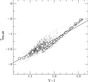
Figure 16: The F814W SBF magnitudes are plotted against $(V{-}I)$ for composite models (after the fluctuation-colour selection). Again, 1200 individual composite models are plotted with a linear fit (solid line), but the open circles represent averages in $(V{-}I)$ steps of 0.02 mag for over 80,000 model realizations. A linear fit to the open circles with $(V{-}I)>1.18$ (short-dashed line) has a slope in close agreement with the slope of the F814W SBF calibration derived by Ajhar et al. (1997) (long-dashed line). The vertical offset between the models and the empirical line is 0.06 mag, or 0.09 mag less than the corresponding offset for Cousins $I$, but this small discrepancy may be due at least in part to systematic errors in the synthetic stellar transformations.

As Holtzman et al. discuss, their empirical and synthetic transformations do not always agree. However, we noticed that the two types of $I$–F814W transformation intersect at $(V{-}I)=1.31$. For consistency, we then shifted the $V$–F555W and $R$–F675W synthetic transformations by $\sim\,$0.023 mag into agreement with the empirical ones at $(V{-}I)=1.31$. We used the empirical transformation for model stars bluer than this and the synthetic one for redder model stars. After transforming all the stars, we calculate the SBF magnitudes. Figure 15 shows the differences between the standard and WFPC2 $V$ and $I$ SBF magnitudes as a function of $(\overline{V}{-}\overline{I})$, and compares these differences to the stellar transformations. Even though these are precisely the transformations used for the model stars in this colour range, there are systematic (though small) differences with the final SBF transformations. This should be no surprise: the spectrum of the fluctuations is quite different from a stellar spectrum, but it is a point often casually overlooked.

Figure 16 shows the resulting relation between $\overline{M}_{{\rm 814W}}$ and $(V{-}I)$ for the culled sample of composite models. It has the same overall 4.5 slope as in the standard $I$ band, and is shifted fainter by 0.06 mag (but this result depends on the uncertain synthetic transforms). However, there is a steepening of the relation starting around $(V{-}I)=1.2$. To illustrate, we compute the running average of $\overline{M}_{{\rm 814W}}$ in $(V{-}I)$ steps of 0.02 and plot the results in the figure. The Ajhar et al. (1997) calibrating galaxies are distributed from $(V{-}I)=1.15$ to $(V{-}I)=1.31$, with 75% being redder than 1.20. This is because the WFPC2 images show only the red galaxy centres. The slope of the running averages at $(V{-}I)>1.18$ is 6.2 [and changes by $\pm 0.3$ as the starting $(V{-}I)$ is changed by $\pm 0.02$], in good agreement with the Ajhar et al. result. Thus, these new models for the first time resolve the puzzle of the steeper F814W slope: it boils down to a slightly nonlinear relation coupled with differences in sample selection.

6 The Fluctuation Star Count

Recently, SBF-IV introduced the parameter $\overline{N}$ as the ratio, expressed in magnitudes, of the total apparent flux from a galaxy to the flux in the fluctuation signal. This ratio is independent of distance, photometric calibration, and extinction; it corresponds to the total luminosity of a galaxy in units of a typical giant star within that galaxy:

$$\overline{N}\,=\,\overline{m}-m_{\rm tot}\,=\,+2.5\,\log\left[L_{\rm tot}\over\overline{L}\right]\,,$$ (15)

where $m_{\rm tot}$ is the total apparent magnitude and $L_{\rm tot}$ the total luminosity. Put another way, if all stars in a galaxy were of magnitude $\overline{m}$, then $\overline{N}$ would be 2.5 times the logarithm of the total number of stars. SBF-IV therefore called $\overline{N}$ the “fluctuation star count,” but it is known to the authors for convenience as the “Tonry number.”

SBF-IV showed that $\overline{N}$ can be used as an alternative calibration in measuring SBF distances. The calibration they derived, adjusted to our group-based zero point (§2.2), is

$$\overline{M}_{I}=-1.62+0.14(\overline{N}-20)\,.$$ (16)

Although this introduces covariance between $\overline{m}_{I}$ and $\overline{M}_{I}$, the final distance modulus is actually 14% less sensitive to errors in $\overline{m}_{I}$. Moreover, the necessity of measuring $(V{-}I)$ to an accuracy of 0.022 mag in order to limit the distance error from photometry to $\mathrel{\hbox to0.0pt{\lower 3.0pt\hbox{$\mathchar 536\relax$}\hss}\raise 2.0pt\hbox{$\mathchar 316\relax$}}0.1\,$mag is replaced by the much less stringent requirement of measuring $m_{\rm tot}$ to an accuracy of 0.7 mag. Similarly, the sensitivity to errors in the Galactic extinction is cut nearly in half for the $\overline{N}$ calibration.

However, SBF-IV cautioned against dropping $(V{-}I)$ altogether in favour of $\overline{N}$. The $(V{-}I)$ calibration is based purely on stellar population properties, whereas the $\overline{N}$ calibration essentially relies on the fundamental plane (FP) of elliptical galaxies and may be subject to systematic effects, such as environmental influences or the presence of a disk component. SBF-IV showed that $\overline{N}$ has a tight correlation with stellar velocity dispersion for SBF survey ellipticals:

$$\log(\sigma)=2.22+0.10\,(\overline{N}-20)\,,$$ (17)

where $\sigma$ is in km s^-1, and the scatter is 0.070 dex. The connection with the FP becomes transparent if we invert this relation to get

$$L_{\rm tot}\;=\;10^{8}\overline{L}\,\left(\sigma\over 165{\,\rm km\,s^{-1}}\right)^{4.0}.$$ (18)

Eq. (18) superficially resembles the classical Faber-Jackson relation (Faber & Jackson 1976), but it contains an implicit correction for the mass-to-light ratio via the $\overline{L}$ term, with its strong stellar-population dependence. This explains why the scatter is similar to that of the inverse FP (e.g., Hudson et al. 1997), and less than half that of Faber-Jackson.

In order to model the behaviour of $\overline{N}$, we must assume some relation between the galaxy luminosity, or mass, and the stellar population. Perhaps the most common form this takes is the Mg₂-$\sigma$ relation (Dressler et al. 1987), conventionally interpreted as a pure mass–metallicity relation (e.g., Bender, Burstein, & Faber 1993; Guzmán, Lucey, & Bower 1993; but see also Trager et al. 2000b). However, we wish to avoid the use of Mg₂ here because it explicitly brings in the alpha-enhancement issue.

Instead, we simply derive the following relation between the $(V{-}I)$ colours of the SBF survey galaxies (SBF-IV) and the velocity dispersions of these galaxies from the homogenized SMAC sample (Hudson et al. 2000):

$$(V{-}I)\,=\,0.71+0.20\log(\sigma)\,.$$ (19)

Details of the comparison of the SBF and FP parameters will be given by Blakeslee et al. (2000, in preparation). Next we assume that the dynamical mass of a galaxy is given by $M=5\sigma^{2}r_{e}/G$ (e.g., Bender et al. 1992; Jørgensen 1999) and make the zeroth-order assumption that all ellipticals have effective radii $r_{e}=6$ kpc. Finally, we assume that the initial stellar mass is half the dynamical mass and then use the model mass-to-light ratios to derive $L_{\rm tot}$ and $\overline{N}$.

Figure 17 illustrates that our crude set of assumptions produces an $\overline{M}_{I}$-$\overline{N}$ relation very similar to the observed one. The slope of the composite model relation is 0.18, while the empirical slope is $0.14\pm 0.04$, and the scatter is 0.095 mag (the slope and scatter would change to 0.20 and 0.074 mag, respectively, if we culled as in the previous section). The zero points of the model and empirical relations are also similar in Figure 17, but this of course depends on the values assumed for $r_{e}$ and the fraction of the mass in stellar material. We have provided only a fairly schematic explanation, based on scaling laws, of why the $\overline{N}$ distance calibration works. A true theoretical calibration of this method must come from further developments in the semi-analytic modeling of early-type galaxy formation (e.g., Cole et al. 1994; Baugh, Cole, & Frenk 1996; Kauffmann & Charlot 1998).

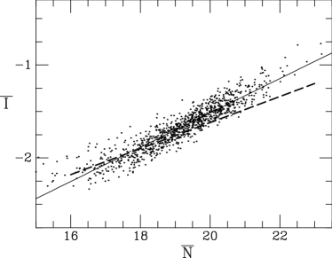
Figure 17: $\overline{M}_{I}$ for the composite models is plotted against the Tonry fluctuation number $\overline{N}$, which has been computed assuming an empirical colour–velocity dispersion relation. The solid line is a least-squares fit to the models, and the thick dashed line is the empirical relation from SBF-IV (Tonry et al. 2000b).

7 Summary and Conclusions

We have presented new $V$-band SBF measurements for five early-type galaxies in the Fornax cluster. Along with Virgo and Leo $\overline{V}$ data from Tonry et al. (1990), these have been used to derive an empirical, Cepheid-calibrated $\overline{M}_{V}$-$(V{-}I)$ distance indicator. The slope of this relation is $5.3\pm 0.8$, similar to the $\overline{M}_{I}$-$(V{-}I)$ empirical slope of 4.5 (SBF-I). We find a mean fluctuation colour $(\overline{V}{-}\overline{I})=2.4$ for our fairly homogeneous set of ellipticals, with a dispersion of only 0.15 mag, comparable to the measurement error.

New stellar population models, updated from those of Vazdekis et al. (1996) with the isochrones of Girardi et al. (2000) and a new set of empirical transformations, have been employed to calculate SBF magnitudes and integrated colours for six different metallicities and a wide range of ages. The age-metallicity degeneracy in the optical $\overline{M}$-colour relations is less for these models than for the models of Worthey (1994), although there is still a high degree of degeneracy in the relation against Mg₂ at intermediate and high metallicities. In the near-IR bands, the model SBF magnitudes have much shallower dependences on colour/metallicity. Below solar metallicity, they depend solely on age, while the integrated colour depends almost solely on metallicity. Thus, the $\overline{M}_{H}$ vs. $(I{-}K)$ plot completely breaks the age-metallicity degeneracy for the lower metallicity models. This could be an important new avenue in stellar population studies.

We have examined the sensitivity of our SBF predictions to changes in the isochrones, theoretical-to-observational transformations, and the IMF. We find that using the former set of Padua isochrones makes the SBF magnitudes 0.1–0.2 mag fainter in the optical and about 0.5 mag brighter in the near-IR. Using theoretical transformations instead of our empirical ones can change the $\overline{M}_{I}$ predictions by nearly 0.5 mag and $\overline{M}_{H}$ by up to 0.7 mag; the changes for the other bands are at the 0.1–0.2 mag level. Thus, the isochrones and the transformations have about equal importance for the SBF results. On the other hand, different IMFs yield fairly similar $\overline{M}$-colour relations in the optical because the IMF effects are largely degenerate with age and metallicity, as noted by Worthey (1993a). This is less true in the near-IR, where the steeper IMF still makes the model colour redder (like metallicity) and $\overline{M}$ fainter (like age), but age and metallicity are no longer degenerate.

The $\overline{M}_{V}$ and $\overline{M}_{I}$ magnitudes of our low metallicity models have been tested against observations for 19 globular clusters. The models agree fairly well, especially if younger ages are taken at higher metallicities, with the data in both zero point and metallicity dependence, which is very weak in the $I$-band. Model calculations at lower metallicities and SBF measurements of higher metallicity globulars (if possible) would allow for much better tests. At any single metallicity, the models predict an anticorrelation between $(\overline{V}{-}\overline{I})$ fluctuation colour and integrated $(V{-}I)$ colour: increasing the age makes $(\overline{V}{-}\overline{I})$ bluer and $(V{-}I)$ redder, although they both become redder with increasing metallicity. The models further imply that the observed spread in $(\overline{V}{-}\overline{I})$ at a fixed $(V{-}I)$ should be interpreted as a spread in age among the globulars. However, some of the globulars are too blue in $(\overline{V}{-}\overline{I})$ (and thus too old) to be match models. This could in part be due to errors in the extinction estimates. At high metallicities, the models predict $(\overline{V}{-}\overline{I})\approx 2.4$, in good agreement with the observations of elliptical galaxies.

Because the single-metallicity, single-age models do not yield completely monotonic relations between $\overline{M}$ and colour, we adopt a Monte Carlo approach to making composite population models from three metallicity bins with different (fairly loose) restrictions on age. We then select out the models that reproduce the observed (distance-independent) fluctuation colours of early-type galaxies. This procedure reproduces well the $(V{-}I)$ colour range of elliptical galaxies and the empirically well-determined slope of $\overline{M}_{I}$ against $(V{-}I)$. If we reduce the mean number of metal poor stars in the models from 10% to 5%, the $I$-band SBF slope becomes marginally too steep, and steeper than the $V$-band slope, contrary to observations. This is due to the flattening of the $\overline{M}_{I}$-$(V{-}I)$ relation in bluer populations, seen in both the data and our models, and is a palpable indication of the presence of metal-poor stars in early-type galaxies. Similarly, we find that the $I$ slope becomes steeper for redder composite populations, those with few metal-poor stars. This explains the steep slope found by Ajhar et al. (1997) for HST F814W observations of elliptical galaxy centres, which are usually quite red.

Although the slopes of the model $\overline{M}$-$(V{-}I)$ relations are fairly sensitive to the details of the composite model prescription, the zero points at $(V{-}I)=1.15$ are not. The zero point of the model $\overline{M}_{V}$ calibration is only 0.03 mag brighter than the empirically determined zero point from §2. If the ‘direct’ (but observationally more precarious) tie of SBF to the Cepheid distance scale via spiral bulges were adopted instead of the group tie, then the theoretical calibration would be 0.09 mag fainter than the empirical one. The theoretical $\overline{M}_{I}$ zero point is 0.15 mag fainter than the empirical one (or 0.27 mag for the direct tie). On the other hand, if the Cepheid distance scale were revised to match the dynamically measured distance to the water maser in NGC 4258, then the theoretical and empirical $\overline{M}_{I}$ zero points would agree closely (at the expense of the empirically less secure $\overline{M}_{V}$ calibration). Our theoretical $\overline{M}_{I}$ calibration is $\sim\,$0.35 mag fainter than the calibration given by the Worthey models; this difference appears to stem from the different isochrones used in the two sets of models.

The variation of $\overline{M}_{I}$ with Mg₂ for the models is in good accord with that obtained by Thomsen et al. (1997) from the internal gradients of NGC 3379. Again, the theoretical zero point is 0.15 mag fainter than observed. This relation is predicted to have less scatter than the calibration against $(V{-}I)$, but the distances would be much more challenging from an observational point of view, unless the SBF measurements are restricted to the bright galaxy centres, as for example with HST imaging. Also, the models do not include the effects of Mg overabundance on either the linestrength predictions or the isochrone temperatures, and it is unclear how this would affect the theoretical calibration.

Our composite modeling predicts that the slope of the near-IR $\overline{M}$-$(V{-}I)$ relation will have the same sense as in the optical, in contrast to the predictions of the Worthey (1994) models and the Liu et al. (2000) models. Our predicted relation then becomes nearly flat for $(V{-}I)>1.2$, (just the opposite of the behaviour seen in the $I$ band). The slope of our derived relations depends on our procedure for selecting out composite models based on their fluctuation colours. The selection criteria also greatly reduce the scatter in the near-IR $\overline{M}$-$(V{-}I)$ relations. Observational studies of the true slope and scatter, and further investigation into the range of fluctuation colours among elliptical galaxies, would be important from the standpoint of both stellar population and distance studies. The $\overline{M}_{K}$ zero point given by our models is 0.24 mag fainter than the empirically calibrated one (or 0.36 mag fainter with the direct tie). This discrepancy depends strongly on the temperature structure of the isochrones, including the AGB.

Finally, we have used mass-colour scaling relations to investigate the recently-introduced Tonry number $\overline{N}$, which describes the luminosity of a galaxy in units of a typical giant star. The simple scaling relations combined with the stellar population models can reproduce the observed dependence of $\overline{M}_{I}$ on $\overline{N}$ from SBF-IV. However, a true theoretical calibration of this form of the SBF method requires more physically-motivated evolutionary models.

Overall, our model SBF predictions are consistent with observations at the $\sim\,$0.2 mag level in the optical and at the $\sim\,$0.3 mag in the near-IR. The present uncertainties in the empirical calibrations are thought to be about a factor of two smaller than this. These results therefore present challenges for stellar evolution and population synthesis. We have noted that SBF magnitudes are acutely sensitive to the distribution and properties of evolved stars, particularly on the RGB, which in turn are sensitive to fairly ill-constrained things such as the colour-temperature scale for the coolest stars, the helium fraction, the prescription for convection, variations in elemental abundance ratios, diffusion, etc. However, it is precisely this sensitivity that gives SBF its own unique vista, as compared to more traditional observables, and should make multi-band SBF observations an important constraint for future stellar population modeling.

References

- [Ajhar et al. 1996] Ajhar, E. A., et al. 1996, AJ, 111, 1110
- [Ajhar et al. 1997] Ajhar, E. A., Lauer, T. R., Tonry, J. L., Blakeslee, J. P., Dressler, A., Holtzman, J. A., Postman, M. 1997, AJ, 114, 626
- [Ajhar & Tonry 1994] Ajhar, E. A. & Tonry, J.L. 1994, ApJ, 429, 557
- [Alonso Arribas & Martinez-Roger 1996] Alonso, A., Arribas, S. & Martinez-Roger, C. 1996, A&A, 313, 873
- [Alonso Arribas & Martinez-Roger 1999] Alonso, A., Arribas, S. & Martinez-Roger, C. 1999, A&AS, 140, 261
- [Alonso et al. 1997] Alonso, A., Salaris, M., Martinez-Roger, C., Straniero, O. & Arribas, S. 1997, A&A, 323, 374
- [Baugh, Cole and Frenk (1996)] Baugh, C. M., Cole, S., & Frenk, C. S. 1996, MNRAS, 283, 1361
- [Bender, Burstein and Faber (1992)] Bender, R., Burstein, D., & Faber, S. M. 1992, ApJ, 399, 462
- [Bender, Burstein and Faber (1993)] Bender, R., Burstein, D., & Faber, S. M. 1993, ApJ, 411, 153
- [Bertelli Bressan & Chiosi 1985] Bertelli, G., Bressan, A. G. & Chiosi, C. 1985, A&A, 150, 33
- [Bertelli et al. 1994] Bertelli, G., Bressan, A., Chiosi, C., Fagotto, F. & Nasi, E. 1994, A&AS, 106, 275
- [Bessell Wood Brett & Scholz 1991] Bessell, M. S., Wood, P. R., Brett, J. M. & Scholz, M. 1991, A&AS, 89, 335
- [Blakeslee, Ajhar, & Tonry 1999] Blakeslee, J. P., Ajhar, E. A., & Tonry, J. L. 1999a, in Post-Hipparcos Cosmic Candles, eds. A. Heck & F. Caputo (Boston: Kluwer), 181
- [Blakeslee et al. 1999b] Blakeslee, J. P., Davis, M., Tonry, J. L., Dressler, A., & Ajhar, E. A. 1999b, ApJ, 527, L73 (SBF-III)
- [Blakeslee & Tonry 1996] Blakeslee, J. P. & Tonry, J. L. 1996, ApJ, 465, L19
- [Borges Idiart de Freitas Pacheco & Thevenin 1995] Borges, A. C., Idiart, T. P., de Freitas Pacheco, J. A., & Thevenin, F. 1995, AJ, 110, 2408
- [Bruzual & Charlot 1993] Bruzual, G. A. & Charlot, S. 1993, ApJ, 405, 538
- [Bruzual 1983] Bruzual, G. A. 1983, ApJ, 273, 205
- [Buzzoni 1993] Buzzoni, A. 1993, A&A, 275, 433
- [Buzzoni 1995] Buzzoni, A. 1995, ApJS, 98, 69
- [Charlot, Worthey & Bressan 1996] Charlot, S., Worthey, G. & Bressan, A. 1996, ApJ, 457, 625
- [Carney Storm & Jones 1992] Carney, B. W., Storm, J. & Jones, R. V. 1992, ApJ, 386, 663
- [Carretta et al. 2000] Carretta, E., Gratton, R. G., Clementini, & G. Fusi Pecci, F. 2000, ApJ, in press
- [Cohen Blakeslee & Ryzhov 1998] Cohen, J. G., Blakeslee, J. P. & Ryzhov, A. 1998, ApJ, 496, 808
- [Cole et al. (1994)] Cole, S., Aragon-Salamanca, A., Frenk, C. S., Navarro, J. F., & Zepf, S. E. 1994, MNRAS, 271, 781
- [Davies Sadler Peletier 1993] Davies, R. L., Sadler, E. M. Peletier, R. F. 1993, MNRAS, 262, 650
- [del Burgo et al] del Burgo, C., Peletier, R. F., Vazdekis, A., Arribas, S., & Mediavilla, E. 2000, MNRAS, in press
- [Dressler et al. (1987)] Dressler, A., Lynden-Bell, D., Burstein, D., Davies, R. L., Faber, S. M., Terlevich, R. J., & Wegner, G. 1987, ApJ, 313, 42
- [Faber 1972] Faber, S. M. 1972, A&A, 20, 361
- [Faber and Jackson (1976)] Faber, S. M. & Jackson, R. E. 1976, ApJ, 204, 668
- [Ferrarese et al. 2000] Ferrarese, L., et al. 2000, ApJ, 529, 745
- [Fullton and Bond (1997)] Fullton, L. K. & Bond, H. E. 1997, BAAS, 191, 1912
- [Fusi Pecci et al. 1996] Fusi Pecci, F., et al. AJ, 112, 1461
- [Gibson et al. 1999] Gibson, B. K., Madgwick, D. S., Jones, L. A., Da Costa, G. S. & Norris, J. E. 1999, AJ, 118, 1268
- [Girardi and Bertelli (1998)] Girardi, L. & Bertelli, G. 1998, MNRAS, 300, 533
- [Girardi Bressan Bertelli & Chiosi 2000] Girardi, L., Bressan, A., Bertelli, G. & Chiosi, C. 2000, A&AS, 141, 371
- [Gratton et al. 1997] Gratton, R. G., Fusi Pecci, F., Carretta, E., Clementini, G., Corsi, C. E. & Lattanzi, M. 1997, ApJ, 491, 749
- [Grillmair, Forbes, Brodie and Elson (1999)] Grillmair, C. J., Forbes, D. A., Brodie, J. P., & Elson, R. A. W. 1999, AJ, 117, 167
- [Groenewegen and de Jong (1993)] Groenewegen, M. A. T. & de Jong, T. 1993, A&A, 267, 410
- [Gunn & Stryker] Gunn, J. E. & Stryker, L. L. 1983, ApJS, 52, 121
- [Guzman, Lucey and Bower (1993)] Guzman, R., Lucey, J. R., & Bower, R. G. 1993, MNRAS, 265, 731
- [Harris 1996] Harris, W.E. 1996, AJ, 112, 1487
- [Hauschildt et al. 1999] Hauschildt, P. H., Allard, F., Ferguson, J., Baron, E. & Alexander, D. R. 1999, ApJ, 525, 871
- [Herrnstein et al. 1999] Herrnstein, J. R., et al. 1999, Nature, 400, 539
- [Holtzman et al. 1995] Holtzman, J. A., Burrows, C. J., Casertano, S., Hester, J. J., Trauger, J. T., Watson, A. M. & Worthey, G. 1995, PASP, 107, 1065
- [Hudson et al. 2000] Hudson, M. J., Lucey, J. R., Smith, R. J., Schlegel, D. J., & Davies, R. L. 2000, MNRAS, submitted
- [Hudson, Lucey, Smith and Steel (1997)] Hudson, M. J., Lucey, J. R., Smith, R. J., & Steel, J. 1997, MNRAS, 291, 488
- [Jensen et al. 1996] Jensen, J.B., Luppino, G.A., & Tonry, J.L. 1996, ApJ, 468, 519
- [Jensen Tonry & Luppino 1998] Jensen, J. B., Tonry, J. L. & Luppino, G. A. 1998, ApJ, 505, 111
- [Jones & Worthey 1995] Jones, L. A. & Worthey, G. 1995, ApJ, 446, L31
- [Jørgensen (1999)] Jørgensen, I. 1999, MNRAS, 306, 607
- [Kauffmann and Charlot (1998)] Kauffmann, G. & Charlot, S. 1998, MNRAS, 294, 705
- [Kodama & Arimoto 1997] Kodama, T. & Arimoto, N. 1997, A&A, 320, 41
- [Kurth Fritze-V. Alvensleben & Fricke 1999] Kurth, O. M., Fritze-V. Alvensleben, U. & Fricke, K. J. 1999, A&AS, 138, 19
- [Landolt 1992] Landolt, A. U. 1992, AJ, 104, 340.
- [Lauer et al. 1998] Lauer, T. R., Tonry, J. L., Postman, M., Ajhar, E. A., & Holtzman, J. A. 1998, ApJ, 499, 577
- [Lejeune Cuisinier & Buser 1997] Lejeune, T., Cuisinier, F. & Buser, R. 1997, A&AS, 125, 229
- [Lejeune Cuisinier & Buser 1998] Lejeune, T., Cuisinier, F. & Buser, R. 1998, A&AS, 130, 65
- [Liu et al. 2000] Liu, M. C., Charlot, S., & Graham, J. R. 2000, ApJ, in press (astro-ph/0004367)
- [Luppino & Tonry 1993] Luppino, G. A. & Tonry, J. L. 1993, ApJ, 410, 81
- [Maoz et al. 1999] Maoz, E., et al. 1999, Nature, 401, 351
- [Meyer etal 2000] Meyer, M. R., Adams, F. C., Hillenbrand, L. A., Carpenter, J. M., Larson, R. B. 2000, in Protostars & Planet IV, eds. V. Mannings et al. (Tucson: Univ. of Arizona Press), in press
- [Miller & Scalo 1979] Miller, G. E. & Scalo, J. M. 1979, ApJS, 41, 513
- [Mould et al. 2000] Mould, J. R., et al. 2000, ApJ, 529, 786
- [Origlia Ferraro Fusi Pecci Oliva 1997] Origlia, L., Ferraro, F. R., Fusi Pecci, F. & Oliva, E. 1997, A&A, 321, 859
- [Pahre et al. 1999] Pahre, M. A., et al. 1999, ApJ, 515, 79
- [Pahre & Mould 1994] Pahre, M. A. & Mould, J. R. 1994, ApJ, 433, 567
- [Paresce & De Marchi 2000] Paresce, F. & De Marchi, G. 2000, ApJ, in press
- [Peletier 1989] Peletier, R. F. 1989, Ph.D. thesis, Univ. of Groningen
- [Pols Tout Eggleton & Han 1995] Pols, O. R., Tout, C. A., Eggleton, P. P. & Han, Z. 1995, MNRAS, 274, 964
- [Rose 1994] Rose, J. A. 1994, AJ, 107, 206
- [Saha, Hoessel and Krist (1992)] Saha, A., Hoessel, J. G., & Krist, J. 1992, AJ, 103, 84
- [Salaris Chieffi Straniero 1993] Salaris, M., Chieffi, A., & Straniero, O. 1993, ApJ, 414, 580
- [Salpeter 1955] Salpeter, E. E. 1955, ApJ, 121, 161
- [Sandage 1993] Sandage, A. 1993, AJ, 106, 703
- [Scalo 1998] Scalo, J. 1998, in ASP Conf. Ser. 142: The Stellar Initial Mass Function (38th Herstmonceux Conference), 201
- [Schechter, Mateo, & Saha 1993] Schechter, P.L., Mateo, M. & Saha, A. 1993, PASP, 105, 1342
- [Schlegel et al. 1998] Schlegel, D. J., Finkbeiner, D. P., & Davis, M. 1998, ApJ, 500, 525 (SFD)
- [Smith et al. 2000] Smith, R. J., Lucey, J. R., Hudson, M. J., Schlegel, D. J., & Davies, R. L. 2000, MNRAS, 313, 469
- [Sodemann & Thomsen 1995] Sodemann, M. & Thomsen, B. 1995, AJ, 110, 179
- [Sodemann & Thomsen 1996] Sodemann, M. & Thomsen, B. 1996, AJ, 111, 208
- [Spinrad & Taylor 1971] Spinrad, H. & Taylor, B. J. 1971, ApJS, 22, 445
- [Straniero Chieffi Limongi 1997] Straniero, O., Chieffi, A., & Limongi, M. 1997, ApJ, 490, 425
- [Tantalo Chiosi Bressan & Fagotto 1996] Tantalo, R., Chiosi, C., Bressan, A. & Fagotto, F. 1996, A&A, 311, 361
- [Thomsen et al. 1997] Thomsen, B., Baum, W. A., Hammergren, M., & Worthey, G. 1997, ApJ, 483, L37
- [Tinsley 1972] Tinsley, B. M. 1972, A&A, 20, 383
- [Tinsley 1978] Tinsley, B. M. 1978, ApJ, 222, 14
- [Tonry 1991] Tonry, J. L. 1991, ApJ, 373, L1
- [Tonry et al. 1990] Tonry, J. L., Ajhar, E. A., & Luppino, G. A. 1990, AJ, 100, 1416
- [SBF-I] Tonry, J. L., Blakeslee, J. P., Ajhar, E. A., & Dressler, A. 1997, ApJ, 475, 399 (SBF-I)
- [Tonry et al. 2000a] Tonry, J. L., Blakeslee, J. P., Ajhar, E. A., & Dressler, A. 2000a, ApJ, in press (SBF-II)
- [Tonry et al. 2000b] Tonry, J.L., Dressler, A., Blakeslee, J. P., Ajhar, E. A., Fletcher, A. B., Luppino, G., Metzger, M. R., & Moore, C. 2000b, ApJ, in press (SBF-IV)
- [Tonry & Schneider 1988] Tonry, J. L. & Schneider, D. P. 1988, AJ, 96, 807
- [Trager et al 2000a] Trager, S. C., Faber, S. M., Worthey, G. & Gonzalez, J. J. 2000a, AJ, 119, 1645
- [Trager et al 2000b] Trager, S. C., Faber, S. M., Worthey, G. & Gonzalez, J. J. 2000b, (astro-ph/0004095)
- [Vassiliadis and Wood (1993)] Vassiliadis, E. & Wood, P. R. 1993, ApJ, 413, 641
- [Vazdekis 1999] Vazdekis, A. 1999, ApJ, 513, 224
- [Vazdekis 2000] Vazdekis, A. 2000, in preparation
- [Vazdekis & Arimoto 1999] Vazdekis, A. & Arimoto, N. 1999, ApJ, 525, 144
- [Vazdekis et al. 1996] Vazdekis, A., Casuso, E., Peletier, R. F. & Beckman, J. E. 1996, ApJS, 106, 307
- [Vazdekis et al. 1997] Vazdekis, A., Peletier, R. F., Beckman, J. E. & Casuso, E. 1997, ApJS, 111, 203
- [Walker 1992] Walker, A. R. 1992, ApJ, 390, L81
- [Weiss etal 1995] Weiss, A., Peletier, R. F., & Matteucci, F. 1995, A&A, 296, 73
- [Worthey 1993a] Worthey, G. 1993a, ApJ, 409, 530 (Erratum in ApJ, 418, 947)
- [Worthey 1993b] Worthey, G. 1993b, ApJ, 415, L91
- [Worthey 1994] Worthey, G. 1994, ApJS, 95, 107
- [Worthey 1998] Worthey, G. 1998, PASP, 110, 888
- [Worthey Faber Gonzalez & Burstein 1994] Worthey, G., Faber, S. M., Gonzalez, J. J. & Burstein, D. 1994, ApJS, 94, 687
- [Worthey & Ottaviani 1997] Worthey, G. & Ottaviani, D. L. 1997, ApJS, 111, 377