Fast Algorithms and Efficient Statistics: Density Estimation in Large Astronomical Datasets

Abstract

In this paper, we outline the use of Mixture Models in density estimation of large astronomical databases. This method of density estimation has been known in Statistics for some time but has not been implemented because of the large computational cost. Herein, we detail an implementation of the Mixture Model density estimation based on multi–resolutional KD–trees which makes this statistical technique into a computationally tractable problem. We provide the theoretical and experimental background for using a mixture model of Gaussians based on the Expectation Maximization (EM) Algorithm. Applying these analyses to simulated data sets we show that the EM algorithm – using the AIC penalized likelihood to score the fit – out-performs the best kernel density estimate of the distribution while requiring no “fine–tuning” of the input algorithm parameters. We find that EM can accurately recover the underlying density distribution from point processes thus providing an efficient adaptive smoothing method for astronomical source catalogs. To demonstrate the general application of this statistic to astrophysical problems we consider two cases of density estimation: the clustering of galaxies in redshift space and the clustering of stars in color space. From these data we show that EM provides an adaptive smoothing of the distribution of galaxies in redshift space (describing accurately both the small and large-scale features within the data) and a means of identifying outliers in multi–dimensional color–color space (e.g. for the identification of high redshift QSOs). Automated tools such as those based on the EM algorithm will be needed in the analysis of the next generation of astronomical catalogs (2MASS, FIRST, PLANCK, SDSS) and ultimately in in the development of the National Virtual Observatory.

1 Introduction

With recent technological advances in wide field survey astronomy it has now become possible to map the distribution of galaxies and stars within the local and distant Universe across a wide full spectral range (from X-rays through to the radio) e.g. FIRST, MAP, Chandra, HST, ROSAT, 2dF, Planck. In isolation the scientific returns from these new data sets will be enormous; combined these data will represent a new paradigm for how we undertake astrophysical research. They present the opportunity to create a “Virtual Observatory” (Szalay and Brunner 1999) that will enable a user to seamlessly analyze and interact with a multi-frequency digital map of the sky.

A prime driver of the “Virtual observatory”, and an example of the challenges these new data sets will provide, is the Sloan Digital Sky Survey (York et al 2000). This multicolor survey will map 10,000 sq degrees centered at the North Galactic Cap to a depth of $g<23.5$. It will result in the detection of over 200 million stars, galaxies and QSOs. For each of these sources over 500 individual attributes will be measured (positions, sizes, colors, profiles and morphologies) resulting in a catalog that is likely to exceed 1 Terabyte in size. While the wealth of information contained within this survey is clear the questions we must address is how to we effectively and efficiently analyze these massive and intrinsically multidimensional data sets.

Standard statistical approaches do not easily scale to the regime of 10⁸ data points and 100’s of dimensions. We must therefore begin to explore new efficient and robust methodologies that enable us to carry out our scientific analyses. In the first of a series of papers we try and address this issue through the combination of new research in both statistics and computer science and explore its application to astronomical datasets. This paper addresses the general problem of density estimation in astrophysics. This class of problems arises in a number of different astrophysical applications from identifying overdensities in the spatial distribution of galaxies (e.g. cluster detection algorithms) through to mapping the density distribution of the colors of stars in order to identify anomalous records (e.g. identifying QSO in color-color diagrams).

Most current techniques rely on the application of kernels with a fixed smoothing paper (i.e. the data are convolved with a kernel of a fixed size that, it is hoped, has some physical meaning). The resultant density distributions are then clipped above some heuristically chosen threshold and those regions above this threshold are identified as overdensities. A major concern with using such methods is that the results of the analysis strongly depend on the choice of smoothing parameter. In particular, a fixed smoothing parameter may tend to oversmooth regions with sharp features while undersmoothing other regions. Fixed kernel smoothing, therefore, is not optimized for the full range of overdensities in astronomical datasets and an adaptive, or multi–resolution, approach is need to probe both compact and extended structures at the same time.

We, therefore, seek a mechanism for defining a non-parametric and compact representation of the underlying density, one that adapts to the inherently multi-resolution nature of the data. In this paper we develop the formalism for just such an adaptive filtering of multidimensional data using mixture–models. Alternative adaptive methods, such as wavelets (Donoho, Johnstone, Kerkyacharian, and Picard, 1996) will be discussed in a future paper. Mixture models are not new and has been known in statistics for some time. It has always, however, been considered too difficult to implement these models for massive datasets because of the computational intensive nature of the algorithm. In Section 3 we discuss multi–resolution KD–trees which is a data structure that increases the computational speed of these mixture models by over three orders of magnitude, thus facilitating their practical use. In Section 4, we present results from the application of these new methods to the clustering of objects in redshift and color space.

2 A Statistical Analysis of Clustering Using Mixture Models

There are many statistical methods for estimating densities of distributions. In this paper we focus on an adaptive, non-parametric process namely mixture models (McLachlan and Basford, 1987). We describe below several aspects of this approach. These are: (i) the definition of the mixture model, (ii) maximum likelihood estimation for estimating the parameters of the mixture model, (iii) the EM algorithm (Dempster, Laird and Rubin, 1977) for finding the maximum likelihood estimate, (iv) methods for choosing the number of components in the mixture, (v) measurement error, (vi) comparison to kernel methods. Implementing (iii) efficiently is discussed in Section 3.

2.1 The Statistical Model

Let $X^{n}=(X_{1},\ldots,X_{n})$ represent the data. Each $X_{i}$ is a $d$-dimensional vector giving, for example, the location of the $i^{th}$ galaxy. We assume that $X_{i}$ takes values in a set $A$ where $A$ is a patch of the sky from which we have observed. We regard $X_{i}$ as having been drawn from a probability distribution with probability density function $f$. This means that $f\geq 0$, $\int_{A}f(x)dx=1$ and the proportion of galaxies in a region $B$ is given by

$$Pr(X_{i}\in B)=\int_{B}f(x)dx.$$

In other words, $f$ is the the normalized galaxy density and the proportion of galaxies in a region $B$ is just the integral of $f$ over $B$. Our goal is to estimate $f$ from the observed data $X^{n}$.

The density $f$ is assumed to be of the form

$$f(x;\theta_{k})=p_{0}U(x)+\sum_{j=1}^{k}p_{j}\phi(x;\mu_{j},\Sigma_{j})$$ (1)

where $\phi(x;\mu,\Sigma)$ denotes a $d$-dimensional Gaussian with mean $\mu$ and covariance $\Sigma$:

$$\phi(x;\mu,\Sigma)=\frac{1}{(2\pi)^{d/2}|\Sigma|^{1/2}}\exp\left\{-\frac{1}{2}(x-\mu)^{T}\Sigma^{-1}(x-\mu)\right\},$$

and $U(\cdot)$ is a uniform density over $A$ i.e.  $U(x)=1/V$ for all $x\in A$, where $V$ is the volume of $A$. The unknown parameters in this model are $k$ (the number of Gaussians) and $\theta_{k}=(p,\mu,\Sigma)$ where $p=(p_{0},\ldots,p_{k})$, $\mu=(\mu_{1},\ldots,\mu_{k})$ and $\Sigma=(\Sigma_{1},\ldots,\Sigma_{k})$. Here, $p_{j}\geq 0$ for all $j$ and $\sum_{j=0}^{k}p_{j}=1$. This model is called a mixture of Gaussians (with a uniform component). Intuitively, we can think of this distribution in the following way: we draw a random number $G_{i}$ such that $Pr(G_{i}=j)=p_{j}$, $j=0,1,\ldots,k$. If $G_{i}=0$ then $X_{i}$ is drawn from a uniform distribution over $A$. If $G_{i}=j$, $j>0$, then we draw $X_{i}$ from a Gaussian distribution with mean $\mu_{j}$ and variance $\Sigma_{j}$. We let $\Theta_{k}$ denote the set of all possible values of $\theta_{k}$. The set $\Theta_{k}$ is called the parameter space. (Technically, the Gaussians should be truncated and normalized over $A$ but this is a minor point which we ignore.)

The uniform term represents “clutter,” or background field, i.e. observations that are not in any cluster. Mixtures with a uniform term were also used by Fraley and Raftery (1996). The parameter $k$ controls the complexity of the density $f$. Larger values of $k$ allow us to approximate very complex densities $f$ but also entail estimating many more parameters.

It is important to emphasize that we are not assuming that the true density $f$ is exactly of the form (1). It suffices that $f$ can be approximated by such a distribution of Gaussians. For large enough $k$, nearly any density can be approximated by such a distribution. This point is made precise in Genovese and Wasserman (1998) and Roeder and Wasserman (1997).

2.2 Estimating $\theta_{k}$ By Maximum Likelihood

Assume first that $k$ is fixed and known. For simplicity, we write $\theta_{k}$ simply as $\theta$ in this section. The most common method for estimating $\theta$ is the method of maximum likelihood. First, the likelihood function ${\cal L}(\theta)$ is defined to be the probability of the observed data $(x_{1},\ldots,x_{n})$ as a function of the unknown parameters:

$${\cal L}(\theta)=f(x_{1},\ldots,x_{n};\theta)=\prod_{i=1}^{n}f(x_{i};\theta).$$

Note that the data are now fixed at their observed values so that ${\cal L}(\theta)$ is a function over the parameter space $\Theta$. The value $\hat{\theta}$ that maximizes the likelihood ${\cal L}(\theta)$ is called the “maximum likelihood estimator.” In passing we remark that maximizing ${\cal L}(\theta)$ is equivalent to maximizing the log-likelihood $\ell(\theta)=\log{\cal L}(\theta)$ and it is usually easier to maximize the latter. Maximum likelihood estimators are known to enjoy certain optimality properties. Loosely speaking, one can show, under fairly weak assumptions, that they are the most precise estimators available. For a rigorous explanation, see, for example, van der Vaart (1998, chapter 8).

In the case of mixture models, there are a few problems with maximum likelihood estimation. First, there are singularities in the likelihood, that is, there are points $\theta$ in the parameter space $\Theta$ where ${\cal L}(\theta)=\infty$. These points occur at the boundary of the space. When we refer to the maximum likelihood estimate we mean the maximum over the interior of $\Theta$ which thus excludes these singularities. Another problem is that ${\cal L}(\theta)$ has many local maxima which is a fundamental numerical problem common to many such fitting and optimization procedures.

2.3 The EM Algorithm

The next questions is: how do we find the maximum likelihood estimate $\hat{\theta}$? (We are continuing for the moment with the assumption that $k$ is fixed and known.) The usual method for finding $\hat{\theta}$ is the EM (expectation maximization) algorithm. We can regard each data point $X_{i}$ as arising from one of the $k$ components of the mixture. Let $G=(G_{1},\ldots,G_{k})$ where $G_{i}=j$ means that $X_{i}$ came from the $j^{th}$ component of the mixture. We do not observe $G$ so $G$ is called a latent (or hidden) variable. Let $\ell_{c}$ be the log-likelihood if we knew the latent labels $G$. The function $\ell_{c}$ is called the complete-data log-likelihood. The EM algorithm proceeds as follows. We begin with starting values $\theta_{0}$. We compute $Q_{0}=E(\ell_{c};\theta_{0})$, the expectation of $\ell_{c}$, treating $G$ as random, with the parameters fixed at $\theta_{0}$. Next we maximize $Q_{0}$ over $\theta$ to obtain a new estimate $\theta_{1}$. We then compute $Q_{1}=E(\ell_{c};\theta_{1})$ and continue this process. Thus we obtain a sequence of estimates $\theta_{0},\theta_{1},\ldots$ which are known to converge to a local maximum of the likelihood.

We can be more explicit about the algorithm that results from this process. More detail is contained in the appendix to this paper. Define $\tau_{ij}$ to be the probability that $X_{i}$ came from group $j$ given the current values of the parameters: for $j\neq 0$ this is given by

$$\tau_{ij}=Pr(X_{i}\ {\rm is\ from\ Group\ }j)=\frac{p_{j}\phi(X_{i};\mu_{j},\Sigma_{j})}{p_{0}U(X_{i})+\sum_{t}p_{t}\phi(X_{i};\mu_{t},\Sigma_{t})}.$$ (2)

For $j=0$ this is

$$\tau_{ij}=Pr(X_{i}\ {\rm is\ from\ Group\ }j)=\frac{p_{0}U(X_{i})}{p_{0}U(X_{i})+\sum_{t}p_{t}\phi(X_{i};\mu_{t},\Sigma_{t})}.$$ (3)

Next find

$$\hat{p}_{j} = \frac{1}{n}\sum_{i=1}^{n}\tau_{ij}$$ (4)

$$\hat{\mu}_{j} = \frac{1}{n\hat{p}_{j}}\sum_{i=1}^{n}\tau_{ij}X_{i}$$ (5)

$$\hat{\Sigma}_{j} = \frac{1}{n\hat{p}_{j}}\sum_{i=1}^{n}\tau_{ij}(X_{i}-\hat{\mu}_{j})(X_{i}-\hat{\mu}_{j})^{T}.$$ (6)

Then we again compute the $\tau_{ij}^{\prime}s$ etc. A formal derivation of this procedure is given in the McLachlan and Basford (1987).

2.4 Choosing the Number of Components in the Mixture $k$

So far, we have assumed that $k$ is known. In fact, $k$ must also be estimated from the data. Large values of $k$ lead to highly variable estimates of the density. Small values of $k$ lead to more stable but highly biased estimates. Trading off the bias and variance is essential for a good estimate.

One approach to choosing $k$ is to sequentially test a series of hypotheses of the form

$H_{0}:$ number of components is $k$ versus

$H_{1}:$ number of components is $k+1$

and repeat this for various values of $k$. The usual test for comparing such hypotheses is called the “likelihood ratio test” which compares the value of the maximized log-likelihood under the two hypotheses. This approach is infeasible for large data sets where $k$ might be huge. Also, this requires knowing the distribution of the likelihood ratio statistic. This distribution is not known. Large sample approximations are available (Dacunha-Castelle and Gassiat 1996) but these are unwieldy.

Here we summarize three promising approaches. In what follows we let ${\cal F}_{k}$ denote the set of all densities that are mixtures of $k$ normals. Suppose that for each $k$ we have obtained the maximum likelihood estimator $\hat{\theta}_{k}$ of $\theta_{k}$. (In practice, we do not implement the method this way but for now let us assume that we do.) Let $\hat{f}_{k}(\cdot)=f(\cdot\ ;\hat{\theta}_{k})$. Also, let $\ell_{k}(\hat{\theta}_{k})=\sum_{i=1}^{n}\log\hat{f}_{k}(X_{i})$ be the value of the log-likelihood function at the maximized parameter value. Finally, we let $f_{0}$ denote the true density function which generated the data. We now have a set $\{\hat{f}_{1},...,\hat{f}_{k},\ldots\}$ of possible density estimates available to us and we want to choose one of them. The first two methods choose $k$ by maximizing quantities of the form $\ell(\hat{\theta}_{k})-\lambda_{k}R_{k}$ where $R_{k}$ is the number of parameters in the $k^{th}$ model; this is a penalised log–likelihood of which there are many choices. For this paper, we have considered the two most common penalized log–likelihoods, namely taking $\lambda_{k}=1$ gives the AIC criterion while taking $\lambda_{k}=\log n/2$ gives the BIC criterion.

2.4.1 Akaike Information Criterion (AIC).

Suppose our goal is to choose $k$ so that $\hat{f}_{k}$ is close to $f_{0}$. In the fields of Statistics and Information Theory, a common way to measure closeness is through the Kullback-Leibler (KL) divergence defined by

$$D(f,g)=\int f(x)\log\frac{f(x)}{g(x)}dx=\int f(x)\log f(x)dx-\int f(x)\log g(x)dx.$$

It can be shown that $D(f,g)\geq 0$ and $D(f,g)=0$ if $f=g$. Suppose then that we want to choose $k$ to minimize $D(f_{0},\hat{f}_{k})$. It is easy to see that this is equivalent to choosing $k$ to maximize

$$H(f_{0},\hat{f}_{k})\equiv\int f_{0}(x)\log\hat{f}_{k}(x)$$

since $D(f_{0},\hat{f}_{k})=c-H(f_{0},\hat{f}_{k})$ where $c=\int f_{0}(x)\log f_{0}(x)dx$ is a constant which is common to all the models being compared. Note that $H(f_{0},\hat{f}_{k})$ is an unknown quantity since it involves the true density $f_{0}$ which is the very thing we are trying to estimate. So we must estimate $H(f_{0},\hat{f}_{k})$ for each $k$ and then choose $k$ to maximize the estimate.

To this end, define

$$V_{k}=\ell(\hat{\theta}_{k})-R_{k}$$

where $R_{k}$ is the number of parameters in the model. This quantity is called AIC (Akaike Information Criterion, Akaike 1973). For certain statistical models it can be shown that

$$\frac{1}{n}V_{k}=H(f_{0},\hat{f}_{k})+O_{P}\left(\frac{1}{\sqrt{n}}\right)$$ (7)

which implies that maximizing $V_{k}$ corresponds approximately to maximizing the desired quantity $H(f_{0},\hat{f}_{k})$. Thus, we choose $k$ maximizing $V_{k}$. In the above formula, $Z_{n}=O_{P}(a_{n})$ means that, for every $\epsilon>0$, there exists $B$ such that $Pr(|Z_{n}/a_{n}|>B)<\epsilon$, for large $n$.

Unfortunately, the conditions needed to justify (7) do not hold in mixture models. This does not mean that AIC will not work but only that a mathematical proof is still not available. Barron and Yang (1995) and Barron, Birgé and Massart (1999) give some very general results about model selection that suggest that AIC (or a modified version of AIC) should work well. They show that if $\lambda_{k}$ is chosen appropriately, and $\hat{k}$ is chosen to maximize $\ell(\hat{\theta}_{k})-\lambda_{k}R_{k}$, then

$$E(d^{2}(f_{0},\hat{f}_{\hat{k}}))\leq c\inf_{k}\left\{\inf_{f\in{\cal F}_{k}}D(f_{0},f)+\frac{\lambda_{k}R_{k}}{n}\right\}$$

for some $c>0$, where $d^{2}(f,g)=\int(\sqrt{f}(x)-\sqrt{g}(x))^{2}dx$. This means that the estimated density will be close to the true density if an AIC-like quantity is used, even in cases where the justification cited earlier does not apply. The correct values for $\lambda_{k}$ for mixture models have not yet been determined. Some preliminary results in this direction are available in Genovese and Wasserman (1998). However, the lack of firm theoretical results emphasizes the need to study these methods by way of simulation. For now we use $\lambda_{k}=1$.

2.4.2 Bayesian Information Criterion (BIC).

A competitor to AIC is BIC (Bayesian Information Criterion, Schwarz 1978). Instead of maximizing $V_{k}$ we instead choose $k$ to maximize

$$W_{k}=\ell(\hat{\theta}_{k})-\frac{R_{k}}{2}\log n.$$

Whereas AIC is designed to find a $k$ that makes $\hat{f}_{k}$ close to $f_{0}$, BIC is designed to find the “true value” of $k$. Let us explain what we mean by the true value of $k$.

Note that the models are nested, i.e.  ${\cal F}_{1}\subset{\cal F}_{2}\subset\cdots$. Suppose that there is a smallest integer $k_{0}$ such that $f_{0}\in{\cal F}_{k_{0}}$. Let $\hat{k}_{n}$ denote the value of $k$ that maximizes $W_{k}$. In many cases, it can be shown that BIC is asymptotically consistent, meaning that

$$Pr({\rm there\ exists\ }n_{0}\ {\rm such\ that,\ }\hat{k}_{n}=k_{0}\ {\rm for\ all\ }n\geq n_{0})=1.$$

In other words, if there is a true model (the smallest model containing $f_{0}$), then BIC will eventually find it. This consistency property is known to hold in many statistical models. It was only recently shown to hold for mixture models (Keribin, 1999). Despite the appeal of consistency, we note some drawbacks. First, there may not be such a $k_{0}$. It might be that $f_{0}$ is not contained in any ${\cal F}_{k}$. In this case it is still meaningful to use the models to find a good approximation to $f_{0}$, but it is not meaningful to estimate $k_{0}$. Second, we note that finding $k_{0}$ (assuming it even exists) is not the same as finding an estimate $\hat{f}_{k}$ which is close to the true density $f_{0}$. One can show that there are cases where $D(f_{0},\hat{f}_{k})<D(f_{0},\hat{f}_{k_{0}})$ for some $k\neq k_{0}$. In other words, finding a good density estimate and identifying the true model are different goals.

We should also note that BIC has a Bayesian interpretation (hence its name). Specifically, maximizing $W_{k}$ corresponds approximately to maximizing to the posterior probability of the $k^{th}$ model $Pr({\cal F}_{k}|X^{n})$. Again, this fact has been proved for some statistical models but not for mixture models.

2.4.3 Data Splitting.

AIC is aimed at getting an approximately unbiased estimate of $H(f_{0},\hat{f}_{k})=\int f_{0}(x)\hat{f}_{k}(x)dx$. An alternative method for estimating $H(f_{0},\hat{f}_{k})$ is to split the data into two parts $X^{n}=(Y,Z)$ where $Y$ is of length $n_{1}$ and $Z$ is of length $n_{2}$ and $n=n_{1}+n_{2}$. The models are fit using $Y$ and then we estimate $H(f_{0},\hat{f}_{k})$ with $Z$ by using

$$T_{k}=\frac{1}{n_{2}}\sum_{i=1}^{n_{2}}\log\hat{f}_{k}(Z_{i}).$$

It follows immediately that $T_{k}$ is an unbiased estimate of $H(f_{0},\hat{f}_{k})$, i.e.  $E(T_{k})=H(f_{0},\hat{f}_{k})$. We then choose $k$ to maximize $T_{k}$.

There is a tradeoff here. If $n_{1}$ is small, then the estimates $\hat{f}_{k}$ are based on little data and will not be accurate. If $n_{2}$ is small then $T_{k}$ will be a poor estimate of $H(f_{0},\hat{f}_{k})$: it is unbiased but will have a large variance. Smyth (1996), building on work of Burman (1989) and Shao (1993), suggests one possible implementation of this method. Split the data randomly into two equal parts and compute $T_{k}$ as above. Now repeat this many times, choosing the splits at random, then average the values of $T_{k}$ and choose $k$ from these averaged values. This method shows some promise but it is much more computationally intensive than the other methods.

2.5 Measurement Error.

Suppose we cannot observe $X_{i}$ but instead we observe $X_{i}^{*}=X_{i}+\epsilon_{i}$ where $\epsilon_{i}\sim N(0,T_{i})$. For example, with three dimensional spatial galaxy data, the third coordinate (the red-shift) is measured with error. The observed data are $(X_{1}^{*},\ldots,X_{n}^{*})$. This can be thought of as a two stage model:

$$X_{i} \sim {\rm Mixture\ of\ Gaussians}$$

$$X_{i}^{*}|X_{i} \sim N(X_{i},T_{i}).$$

The likelihood function is

$${\cal L}(\theta)=\prod_{i=1}^{n}g(x_{i}^{*};\theta)$$

where

$$g(x^{*}_{i};\theta)=\int\phi(x^{*}_{i};x,T_{i})f(x;\theta)dx.$$

Here, $f(x;\theta)$ is the density from (1). The maximum likelihood estimator is defined as before as the value that maximizes ${\cal L}(\theta)$ and fortunately, it is easy to adapt the EM algorithm for this new likelihood function.

Let us assume that $T_{i}=T$ is the same for each observation. The extension to the case where $T_{i}$ varies for each observation is easily handled and will be discussed in a future paper. The maximum likelihood estimates can be found as follows: we run the EM algorithm. Let $(p^{*},\mu^{*},\Sigma^{*})$ denote the estimates that result after EM has converged. Then the maximum likelihood estimates $\hat{p},\hat{\mu}$ and $\Sigma$ are given by $\hat{p}=p^{*}$, $\hat{\mu}=\mu^{*}$ and

$$\hat{\Sigma}_{j}=\left\{\begin{array}[]{ll}{\Sigma}_{j}^{*}-T&{\rm if\ }\Sigma_{j}^{*}-T\ {\rm is\ positive\ definite}\\ Z&{\rm otherwise}\end{array}\right.$$

where $Z$ is the matrix whose entries are all 0.

2.6 Comparison to Kernel Density Estimators

Another way to estimate the density $f$ is by way of the kernel density estimate defined by

$$\hat{f}(x)=\frac{1}{n}\sum_{i=1}^{n}\frac{1}{h_{n}}K\left(\frac{x-X_{i}}{h_{n}}\right).$$

(For simplicity, we are considering $x$ to be one-dimensional here.) In the above equation, $K(t)$ is a kernel, that is, a function which satisfies $K(t)\geq 0$, $\int K(t)dt=1$ and $\int tK(t)dt=0$. A common choice of kernel is the Gaussian kernel $K(t)=\{2\pi\}^{-1/2}e^{-t^{2}/2}$. The bandwidth $h_{n}$ controls the amount of smoothing. It is well known that the choice of kernel is unimportant but that the choice of bandwidth is crucial. There is a large literature on choosing $h_{n}$ optimally from the observed data.

Kernel density estimates are like mixture models but the complexity is controlled via the bandwidth instead of the number of components $k$. Kernels have the advantage of being theoretically well-understood and they can be computed quickly using the fast-Fourier transform. On the other hand, using a fixed bandwidth puts severe restrictions on the density estimate. In this sense, mixture models are more adaptive since different covariance matrices are used in different regions of the sky. In principle, one can also make kernel density estimates more adaptive by allowing the bandwidth to vary with each data point. To date, adaptive bandwidth kernel density estimation has not been a thriving practical success because of the difficulties in choosing many bandwidths. Indeed, mixture models may be regarded as a practical alternative to adaptive bandwidth kernel density estimators. There are other adaptive density estimators, such as wavelets, which are beyond the scope of this paper.

3 Computational Issues

Given the definition of the EM algorithm and the criteria for determining the number of components to the model using AIC and BIC we must now address how do we apply this formalism to massive multidimensional astronomical datasets. In its conventional implementation, each iteration of EM visits every data point-class pair, meaning $NR$ evaluations of a $M$-dimensional Gaussian, where $R$ is the number of data-points and $N$ is the number of components in the mixture. It thus needs $O(M^{2}NR)$ arithmetic operations per iteration. For data sets with 100s of attributes and millions of records such a scaling will clearly limit the application of the EM technique. We must,therefore, develop an algorithmic approach that reduces the cost and number of operations required to construct the mixture model.

3.1 Multi-resolution KD-trees

An mrkd-tree (Multi-resolution KD-tree), introduced in Deng & Moore (1995), and developed further in Moore, Schneider & Deng (1997) and Moore (1999), is a binary tree in which each node is associated with a subset of the data points. The root node owns all the data points. Each non-leaf-node has two children, defined by a splitting dimension Nd.splitdim and a splitting value Nd.splitval. The two children divide their parent’s data points between them, with the left child owing those data points that are strictly less than the splitting value in the splitting dimension, and the right child owning the remainder of the parent’s data points:

$${\mbox{\bf x}}_{i}\in\mbox{{\mbox{\footnotesize\sc Nd}}.{\footnotesize\sc left}} \Leftrightarrow {\mbox{\bf x}}_{i}[\mbox{{\mbox{\footnotesize\sc Nd}}.{\footnotesize\sc splitdim}}]<\mbox{{\mbox{\footnotesize\sc Nd}}.{\footnotesize\sc splitval}}\mbox{ and }{\mbox{\bf x}}_{i}\in\mbox{\footnotesize\sc Nd}$$ (8)

$${\mbox{\bf x}}_{i}\in\mbox{{\mbox{\footnotesize\sc Nd}}.{\footnotesize\sc right}} \Leftrightarrow {\mbox{\bf x}}_{i}[\mbox{{\mbox{\footnotesize\sc Nd}}.{\footnotesize\sc splitdim}}]\geq\mbox{{\mbox{\footnotesize\sc Nd}}.{\footnotesize\sc splitval}}\mbox{ and }{\mbox{\bf x}}_{i}\in\mbox{\footnotesize\sc Nd}$$ (9)

The distinguishing feature of mrkd-trees is that their nodes contain the following:

• Nd.numpoints: The number of points owned by Nd (equivalently, the average density in Nd).

• Nd.centroid: The centroid of the points owned by Nd (equivalently, the first moment of the density below Nd).

• Nd.cov: The covariance of the points owned by Nd (equivalently, the second moment of the density below Nd).

• Nd.hyperrect: The bounding hyper-rectangle of the points below Nd (not strictly necessary, but can lead to greater efficiency).

We construct mrkd-trees top-down, identifying the bounding box of the current node, and splitting in the center of the widest dimension. A node is declared to be a leaf, and is left unsplit, if the widest dimension of its bounding box is $\leq$ some threshold, MBW. If MBW is zero, then all leaf nodes denote singleton or coincident points, the tree has $O(R)$ nodes and so requires $O(M^{2}R)$ memory, and (with some care) the construction cost is $O(M^{2}R+MR\log R)$. In practice, we set MBW to $1\%$ of the range of the data point components. The tree size and construction thus cost considerably less than these bounds because in dense regions, tiny leaf nodes were able to summarize dozens of data points. Note too that the cost of tree-building is amortized—the tree must be built once, yet EM performs many iterations, and the same tree can be re-used for multiple restarts of EM, or runs with differing numbers of components.

To perform an iteration of EM with the mrkd-tree, we call the function MakeStats (described below) on the root of the tree. $\mbox{\sc MakeStats}(\mbox{\footnotesize\sc Nd},{\mbox{$\boldmath\theta$}}^{\mbox{\scriptsize t}})$ outputs $3N$ values: $({\mbox{\sc sw}}_{1},{\mbox{\sc sw}}_{2},\ldots{\mbox{\sc sw}}_{N},{\mbox{\sc swx}}_{1},\ldots{\mbox{\sc swx}}_{N},{\mbox{\sc swxx}}_{1},\ldots{\mbox{\sc swxx}}_{N})$ where

$${\mbox{\sc sw}}_{j}=\sum_{\mbox{\footnotesize${\mbox{\bf x}}_{i}\in\mbox{\sc nd}$}}w_{ij}\mbox{\ \ \ ,\ \ \ }{\mbox{\sc swx}}_{j}=\sum_{\mbox{\footnotesize${\mbox{\bf x}}_{i}\in\mbox{\sc nd}$}}w_{ij}{\mbox{\bf x}}_{i}\mbox{\ \ \ ,\ \ \ }{\mbox{\sc swxx}}_{j}=\sum_{\mbox{\footnotesize${\mbox{\bf x}}_{i}\in\mbox{\sc nd}$}}w_{ij}{\mbox{\bf x}}_{i}{\mbox{\bf x}}_{i}^{T}$$ (10)

The results of $\mbox{\sc MakeStats}(\mbox{\sc Root})$ provide sufficient statistics to construct ${\mbox{$\boldmath\theta$}}^{\mbox{\scriptsize t+1}}$:

$$p_{j}\leftarrow{\mbox{\sc sw}}_{j}/R\mbox{\ \ \ ,\ \ \ }{\boldmath\mu}_{j}\leftarrow{\mbox{\sc swx}}_{j}/{\mbox{\sc sw}}_{j}\mbox{\ \ \ ,\ \ \ }{\mbox{$\boldmath\Sigma$}}_{j}\leftarrow({\mbox{\sc swxx}}_{j}/{\mbox{\sc sw}}_{j})-{\boldmath\mu}_{j}{\boldmath\mu}_{j}^{T}$$ (11)

If MakeStats is called on a leaf node, we simply compute, for each $j$,

$${\bar{w}}_{j}=P(c_{j}\mid\bar{\mbox{\bf x}},{\mbox{$\boldmath\theta$}}^{\mbox{\scriptsize t}})=P(\bar{\mbox{\bf x}}\mid c_{j},{\mbox{$\boldmath\theta$}}^{\mbox{\scriptsize t}})P(c_{j}\mid{\mbox{$\boldmath\theta$}}^{\mbox{\scriptsize t}})/\sum_{k=1}^{N}P(\bar{\mbox{\bf x}}\mid c_{k},{\mbox{$\boldmath\theta$}}^{\mbox{\scriptsize t}})P(c_{k}\mid{\mbox{$\boldmath\theta$}}^{\mbox{\scriptsize t}})$$ (12)

where $\bar{\mbox{\bf x}}=\mbox{{\mbox{\footnotesize\sc Nd}}.{\footnotesize\sc centroid}}$, and where all the items in the right hand equation are easily computed. We then return ${\mbox{\sc sw}}_{j}={\bar{w}}_{j}\times\mbox{{\mbox{\footnotesize\sc Nd}}.{\footnotesize\sc numpoints}}$, ${\mbox{\sc swx}}_{j}={\bar{w}}_{j}\times\mbox{{\mbox{\footnotesize\sc Nd}}.{\footnotesize\sc numpoints}}\times\bar{\mbox{\bf x}}$ and ${\mbox{\sc swxx}}_{j}={\bar{w}}_{j}\times\mbox{{\mbox{\footnotesize\sc Nd}}.{\footnotesize\sc numpoints}}\times\mbox{{\mbox{\footnotesize\sc Nd}}.{\footnotesize\sc cov}}$. The reason we can do this is that, if the leaf node is very small, there will be little variation in $w_{ij}$ for the points owned by the node and so, for example $\sum w_{ij}{\mbox{\bf x}}_{i}\approx{\bar{w}}_{j}\sum{\mbox{\bf x}}_{i}$. In the experiments below we use very tiny leaf nodes, ensuring accuracy.

If MakeStats is called on a non-leaf-node, it can easily compute its answer by recursively calling MakeStats on its two children and then returning the sum of the two sets of answers. In general, that is exactly how we will proceed. If that was the end of the story, we would have little computational improvement over conventional EM, because one pass would fully traverse the tree, which contains $O(R)$ nodes, doing $O(NM^{2})$ work per node. We will win if we ever spot that, at some intermediate node, we can prune, i.e. evaluate the node as if it were a leaf, without searching its descendents, but without introducing significant error into the computation. To do this we compute, for each $j$, the minimum and maximum $w_{ij}$ that any point inside the node could have. This procedure is more complex than in the case of locally weighted regression (see Moore, Schneider & Deng 1997).

We wish to compute $w^{\mbox{\scriptsize min}}_{j}$ and $w^{\mbox{\scriptsize max}}_{j}$ for each $j$, where $w^{\mbox{\scriptsize min}}_{j}$ is a lower bound on $q\min_{\mbox{\footnotesize${\mbox{\bf x}}_{i}\in\mbox{\sc nd}$}}w_{ij}$ and $w^{\mbox{\scriptsize max}}_{j}$ is an upper bound on $\max_{\mbox{\footnotesize${\mbox{\bf x}}_{i}\in\mbox{\sc nd}$}}w_{ij}$. This is hard because $w^{\mbox{\scriptsize min}}_{j}$ is determined not only by the mean and covariance of the $j$th class but also the other classes. For example, in Figure 1, $w_{32}$ is approximately $0.5$, but it would be much larger if $c_{1}$ were further to the left, or had a thinner covariance.

The $w_{ij}$’s are defined in terms of $a_{ij}$’s, thus: $w_{ij}=a_{ij}p_{j}/\sum_{k=1}^{N}a_{ik}p_{k}$. We can put bounds on the $a_{ij}$’s relatively easily. It simply requires that for each $j$ we compute the closest and furthest point from ${\boldmath\mu}_{j}$ within Nd.hyperrect, using the Mahalanobis distance $\mbox{\em MHD}(\mbox{\bf x},\mbox{\bf x}^{\prime})=(\mbox{\bf x}-\mbox{\bf x}^{\prime})^{T}{\mbox{$\boldmath\Sigma$}}_{j}^{-1}(\mbox{\bf x}-\mbox{\bf x}^{\prime})$. Call these shortest and furthest squared distances $\mbox{\em MHD}^{\mbox{\scriptsize min}}$ and $\mbox{\em MHD}^{\mbox{\scriptsize max}}$. Then

$$a^{\mbox{\scriptsize min}}_{j}=((2\pi)^{M}\|{\mbox{$\boldmath\Sigma$}}_{j}\|)^{-1/2}\exp(-\frac{\mbox{\scriptsize 1}}{\mbox{\scriptsize{2}}}\mbox{\em MHD}^{\mbox{\scriptsize max}})$$ (13)

is a lower bound for $\min_{\mbox{\footnotesize${\mbox{\bf x}}_{i}\in\mbox{\sc nd}$}}a_{ij}$, with a similar definition of $a^{\mbox{\scriptsize max}}_{j}$. Then write

$$\min_{\mbox{\footnotesize${\mbox{\bf x}}_{i}\in\mbox{\sc nd}$}}w_{ij} = \min_{\mbox{\footnotesize${\mbox{\bf x}}_{i}\in\mbox{\sc nd}$}}(a_{ij}p_{j}/\sum_{k}a_{ik}p_{k})=\min_{\mbox{\footnotesize${\mbox{\bf x}}_{i}\in\mbox{\sc nd}$}}(a_{ij}p_{j}/(a_{ij}p_{j}+\sum_{k\neq j}a_{ik}p_{k}))$$

$$\geq a^{\mbox{\scriptsize min}}_{j}p_{j}/(a^{\mbox{\scriptsize min}}_{j}p_{j}+\sum_{k\neq j}a^{\mbox{\scriptsize max}}_{k}p_{k})=w^{\mbox{\scriptsize min}}_{j}$$

where $w^{\mbox{\scriptsize min}}_{j}$ is our lower bound. There is a similar definition for $w^{\mbox{\scriptsize max}}_{j}$. The inequality is proved by elementary algebra, and requires that all quantities are positive (which they are). We can often tighten the bounds further using a procedure that exploits the fact that $\sum_{j}w_{ij}=1$, but space does not permit further discussion.

We will prune if $w^{\mbox{\scriptsize min}}_{j}$ and $w^{\mbox{\scriptsize max}}_{j}$ are close for all $j$. What should be the criterion for closeness? The first idea that springs to mind is: Prune if $\forall j\ .\ (w^{\mbox{\scriptsize max}}_{j}-w^{\mbox{\scriptsize min}}_{j}<\epsilon)$. But such a simple criterion is not suitable: some classes may be accumulating very large sums of weights, whilst others may be accumulating very small sums. The large-sum-weight classes can tolerate far looser bounds than the small-sum-weight classes. Here, then, is a more satisfactory pruning criterion: Prune if $\forall j\ .\ (w^{\mbox{\scriptsize max}}_{j}-w^{\mbox{\scriptsize min}}_{j}<\tau w^{\mbox{\scriptsize total}}_{j})$ where $w^{\mbox{\scriptsize total}}_{j}$ is the total weight awarded to class $j$ over the entire dataset, and $\tau$ is some small constant. Sadly, $w^{\mbox{\scriptsize total}}_{j}$ is not known in advance, but happily we can find a lower bound on $w^{\mbox{\scriptsize total}}_{j}$ of $w^{\mbox{\scriptsize sofar}}_{j}+\mbox{{\mbox{\footnotesize\sc Nd}}.{\footnotesize\sc numpoints}}\times w^{\mbox{\scriptsize min}}_{j}$, where $w^{\mbox{\scriptsize sofar}}_{j}$ is the total weight awarded to class $j$ so far during the search over the kd-tree.

The algorithm as described so far performs divide-and-conquer-with-cutoffs on the set of data points. In addition, it is possible to achieve an extra acceleration by means of divide and conquer on the class centers. Suppose there were $N=100$ classes. Instead of considering all 100 classes at all nodes, it is frequently possible to determine at some node that the maximum possible weight $w^{\mbox{\scriptsize max}}_{j}$ for some class $j$ is less than a miniscule fraction of the minimum possible weight $w^{\mbox{\scriptsize min}}_{k}$ for some other class $k$. Thus if we ever find that in some node $w^{\mbox{\scriptsize max}}_{j}<\lambda w^{\mbox{\scriptsize min}}_{k}$ where $\lambda={10}^{-4}$, then class $c_{j}$ is removed from consideration from all descendents of the current node. Frequently this means that near the tree’s leaves, only a tiny fraction of the classes compete for ownership of the data points, and this leads to large time savings.

3.2 A Heuristic Splitting Approach to Choosing the Number of Components.

We possess the mathematical and computational tools needed to implement a Mixture Model. The final tasks is to determine $k$, the number of components in the model. The conventional solution to this problem is to run EM with one Gaussian, then two Gaussians, then three up to some maximum and choose the resulting mixture that minimizes our scoring metric (for example BIC, AIC or a test set log-likelihood).

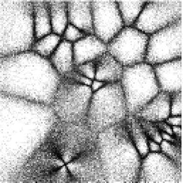
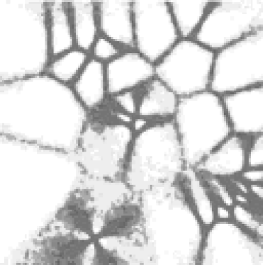
Consider the distribution and Gaussians shown in Figure 2. What happens when we try to estimate the underlying distribution from data? The true number of Gaussians that created this data is 27, but the EM algorithm does not know this in advance (and even if it did, there is no guarantee that running EM starting with 27 Gaussians will minimize the expected divergence between the true and estimated distribution). We show the results of doing so in Table 1.

There are a number of computational and optimization reasons for not simply increasing the number of Gaussian components until the the AIC or BIC score is minimized. Computationally choosing the best $k$ out of a range $1\ldots k_{\mbox{\scriptsize max}}$ is expensive as it costs $k_{\mbox{\scriptsize max}}$ times the computation of a single EM run. In terms of optimization even for the $k$ that would in principal be able to achieve the best score, the local-optima problem means we are unlikely to find the best configuration of Gaussians for that $k$. This can easily be seen in Figures 4 and 5 where some of the Gaussians are clearly needed in another part of space, but have no means to “push past” other Gaussians and get to their preferred locations.

To combat these problems, we use an elementary heuristic splitting procedure. (A similar algorithm, for Bayesian computations is contained in Richardson and Green, 1997.) We begin by running with one Gaussian. We then execute the following algorithm:

1. Randomly decide whether to try increasing or decreasing the number
   of Gaussians.

2. If we decide to increase...

   2.1 Randomly choose a number between 0 and 1 called SPLITFRACTION

   2.2 Some of the Gaussians will be allowed to split in two. We sort
       to Gaussians in increasing order of a quantity known as SPLITCRITERION.

   2.3 The best N Gaussians according to this criterion are allowed
       to split, where N = SPLITFRACTION * Total Number of Gaussians

   2.4 Each splitting Gaussian is divided into two, by making two copies
       of the original, squashing the covariance to become thinner in the
       direction of the principal component of the original covariance
       matrix, and then pushing one copy’s mean a short distance in one
       direction along this component and the other copy’s mean in the other
       direction. Figure 1 shows an example.

3. If we decide to decrease...

   3.1 Randomly choose a number between 0 and 1 called KILLFRACTION

   3.2 Some of the Gaussians will be deleted. We sort
       to Gaussians in increasing order of a quantity known as KILLCRITERION.

   3.3 The worst N Gaussians according to this criterion are deleted
       where N = KILLFRACTION * Total Number of Gaussians

4. Then, whether or not we decided to increase or decrease, we run EM
   to convergence from the new mixture. We then look at the model scoring
   criterion (AIC, BIC or testset) for the resulting mixture. Is it better
   than the original mixture?

5. If it’s better...

   5.1 We restart a new iteration with the new mixture and jump to Step 1.

6. If it’s worse...

   6.1 We revert to the mixture we had at the start of the iteration and
       jump to Step 1.

In the following experiments, SPLITCRITERION and KILLCRITERION are very simple: we split Gaussians with relatively high mixture probabilities and we kill Gaussians with relatively low mixture probabilities. We have performed experiments (not reported here) with alternative, and occasionally exotic, criteria, but find that the simple approach reported here is generally reasonable.

This approach benefits from searching through many values of $k$ in large steps, and so is faster, But more importantly it removes some of the local minima problems, so that a suboptimal local optimum with $k$ centers may manage to move to a superior solution with $k$ centers by means of an intermediate step at which useful new centers are added, iterated, and then less useful centers are deleted.

4 Applications to Astrophysical problems

We consider here two astrophysical applications of the density estimation techniques presented in this paper to illustrate their potential (though as we note below there are a large number of applications that would benefit from this approach). In the next section we apply mixture models to the reconstruction of the density distribution of galaxies from photometric and spectroscopic surveys. In the subsequent sections we discuss the application of mixtures to modeling the distribution of stellar colors in order to identify objects with anomalous colors (e.g. searching for high redshift QSOs).

4.1 Reconstructing the Density Distribution of Galaxies

Observations of the distributions of galaxies have shown that the dominant large-scale features in the Universe are comprised of walls and voids (Geller and Huchra 1990, Broadhurst et al. 1990). These structures exist over a wide range of scales, from filaments that are a few h^-1 Mpc across to walls that extend across the size of the largest surveys we have undertaken. The consequence of this is that any technique that is used to measure the density distribution must be able to adapt to this range of scales.

In this section we compare the EM algorithm, as presented in this paper, to a more traditional kernel–smoothing density estimator. For this comparison, we use simulated data sets generated from a Voronoi Tessellation since the observed distribution of filaments and sheets of galaxies in the universe can be reasonably well simulated using such a distribution. In this scenario the walls of the foam are considered as the positions of the filaments and the underdense regions between these walls the position of the voids. This simulation provides a very natural description of structure formation in the Universe as a Voronoi distribution arises when mass expands away from a set of points until it collides with another overdensity and ceases expanding.

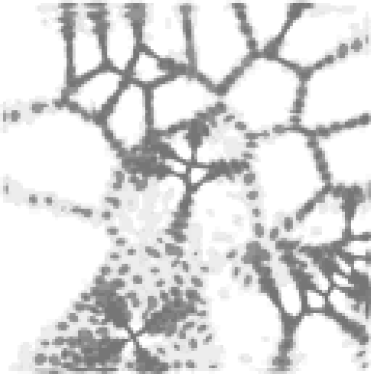
In Figure 8, we present the underlying Voronoi density map we have constructed; this is the “truth” in our simulation (the top–left panel). From this distribution we derive a set of 100,000 data points to represent a mock 2-dimensional galaxy catalog (top–right panel). We note here we have not added any additional noise to this mock galaxy catalog so it is an over–simplification of a real galaxy survey which would have “fingers–of–God” and measurement errors.

We have applied the EM algorithm (with both the AIC and BIC splitting criteria) and a standard fixed kernel density estimator to these point-like data sets in order to reproduce the original density field. The latter involved finely binning the data and smoothing the subsequent grid with a binned Gaussian filter of fixed bandwidth which was chosen by hand to minimize the KL divergence between the resulting smoothed map and the true underlying density distribution (i.e.  to minimize the difference between the top–left and the bottom-left panels in Figure 8. Clearly, we have taken the optimal situation for the fixed kernel estimator since we have selected it’s bandwidth to ensure as close a representation of the true density distribution as possible. This would not be the case in reality since we would never known the underlying distribution and would thus be forced to choose the bandwidth using various heuristics.

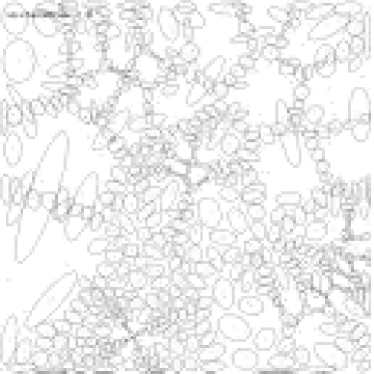
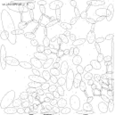
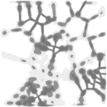
The lower left panel of Figure 8 shows the reconstructed density field using the fixed kernel and the lower right panel the corresponding density field derived from the EM algorithm using the AIC criterion. As we would expect the fixed kernel technique provides an accurate representation of the overall density field. The kernel density map suffers, however, when we consider features that are thinner than the width of the kernel. Such filamentary structures are over-smoothed and have their significance reduced. In contrast the EM algorithm attempts to adapt to the size of the structures it is trying to reconstruct. The lower right panel shows that where narrow filamentary structures exist the algorithm places a large number of small Gaussians. For extended, low frequency, components larger Gaussians are applied. The overall result is that the high frequency components (e.g. sharp edges) present within the data are reproduced accurately with out the smoothing of the data seen in the fixed kernel example.

To quantify these statements we use the KL divergence to test the similarity between the different maps. For the fixed kernel estimator, we measure a KL divergence of 0.074 between the final smoothed map and the true underlying density map (remember, this is the smallest KL measurement by design). For the EM AIC density map we measure a KL divergence of 0.067 which is lower than the best fixed kernel KL score thus immediately illustrating the power of the EM methodology. We have not afforded the same prior knowledge to the EM measurement – i.e.  hand–tune it so as to minimize the KL divergence – yet we have beaten the kernel estimator. For reference, the EM BIC estimator scored 0.078 and a uniform distribution scored 2.862 for the KL divergence with the true underlying density distribution.

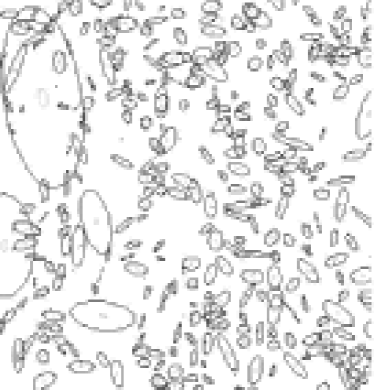
In Figure 9, we compare the relative performances of the EM AIC (top two panels) and BIC (lower two panels) criteria. The left hand side of the figure shows the centers, sizes and orientations of the Gaussians that are used to reconstruct the density distribution. The right hand panel shows the reconstructed density field derived from these Gaussians. The AIC criteria under smooths the data using a larger number of small Gaussians to reproduce the observed density field. While this better traces the small narrow features within the data it is at the cost of a larger number of components (and consequently a loss in the compactness of the representation of the data). BIC in contrast converges to a smaller number of Gaussians and a more compact representation. The fewer components (typically larger Gaussians) do not trace the fine structure in the data.

4.1.1 Application to the Las Campanas Redshift Survey

Extending the analysis in Section 4.1 to the case of the spatial distribution of galaxies, we consider the distribution of galaxies taken from the Las Campanas Redshift Survey (LCRS; Shectman et al. 1996). The LCRS comprises of a spectroscopic and photometric survey of over 26,000 galaxies selected from six regions of the sky. Each region comprises of a slice on the sky approximately 1.5 degrees thick and 80 degrees wide. With a mean redshift of $z=0.1$, the depth of this survey is approximately 300 h^-1 Mpc. Details of the selection function for the LCRS, the distribution of galaxies on the sky and how this survey was constructed can be found in Shectman et al. (1996) and Lin et al. (1996).

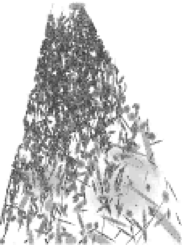
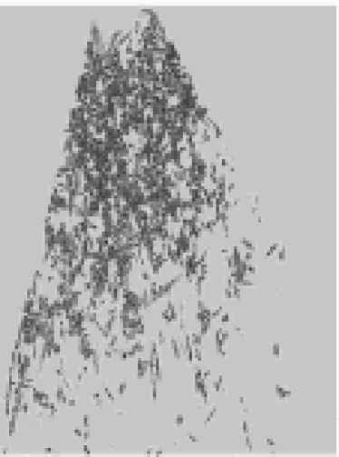
For the purpose of our analysis, we select a subset of the LCRS data which is the co–addition of the data in the three “northern” slices of the survey (slices at $-3^{\circ}$, $-6^{\circ}$ & $-12^{\circ}$ in declination). Moreover, we have ignored the thickness of the slice and converted the original spherical coordinates to a two–dimensional Euclidean coordinate system. We limited the analysis to a box $100\times 150$h^-1 Mpc in size taken from this data which contained 11195 galaxies in total; the distribution of these galaxies is shown as (red) data points in Figure 10 along with our EM analysis of these data.

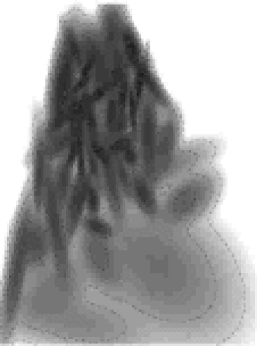
The density maps (grayscales) shown in Figure 10 were obtained by running the EM algorithm for 2 hours on a 600MHz PentiumIII machine with 128 MBytes of memory. In Figure 11, we show the AIC score found by the EM algorithm as a function of run time. The algorithm asymptotically approaches the best AIC score while checking for local minima along the way (the ends of the error bars in Figure 11 show the starting and end AIC score after one iteration of splitting procedure). For this case, we have used a splitting probability of 0.125 and fixed the number of sub-iterations to be five, i.e.  the algorithms continues for 5 iterations along a given branch before determining if this iteration has worsened the overall AIC score. If so, the EM algorithm returns to the original Gaussian centroids and tries again. This behavior is clearly seen in 11 where in some cases the ending AIC (top of the error bar) is substantially worse than the beginning AIC score. Therefore, this heuristic splitting algorithm ensures we approach the true minimum AIC score in less than approximately 20 minutes for over 10,000 data points.

Figure 10 demonstrates the adaptive nature of EM. Here we discuss practical issues of applying the EM algorithm to the LCRS data; we present results of three different runs of the EM algorithm with different initial conditions i.e.  AIC, BIC and AIC plus a uniform background. We do not present the combination of BIC and a uniform background since in all cases the EM algorithm quickly iterated to zero uniform background for these data. In the case of AIC scoring with no uniform background, the EM algorithm provides an accurate representation of the data. Our only concern is that the algorithm has potentially under-smoothed the data and does exhibit a fraction of highly elongated Gaussians. These issues we explored in section 4.1 where we demonstrated that EM AIC was better than even than the best kernel density estimator and also possessed highly elongated Gaussians. These problems are lessened in the case of AIC plus a uniform background but in this case, it does not accurately represent the low density areas of the data which are probably better described using a higher order functional form for the background rather than the uniform component assumed here. In the case of BIC, EM appears to have over-smoothed the data. It gives an accurate representation of the large–scale structure in the data, but no information on the small-scale structure.

In summary, the combination of AIC, BIC and some large–scale slowly varying smooth background should provide the best representation of the LCRS data. This should be possible to implement since: a) we can modify the penalized likelihoods as we wish – Abramovich et al. (2000) have recently proposed $\lambda_{k}=\log(\frac{R_{k}}{n})$ as a new penalized likelihood that appears to live between the two extremes of BIC and AIC (this will be explored in a future paper); b) we can add more terms to the uniform background component of the mixture model. Specifically, we could initially compress the data into a single redshift histogram and fit a low–order polynomial to this distribution and use that as the initial background for the EM algorithm. Alternatively, the large scale shape of the redshift histogram is governed by selection effects; at low redshift it is simply the volume increasing (as $z^{2}$) while at large redshifts it is due to the magnitude limit which cuts–off the luminosity function. These effects could be modelled and used as the initial background.

In Figure 12, we present a thresholded EM density map for both AIC and BIC. The threshold corresponds to a $3\sigma$ probability limit for these mixture models of Gaussian i.e.  a probability of greater than 0.001. This shows the ability of EM to accurately characterize highly non–linear hierarchical structures by inverting the point source data to obtain the underlying density distribution. This figure again illustrates the advantage of merging these two representations of the density field since the BIC gives an excellent representation of the large–scale structure, while the AIC encapsulates the higher–order structure.

4.2 Classification of Multicolor Data

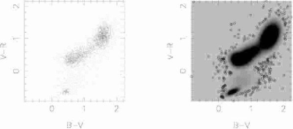
The EM algorithm is more generally applicable to density estimation problems in astrophysics than the standard spatial clustering analyses that we have discussed previously. We demonstrate this by applying EM to the question of how to identify anomalous records in multidimensional color data (e.g. the identification of high redshift QSOs from color-color diagrams). In Figure 13 we show the distribution of 6298 stellar sources in the B-V and V-R color space (with R$<$22) taken from a 1 sq degree multicolor photometric survey from Szokoly et al (2000). Applying the EM algorithm using the AIC scoring criteria we derive the density distribution for the B-V – V-R color space. The grayscale image on Figure 13 shows the resultant mixture density map. As we would expect from the results from our analysis of the spatial distribution of galaxies in the LCRS the EM distribution traces the stellar locus with the most dense regions on this map reflecting the distribution of M stars.

¿From the mixture density distribution we define a probability density map. This gives the probability that a stellar object drawn at random from the observed distribution of stars would have a particular set of B-V – V-R colors. We can now assign a probability to each star in the original data that describes the likelihood that it arises from the overall distribution of the stellar locus. We can then rank order all sources based on the likelihood that they were drawn from the parent distribution. The right panel of Figure 13 shows the colors of the 5% of sources with the lowest probabilities. These sources lie preferentially away from the stellar locus. As we increase the cut in probability the colors of the selected sources move progressively closer to the stellar locus.

The advantage of the mixture approach over standard color selection techniques is that we identify objects based on the probability that they lie away from the stellar locus (i.e. we do not need to make orthogonal cuts in color space as the probability contours will trace accurately the true distribution of colors). While for two dimensions this is a relatively trivial statement as it is straightforward to identify regions in color–color space that lie away from the stellar locus (without being restricted to orthogonal cuts in color-color space) this is not the case when we move to higher dimensional data. For four and more colors we lose the ability to visualize the data with out projecting it down on to a lower dimensionality subspace (i.e. we can only display easily 3 dimensional data). In practice we are, therefore, limited to defining cuts in these subspaces which may not map to the true multidimensional nature of the data. The EM algorithm does not suffer from these disadvantages as a probability density distribution can be defined in an arbitrary number of dimensions. It, therefore, provides a more natural description of both the general distribution of the data and for the identification of outlier points from high dimensionality data sets. With the new generation of multi-frequency surveys we expect that the need for algorithms that scale to a large number of dimensions will become more apparent.

5 Discussion & Conclusions

With the current and future generation of wide-angle, multi-frequency surveys it is becoming increasingly apparent that we need to develop new analysis techniques that scale to the domain of large numbers of objects and multiple dimensions (e.g. colors). In this paper we have presented one such statistical approach; the use of Mixture Models in the density estimation of large astronomical datasets. Implementing Mixture Models under a multi–resolution KD–tree framework we have developed a fast, adaptive density estimator that can accurately recover the underlying density distribution from point processes.

Applying these techniques to simulated galaxy redshift catalogs we find that the EM algorithm provides a better representation of the underlying density distributions than the best-case fixed-kernel density estimators. We find that different scoring criteria for determining the accuracy of the density estimation provide different final representations of the underlying density. The BIC method produces a smooth, compact representation of the data while AIC better reflects high frequency components within the data with the associated loss in compactness (i.e. an increased number of Gaussians).

We demonstrate the broad class of astrophysical problems that would benefit from such approach by considering two distinct cases; the clustering of galaxies in redshift space using the LCRS data set and the clustering of stars in color space to identify objects of unusual color. We find that the adaptive nature of the EM algorithm enables an accurate description of both the low and high frequency components within the LCRS data. As with the simulated data sets using the BIC scoring results in an apparent under-smoothing of the data while the AIC score produces a better representation of the high frequency modes at the cost of requiring a larger number of Gaussians to describe the data. A hybrid scoring criteria that mixes the properties of AIC and BIC may provide the most accurate representation.

For applications to clustering in color space the results are equally encouraging. As the result of the EM algorithm is a density map that can be expressed in terms of the probability than an object would have a particular set of colors EM provides a simple and intuitive approach to identifying outliers within this color space. It can be implemented for data of an arbitrary number of dimensions (and parameters) and is therefore well suited to observations taken over a wide spectral range.

To date we have only considered here a mixture model of Gaussians. It is mathematically straightforward to consider a mixture of any profiles one desires. The price one may pay in that case is in efficient computation. Two astronomically interesting profiles we may try are the Plummer or isothermal profile for identifying clusters of galaxies – which has been used in automated searches for clusters of galaxies – and the double Gaussian profile which is typically used to create a Gaussian–like profile but with long wings. The latter has been used to describe the point–spread function of the Sloan Digital Sky Survey as well as other telescopes and instruments. We plan to explore these other mixture models in future papers.

To facilitate the use of EM in astronomical data-analysis, a version of the software used herein (FASTMIX) can be obtained from http://www.cs.cmu.edu/ÃUTON/applications.html. At present, only a Linux binary executable of the software has been made available but encourage people to contact us directly if they wish to examine the source code or require a binary built for a different operating system (email: nichol@cmu.edu).

Appendix A Derivation of the EM algorithm

For the readers convenience, we include here a derivation of the EM algorithm for the mixture model. For simplicity of presentation, we omit the uniform component in what follows. The idea is to define a random variables $Z$ such that $f(x;\theta)=\int f(x,z;\theta)dz$ and such that maximizing the complete data likelihood based on the $X_{i}^{\prime}s$ and the $Z_{i}^{\prime}s$ is easy. We define $Q$ to be the expected value (over $Z$) of the complete data log-likelihood. We iterate between computing $Q$ and maximizing $Q$ For details, see Dempster, Laird and Rubin (1977). Here are the details for mixtures.

Define $Z_{ij}=1$ if $Y_{i}$ is from group $j$ and $Z_{ij}=0$ otherwise. The log-likelihood of $Y_{i}^{\prime}s$ and the $Z_{ij}^{\prime}s$ is called the complete log-likelihood and is given by $\ell=\sum_{j}\sum_{i}Z_{ij}[\log p_{j}+\log\phi(Y_{i};\mu_{j},\Sigma_{j})]$. Let $\tilde{\theta}$ represent the current guess at the parameters. Define

$$Q = E(\ell|Y^{n},\tilde{\theta})$$

$$= \sum_{j}\sum_{i}E(Z_{ij}|Y^{n},\tilde{\theta})[\log\tilde{p}_{j}+\log\phi(Y_{i};\tilde{\mu}_{j},\tilde{\Sigma}_{j})]$$

$$= \sum_{j}\sum_{i}\tau_{ij}[\log\tilde{p}_{j}+\log\phi(Y_{i};\tilde{\mu}_{j},\tilde{\Sigma}_{j})]$$

where,

$$\tau_{ij} = E(Z_{ij}|Y^{n},\tilde{\theta})$$

$$= Pr(Y_{j}\ {\rm is\ in\ group\ j}|Y^{n},\tilde{\theta})$$

$$= \frac{f(y_{i}|{\rm group\ j})Pr({\rm group\ }j)}{\sum_{r}f(y_{i}|{\rm group\ r})Pr({\rm group\ }r)}$$

$$= \frac{\tilde{p}_{j}\phi(y_{i};\tilde{\mu}_{j},\tilde{\Sigma}_{j})}{\sum_{r}\tilde{p}_{r}\phi(y_{i};\tilde{\mu}_{r},\tilde{\Sigma}_{r})}$$

by Bayes’ theorem.

Now, using the definition of a Gaussian, we have

$$Q = \sum_{j}\sum_{i}\tau_{ij}[\log p_{j}+\log\phi(Y_{i};\mu_{j},\Sigma_{j})]$$

$$= \sum_{j}\log p_{j}\sum_{i}\tau_{ij}-\frac{1}{2}\sum_{j}\sum_{i}\tau_{ij}\log det\Sigma_{j}-\frac{1}{2}\sum_{j}\sum_{i}\tau_{ij}(Y_{i}-\mu_{j})^{T}\Sigma_{j}^{-1}(Y_{i}-\mu_{j})$$

$$= \sum_{j}\tau_{\cdot j}\log p_{j}-\frac{1}{2}\sum_{j}\tau_{\cdot j}\log det\Sigma_{j}-\frac{1}{2}\sum_{j}\sum_{i}\tau_{ij}(Y_{i}-\mu_{j})^{T}\Sigma_{j}^{-1}(Y_{i}-\mu_{j}).$$

where $\tau_{\cdot j}=\sum_{i}\tau_{ij}$. Let

$$\hat{\mu}_{j}=\frac{\sum_{i=1}^{n}\tau_{ij}Y_{i}}{\tau_{\cdot j}}.$$

Note that $\sum_{j}\sum_{i}\tau_{ij}(Y_{i}-\hat{\mu}_{j})^{T}\Sigma_{j}^{-1}(\hat{\mu}_{j}-\mu_{j})=0$. Also, let $trA$ denote the trace of the matrix $A$. Recall that if $A$ is symmetric then $x^{T}Ax=tr(Ax^{T}x)$. Also, $tr(\sum_{i}A_{i})=\sum_{i}tr(A_{i})$. Therefore,

$$\sum_{j}\sum_{i}\tau_{ij}(Y_{i}-\mu_{j})^{T}\Sigma_{j}^{-1}(Y_{i}-\mu_{j}) = \sum_{j}\sum_{i}([Y_{i}-\hat{\mu}_{j}]+[\hat{\mu}_{j}-\mu_{j}])^{T}\Sigma_{j}^{-1}([Y_{i}-\hat{\mu}_{j}]+[\hat{\mu}_{j}-\mu_{j}])$$

$$= \sum_{j}\sum_{i}\tau_{ij}(Y_{i}-\hat{\mu}_{j})^{T}\Sigma_{j}^{-1}(Y_{i}-\hat{\mu}_{j})+\sum_{j}\tau_{\cdot j}(\hat{\mu}_{j}-\mu_{j})^{T}\Sigma_{j}^{-1}(\hat{\mu}_{j}-\mu_{j})$$

$$= \sum_{j}\sum_{i}tr\left\{\tau_{ij}\Sigma_{j}^{-1}(Y_{i}-\hat{\mu}_{j})(Y_{i}-\hat{\mu}_{j})^{T}\right\}+\sum_{j}\tau_{\cdot j}(\hat{\mu}_{j}-\mu_{j})^{T}\Sigma_{j}^{-1}(\hat{\mu}_{j}-\mu_{j})$$

$$= \sum_{j}tr\left(\Sigma_{j}^{-1}B_{j}\right)+\sum_{j}\tau_{\cdot j}(\hat{\mu}_{j}-\mu_{j})^{T}\Sigma_{j}^{-1}(\hat{\mu}_{j}-\mu_{j})$$

where

$$B_{j}=\sum_{i}\tau_{ij}(Y_{i}-\hat{\mu}_{j})(Y_{i}-\hat{\mu}_{j})^{T}.$$

Hence,

$$Q=\sum_{j}\tau_{\cdot j}\log p_{j}-\frac{1}{2}\sum_{j}\tau_{\cdot j}\log det\Sigma_{j}-\frac{1}{2}\sum_{j}tr\left(\Sigma_{j}^{-1}B_{j}\right)-\frac{1}{2}\sum_{j}\tau_{\cdot j}(\hat{\mu}_{j}-\mu_{j})^{T}\Sigma_{j}^{-1}(\hat{\mu}_{j}-\mu_{j}).$$

Now we need to maximize $Q$ subject to $\sum_{j}p_{j}=1$. Take the derivative with respect to $p_{j}$ and set equal to 0 to conclude that the root satisfies

$$\hat{p}_{j}=\frac{\sum_{i}\tau_{ij}}{n}.$$

Note that $\mu_{j}$ appears only in the last term. This term is non-positive and is clearly maximized by setting $\mu_{j}=\hat{\mu}_{j}$. It remains then to find $\Sigma_{j}$ to maximize

$$-\frac{1}{2}\sum_{j}\tau_{\cdot j}\log det\Sigma_{j}-\frac{1}{2}\sum_{j}tr\left(\Sigma_{j}^{-1}B_{j}\right).$$

Taking exponentials, note that this is the same as maximizing

$$\sum_{j}\frac{1}{(det\Sigma_{j})^{\tau_{\cdot j}/2}}\exp\left\{-\frac{1}{2}tr\left(\Sigma_{j}^{-1}B_{j}\right)\right\}.$$ (A1)

In general, if $B$ is a $d\times d$ symmetric, positive definite matrix and $b>0$ then

$$\frac{1}{(det(\Sigma))^{b}}\exp\left\{-\frac{1}{2}tr(\Sigma^{-1}B)\right\}\leq\frac{1}{(det(B))^{b}}(2b)^{db}e^{-bd}$$

with equality if and only if $\Sigma=B/(2b)$. It follows that (A1) is maximized by

$$\hat{\Sigma}_{j}=\frac{B_{j}}{\tau_{\cdot j}}.$$

Table 1: Comparison of AIC and BIC scoring algorithms

Scoring Criterion	BIC	AIC
Num Gaussians in Best Model	33	54
KL-Divergence to true distribution	0.207	0.067
Seconds to compute using traditional EM	XXX ?	XXX ?
Seconds to compute using MRKD-trees	450	450
Drawing of Gaussian in best model	Figure 4	Figure 5
Drawing of PDF of best model	Figure 6	Figure 7

Figure 1: The rectangle denotes a hyper-rectangle in the mrkd-tree. The small squares denote data points “owned” by the node. Suppose there are just two classes, with the given means, and covariances depicted by the ellipses. Small circles indicate the locations within the node for which $a_{j}$ (i.e. $P(x\mid c_{j})$) would be extremized.

Figure 2: two-dimensional Gaussian mixture. The ellipses show the two-sigma contours of the ellipses. The dots show a sample of the data from the mixture (the full dataset has 80000 points).

Figure 3: The PDF of the mixture model of Figure 2

Figure 4: The Gaussian comprising the mixture model identified from the data using a search for $k=1\ldots 60$ and the BIC criterion.

Figure 5: The Gaussian comprising the mixture model identified from the data using a search for $k=1\ldots 60$ and the AIC criterion.

Figure 6: The PDF Associated with the best BIC model of Figure 4.

Figure 7: The PDF Associated with the best AIC model of Figure 5.

Figure 8: A comparison of the fixed kernel and EM density estimation techniques. The top left panel shows the simulated density distribution drawn from a Voronoi Tessellation. The top right panel shows a data set of 100,000 data points drawn from the Voronoi distribution. The results of density estimation are given in the lower two panels with the left panel showing a fixed kernel density estimation (where the kernel has been “hand tuned” to provide the most accurate representation of the data – see text) and the right panel the density derived from the EM algorithm using AIC scoring. The fixed-kernel and EM algorithms both reproduce accurately the broad features within the simulated data. The EM algorithm does, however, adapt to the sharpest features in the data whereas the fixed kernel over smooths these regions.

Figure 9: A comparison of the density estimation using the AIC and BIC scoring criteria when applied to the Voronoi simulation. The top two panels show the distribution of Gaussians (left) produced by EM using the AIC score and the resulting density distribution (right). The lower two panels show the same distributions but for the BIC scoring criterion. The AIC scoring clearly results in a larger number of Gaussians which better represent the small scale features within the data (but with a corresponding loss in the compactness of the description of the data). In comparison the BIC scoring results in many fewer Gaussians but does not trace the fine structure as accurately.

Figure 10: The EM probability density maps (normalized to an integrated probability of unity) for the LCRS data discussed in the text. The top–left panel is for AIC scoring while the top–right panel is for BIC scoring. The bottom–left panel is a small subset of the data plus fitted Gaussians taken from the AIC scoring run presented in full in the top–left panel. The bottom-right panel shows the AIC scoring run but with a uniform background component in the mixture model. All three runs used the same splitting probability (0.125) and were run for 2 hours on a 600MHz PentiumIII with 128 MBytes of memory (although as illustrated in Figure 11, EM converges to a solution in less than 20 minutes).

Figure 11: The EM AIC score for the LCRS data as a function of time (seconds). Each point is presented as an error bar where the top of the bar represents the AIC after one splitting iteration, while the bottom is the beginning AIC score.

Figure 12: A thresholded map of EM AIC (top) and BIC (bottom).

Figure 13: The application of EM to d ensity estimation in color space. The left panel shows the distribution of $B-V$ and $V-R$ colors of stellar sources. The right hand panel shows the density distribution, in grayscale, of these sources derived from the EM algorithm (using the AIC scoring criterion) together with the 5% of the data that is least likely to be drawn from this distribution (open circles).

References

- (1)
- (2) Abramovich, F., Benjamini, Y., Donoho, D., Johnstone, I. (2000). “Adapting to Unknown Sparsity by Controlling the False Discovery Rate”, Technical Report, Statistics Department, Stanford University.
- (3)
- (4) Akaike, H. (1973). Proceedings of “Second International Symposium on Information Theory”, ed. Petrov, B.N., Caski, F., 267
- (5)
- (6) Banfield, J.D., Raftery, A. E., 1993, Biometrics, 49, 803
- (7)
- (8) Barron, A., Yang, Y., 1995, “An asymptotic property of a model selection criterion”, Technical report, Statistics Department, Yale University.
- (9)
- (10) Barron, A., Birge, L., Massart, P., 1999, Probability Theory and Related Fields, 113, 3, 301
- (11)
- (12) Broadhurst, T. J., Ellis, R. S., Koo, D. C., Szalay, A. S., 1990, Nature, 343, 726
- (13)
- (14) Burman, P., 1989, Biometrika, 76, 503
- (15)
- (16) Dacunha-Castelle, D., Gassiat, E., 1996, “Testing the order of a model using locally conic parameterization: population mixtures and stationary ARMA processes”, Technical report
- (17)
- (18) Dempster, A., Laird, N., Rubin, D., 1977, Journal of the Royal Statistical Society, 39, 1
- (19)
- (20) Deng, K., Moore, A. W., 1995, Proceedings of “The Twelfth International Joint Conference on Artificial Intelligence”
- (21)
- (22) Donoho, D., Johnstone, I., Kerkyacharian, G., Picard, D., 1996, The Annals of Statistics, 24, 508
- (23)
- (24) Fraley, C., Raftery, A. E., 1998, “How many clusters? Which clustering method? - Answers via Model-Based Cluster Analysis”, Technical Report no. 329, Department of Statistics, University of Washington.
- (25)
- (26) Geller, M., Huchra, J., 1990, Scientific American, 262, 19
- (27)
- (28) Genovese, C., Wasserman, L. (1998). “Rates of convergence for the Gaussian mixture sieve”, Technical report, Department of Statistics, Carnegie Mellon University
- (29)
- (30) Hartigan, J., 1975, “Clustering Algorithms”, Wiley, New York
- (31)
- (32) Hartigan, J., 1987, Journal of the American Statistical Association, 82, 267
- (33)
- (34) Keribin, C., 1999, “Consistency of penalized likelihood for mixture models”, Ph.D. thesis, Department of Mathematics, University of Paris
- (35)
- (36) Lin, H., Kirshner, R. P., Shectman, S. A., Landy, S. D., Oemler, A., Tucker, D. L., Schechter, P. L., 1996, ApJ, 464, 60
- (37)
- (38) McLachlan, G., Basford, K., 1988, “Mixture Models. Inference and Applications to Clustering”, Marcel Dekker, New York.
- (39)
- (40) Moore, A. W., Schneider, J., Deng, K., 1997, Proceedings of “The Fourteenth International Conference on Machine Learning”, ed. Fisher, D.,
- (41)
- (42) Moore, A. W., 1999, Proceedings of “Advances in Neural Information Processing Systems 10”, ed. Kearns, M., Cohn, D.,
- (43)
- (44) Müller, D., Sawitzki, G., 1991, Journal of the American Statistical Association, 86, 738
- (45)
- (46) Nolan, D., 1991, Journal of Multivariate Analysis, 39, 348
- (47)
- (48) Polonik, W., 1995, The Annals of Statistics, 23, 855
- (49)
- (50) Richardson, S., Green, P.J., 1997, Journal of the Royal Statistical Society, 59, 731
- (51)
- (52) Roeder, K., Wasserman, L., 1997, Journal of the American Statistical Association, 92, 894
- (53)
- (54) Schwarz, G., 1978. Annals of Statistics, 6, 461
- (55)
- (56) Shao, J., 1993, Journal of the American Statistical Association, 88, 486,
- (57)
- (58) Shectman, S A., Landy, S. D., Oemler, A., Tucker, D. L., Lin, H., Kirshner, R. P., Schechter, P L., 1996, ApJ, 470, 172
- (59)
- (60) Silverman, B., 1986, “Density Estimation For Statistics and Data Analysis”, Chapman & Hall, New York.
- (61)
- (62) Smyth, P., 1996, Proceedings of “The 2nd International Conference on Knowledge Discovery and Data Mining”, AAAI Press
- (63)
- (64) Szalay, A. S., Brunner, R.J., “Astronomical Archives of the Future: A Virtual Observatory”. Published in ”Future Generation Computer Systems” (see astro-ph/9812335)
- (65)
- (66) Szoloky, G., et al. (2000), in preparation.
- (67)
- (68) van der Vaart, A., 1998, “Asymptotic Statistics”, Cambridge University Press, Cambridge.
- (69)
- (70) York, D. G. et al. (2000), ApJ, accepted (see astro-ph/0006396)