Towards a refined cosmic concordance model: joint 11-parameter constraints from CMB and large-scale structure

Abstract

We present a method for calculating large numbers of power spectra $C_{\l}$ and $P(k)$ that accelerates CMBfast by a factor around $10^{3}$ without appreciable loss of accuracy, then apply it to constrain 11 cosmological parameters from current Cosmic Microwave Background (CMB) and Large Scale Structure (LSS) data. While the CMB alone still suffers from several degeneracies, allowing, e.g., closed models with strong tilt and tensor contributions, the shape of the real space power spectrum of galaxies from the IRAS Point Source Catalogue Redshift (PSCz) survey breaks these degeneracies and helps place strong constraints on most parameters. At 95% confidence, the combined CMB and LSS data imply a baryon density $0.020<\omega_{\rm b}<0.037$, dark matter density $0.10<\omega_{\rm dm}<0.32$ with a neutrino fraction $f_{\nu}<38\%$, vacuum density $\Omega_{\Lambda}<0.76$, curvature $-0.19<\Omega_{\rm k}<0.10$, scalar tilt $0.86<n_{s}<1.16$, and reionization optical depth $\tau<0.44$. These joint constraints are quite robust, changing little when we impose priors on the Hubble parameter, tilt, flatness, gravity waves or reionization. Adding nucleosynthesis and neutrino priors on the other hand tightens constraints considerably, requiring $\Omega_{\Lambda}>0.49$ and a red-tilt, $n_{s}<1$.

The analysis allows a number of consistency tests to be made, all of which pass. At the 95% level, the flat scalar “concordance model” with $\Omega_{\Lambda}=0.62$, $\omega_{\rm dm}=0.13$, $\omega_{\rm b}=0.02$, $f_{\nu}\sim 0$, $n_{s}=0.9$, $\tau=0.1$, $h=0.63$ is consistent with the CMB and LSS data considered here, with big bang nucleosynthesis, cluster baryon fractions and cluster abundance. The inferred PSCz bias $b\sim 1.2$ agrees with the value estimated independently from redshift space distortions. The inferred cosmological constant value agrees with the one derived independently from SN 1a studies. Cosmology seems to be on the right track!

]

FIG. 1.: The importance of including non-CMB information. The best fit to all current CMB data (solid curve) is still a crazy tilted model ($n_{s}=1.4$) for a closed universe ($\Omega_{\rm tot}=1.3$) with the COBE signal explained almost entirely with tensor fluctuations. The dashed curves show the tensor and scalar contributions.

I INTRODUCTION

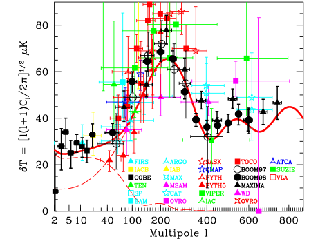
The cosmic microwave background (CMB) is dramatically improving our knowledge of cosmological parameters [1, 2, 3, 4, 5, 6], although as can be seen in Figure 1, the constraints from CMB alone are weaker than is sometimes claimed. The figure shows that the adiabatic inflationary model that fits the CMB data best is still a crazy one with extreme scalar tilt $n_{s}=1.4$, curvature ($\Omega_{\rm tot}=1.3$) and the COBE signal explained almost entirely with tensor fluctuations (gravity waves).

Indeed, CMB data have now become so sensitive that the key issue in cosmological parameter determination is not always the accuracy with which CMB power spectrum features (such as the position of the first peak) can be measured, but often what prior information is used or assumed (e.g., that there are no tensor fluctuations). A range of priors were explored in recent studies [1, 2, 3, 4, 5, 6], including assumptions about reionization and gravity waves and constraints from nucleosynthesis, supernovae, large-scale structure and the Hubble constant. In particular, two extensive multiparameter analyses [1, 5] included large-scale structure (LSS) information as quantified by a normalization and the so-called “shape parameter” $\Gamma$ (which slides a fixed transfer function sideways) from galaxy power spectrum measurements and cluster abundances, extending earlier CMB+LSS work [7, 8, 9, 10, 11, 12, 13, 14, 15, 17, 18].

While much of the information in the galaxy power spectrum is indeed encapsulated in a horizontal and a vertical offset, all of it is clearly not. It should therefore be possible to do still better by fitting directly to the LSS data, explicitly including the way in which each of the cosmological parameters affect this curve, just as is presently done for the CMB. This is the goal of the present paper. Now is a particularly exciting time to start doing this, since projects like the 2dF Survey and the Sloan Digital Sky Survey will soon produce dramatic improvements in LSS data quality.

The LSS data used in this paper is the linear real space power spectrum of the IRAS Point Source Catalogue Redshift Survey [19] (PSCz) as measured by [20] and as shown in Figure 2. The PSCz survey contains redshifts for 14,677 galaxies covering 84% of the sky to a usable depth of about $400\,h^{-1}{\rm Mpc}$. Although other large data sets such as the Las Campanas Redshift Survey [21] and the CfA/SSRS UZC redshift survey [22] have comparable numbers of galaxies, the large volume of the PSCz, along with the careful attention paid by its authors to uniformity of selection, makes PSCz the most powerful publicly available probe of LSS at large, linear scales.

FIG. 2.: Why LSS data adds information to the CMB. The wiggly curve corresponds the best fit model from CMB alone that was shown in Figure 1, normalized on small scales (it has bias $b=0.5$). The straighter curve shows Prior P5 from [5] — the difficulty in matching the largest scales illustrates that there is already more information in the curve than a normalization and a shape parameter. Of the PSCz measurements shown, we opt to use only those in the fairly linear regime $k<0.3\,h\,{\rm Mpc}^{-1}$ (black), discarding the rest.

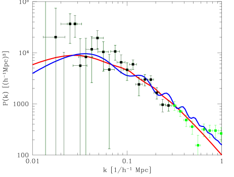
Afficionados may notice that the error bars on the PSCz power spectrum in Figure 2 appear somewhat larger than some other published measurements. This is because the measurements have been decorrelated [23] so that each plotted point represents an essentially independent piece of information. Having uncorrelated data points, or equivalently a full covariance matrix, is prerequisite for a reliable likelihood analysis.

A longstanding obstacle to interpreting LSS measurements is the thorny issue of galaxy-to-mass bias. Local bias models predict that the bias factor should be constant at large, linear scales [24, 25, 26, 27], and $N$-body experiments tend to confirm this notion [28, 29, 30, 31]. The simple situation at linear scales contrasts with the nonlinear regime, where the afore-referenced $N$-body experiments suggest that there is likely to be substantial scale-dependent bias. For this reason, we confine the analysis of the present paper to the linear regime, $k<0.3\,h\,{\rm Mpc}^{-1}$. We return to this issue below.

We will investigate how CMB and LSS constrain cosmological parameters, both jointly and in separate ways that allow consistency checks to be made. In order to be able to study the effects of prior assumptions, this forces us to work in an 11-dimensional parameter space. To make this feasible in practice, we first need to develop and test a method for computing theoretical power spectra $C_{l}$ and $P(k)$ accurately and rapidly.

The rest of this paper is organized as follows. In Section II, we summarize our methods for computing CMB and LSS power spectra, saving the implementation details and tests of their accuracy for Appendices A, B and C. We present our constraints on cosmological parameters in Section III and discuss our conclusions in Section IV.

II METHOD

Our method is based on the one described in [32], but with a number of extensions and improvements as detailed in Appendices A, B and C. It consists of the following steps:

1. Compute power spectra $C_{\l}$ and $P(k)$ for a grid of models in our 11-dimensional parameter space.

2. Compute a likelihood for each model that quantifies how well it fits the data.

3. Perform 11-dimensional interpolation and marginalize to obtain constraints on individual parameters and parameter pairs.

Our main improvement over [32] is in step 1. As described in Appendix B, we enhance the technique for accelerated CMB power spectrum calculation so that it becomes essentially as accurate as CMBfast itself, but about $10^{3}$ times faster. We also add a simple but accurate technique to compute the grid of matter power spectra rapidly as described in Appendix C. In addition, we improve the choice of parameters and gridding from [32] as detailed in Appendix A. For the reasons given there, we use the 11 parameters

$${\bf p}\equiv(\tau,\Omega_{\rm k},\Omega_{\Lambda},\omega_{\rm dm},\omega_{\rm b},f_{\nu},n_{s},n_{t},A_{s},A_{t},b).$$ (1)

These are the reionization optical depth $\tau$, the primordial amplitudes $A_{s}$, $A_{t}$ and tilts $n_{s}$, $n_{t}$ of scalar and tensor fluctuations, a bias parameter $b$ defined as the ratio between rms galaxy fluctuations and rms matter fluctuations on large scales, and five parameters specifying the cosmic matter budget. The various contributions $\Omega_{i}$ to critical density are for curvature $\Omega_{\rm k}$, vacuum energy $\Omega_{\Lambda}$, cold dark matter $\Omega_{\rm cdm}$, hot dark matter (neutrinos) $\Omega_{\nu}$ and baryons $\Omega_{\rm b}$. The quantities $\omega_{\rm b}\equiv h^{2}\Omega_{\rm b}$ and $\omega_{\rm dm}\equiv h^{2}\Omega_{\rm dm}$ correspond to the physical densities of baryons and total (cold + hot) dark matter ($\Omega_{\rm dm}\equiv\Omega_{\rm cdm}+\Omega_{\nu}$), and $f_{\nu}\equiv\Omega_{\nu}/\Omega_{\rm dm}$ is the fraction of the dark matter that is hot. We assume that the bias $b$ is constant on large scales but make no assumptions about its value, and therefore marginalize (minimize) over this parameter before quoting constraints on the other ten.

III RESULTS

FIG. 3.: The CMB and LSS power spectra for the “concordance” model from Table 1. Animated versions of this figure, where the effect of changing one parameter at a time can be viewed, are available at www.hep.upenn.edu/$\sim$max/concordance.html. The plotted model has bias $b=1.24$, redshift distortion parameter $\beta=0.47$ and hubble parameter $h=0.63$. It provides an acceptable fit to all our data, with $\chi^{2}\approx 96$ for about $109-11=98$ degrees of freedom.

A Basic results

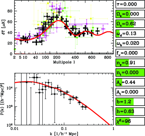
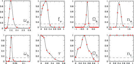
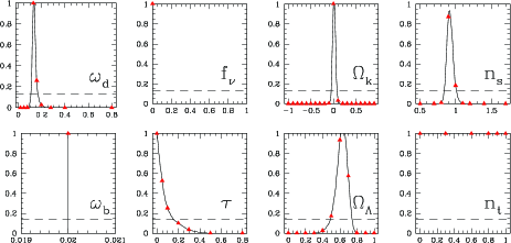
Our constraints on individual cosmological parameters are listed in Table 1 for three cases. The best fit model is shown in Figure 3 for case 3. Constraints are plotted in figures 4 and 5 for cases 2 and 3. All tabulated and plotted bounds are 95% confidence limits. The first case uses constraints from CMB alone, which are still rather weak because of degeneracy problems such as the one illustrated in Figure 1. The second case combines the CMB information with the power spectrum measurements from PSCz, and is seen to give rather interesting constraints on most parameters except the tensor tilt $n_{t}$. The third case adds three assumptions: that the latest measurements of the baryon density $\omega_{\rm b}=0.019\pm 0.0024$ from Big Bang Nucleosynthesis (BBN) are correct [34, 35], that the $1\sigma$ constraints on the Hubble parameter are $h=0.74\pm 0.08$ [36], and that the neutrino contribution is cosmologically negligible. Since the quoted BBN error bars are much smaller than our $\omega_{\rm b}$ grid spacing, we simply impose $\omega_{\rm b}=0.02$. Also for simplicity, we take the errors on $h$ to be Gaussian. The neutrino assumption is that there is no strong mass-degeneracy between the relevant neutrino families, and that the Super-Kamiokande atmospheric neutrino data therefore sets the scale of the neutrino density to be $\omega_{\nu}\sim\times 10^{-4}-10^{-3}$ [37]. We emphasize that this last assumption (that the heaviest neutrino weighs of order the root of the squared mass difference $\Delta m^{2}\sim 0.07\,{\rm eV}^{2}$) is merely motivated by Occam’s razor, not by observational evidence — the best current limits on $f_{\nu}$ from other astrophysical observations (see [38] and references therein) are still compatible with $f_{\nu}\sim 0.2$. Rather, we have chosen to highlight the consequences of this prior since, as discussed below, it has interesting effects on other parameters.

For the first 7 parameters listed in Table 1, the numbers were computed from the corresponding 1-dimensional likelihood functions (these are plotted in Figure 4 and Figure 5 for the second and third cases). The best fit value corresponds to the peak in the likelihood function and the $95\%$ limits correspond to where the likelihood function drops below the dashed line at $e^{-2}$ of the peak value. For the remaining parameters listed, which (except for $b$) are not fundamental parameters in our 11-dimensional grid, the numbers were computed as in [5] by calculating the likelihood-weighted means and standard deviations over the the multidimensional parameter space. Here the tabulated best fit values are this mean and the limits are the mean $\pm 2\sigma$.

Table 1 – Best fit values and 95% confidence limits on cosmological parameters. The “concordance” case combines CMB and PSCz information with a BBN prior $\omega_{\rm b}=0.02$, a Hubble prior $h=0.74\pm 0.08$ and a prior that $f_{\nu}\sim 10^{-3}$. A dash indicates that no meaningful constraint was obtained. The redshift space distortion parameter is $\beta\equiv f(\Omega_{\rm m},\Omega_{\Lambda})/b$, where $f$ is the linear growth rate. $z_{ion}$ is the redshift of reionization, $t_{0}$ is the present age of the Universe and $\sum m_{\nu}$ is the sum of the neutrino masses. The values labeled as “best” are in all cases the ones maximizing the likelihood. For the numbers below the horizontal line, were the limits were computed from moments as described in the text, the corresponding mean valus are $h=.53$, $z_{ion}=7$, $t_{0}=15.6$ (CMB alone), $b=1.26$, $h=.59$, $\beta=.63$, $z_{ion}=9$, $t_{0}=13.3$ (CMB+PSCz) and $b=1.10$, $h=.68$, $\beta=.51$, $z_{ion}=6$, $t_{0}=13.4$ (“concordance”). If the reader wishes to use some of these model pararameters for other purposes, the numbers to use are thus those in the table, not the ones here in the caption. Since the distributions for $\tau$ and $f_{\nu}$ are quite asymmetric, we also quote the 1-sided 95% limits $\tau<0.22$ (CMB only), $\tau<0.34$, $f_{\nu}<0.35$ (CMB+PSCz), $\tau<0.16$ (“concordance”).

	CMB alone			CMB + PSCz			Concordance
Quantity	Min	Best	Max	Min	Best	Max	Min	Best	Max
$\tau$	0.0	0.0	$0.32$	0.0	0.0	$.44$	0.0	0.0	$.16$
$\Omega_{\rm k}$	$-$.69	$-$.34	0.05	$-$.19	$-$.02	0.10	$-$.05	$-$.00	0.08
$\Omega_{\Lambda}$	$.05$	.41	$.92$	$-$	.35	0.76	.49	.62	0.74
$h^{2}\Omega_{\rm dm}$	0.0	.09	$-$	.10	.19	0.32	.11	.13	0.17
$h^{2}\Omega_{\rm b}$	.024	.049	$.103$	.020	.029	.037	.02	.02	.02
$f_{\nu}$	0.0	0.0	$1.0$	0.0	.16	.38	$\sim$0	$\sim$0	$\sim$0
$n_{s}$	.91	1.42	$-$	0.86	.98	1.16	0.84	.91	1.01
$n_{t}$	$-$	0.0	$-$	$-$	0.0	$-$	$-$	0.0	$-$
$b$	$-$	$-$	$-$	.75	1.36	1.78	.87	1.23	1.33
$h$	.18	.39	.88	.33	.57	.86	.58	.63	.78
$\beta$	$-$	$-$	$-$	.37	.59	.89	.36	.47	.66
$z_{ion}$	0	0	21	0	0	$26$	0	0	20
$t_{0}$ [Gyr]	8.4	18.0	23.0	9.6	13.1	17.0	12.1	14.0	14.6
$\sum m_{\nu}$ [eV]	0	0	17	0	2.7	7.6	$\sim$0	$\sim$0	$\sim$0

FIG. 4.: Constraints on individual parameters using only CMB and LSS information. The quoted 95% confidence limits are where each curve drops below the dashed line.

FIG. 5.: Like the previous figure, but adding the “concordance” priors $\omega_{\rm b}=0.02$, $h=0.74\pm 0.08$ and $f_{\nu}\sim 10^{-3}$.

B Effects of priors

Case 3 in Table 1 is but one from a selection of about 20 different priors that we tried experimentally. The reason that we have chosen to highlight this one is that the nucleosynthesis constraint was the one that had the greatest impact on the results. Otherwise, the joint CMB+PSZc constraints were remarkably robust to prior assumption. Imposing priors such as flatness ($\Omega_{\rm k}=0$), no tensors ($r=0$), no tilt ($n_{s}=1$), no reionization ($\tau=0$), and a reasonable Hubble parameter (we tried both $h=0.74\pm 8$ at 65% and the weaker constraint $50<h<100$ at 95%), both alone and in various combinations, has little effect. The fact that the best fit parameter values are not appreciably altered reflects that these priors all agree well with what is already borne out by the CMB+PSCz data: $\Omega_{\rm k}\sim r\sim\tau\sim 0$, and $n_{s}=1$. The fact that these priors do not shrink the error bars much on other parameters indicates that the PSCz has already broken the main CMB degeneracies.

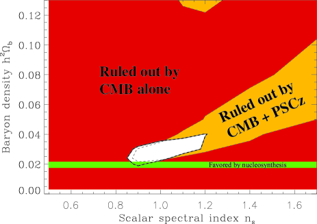
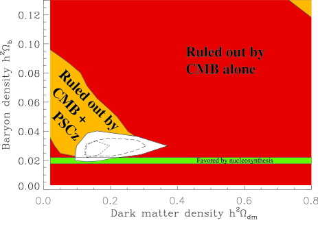
The nucleosynthesis prior has a greater influence because it does not agree all that well with what the CMB+LSS data prefer. Although adding PSCz is seen to pull down the preferred baryon density slightly, reducing the 95% lower limit from 0.024 (CMB only) to 0.020 (CMB+PSCz), the preferred value of 0.028 still exceeds the BBN value. It is well-known that CMB likes either a high baryon density or a red-tilt $n<1$ because of the low second acoustic peak [1, 2, 3, 4, 39, 40], and the CMB exclusion region to the lower right in Figure 7 illustrates this tradeoff. Enforcing the BBN baryon value therefore shifts the preferred tilt-range away from the scale-invariant $n_{s}\sim 1$ case to $n_{s}\sim 0.9$. Since $\omega_{\rm b}$ is one of the few parameters affecting the relative heights of the acoustic peaks (together with $\omega_{\rm dm}$, $n_{s}$ and, marginally, $f_{\nu}$), eliminating the uncertainty in $\omega_{\rm b}$ with the BBN prior also tightens the constraints on these other parameters. In particular, the link between $\omega_{\rm b}$ and $\omega_{\rm dm}$ is illustrated in Figure 8.

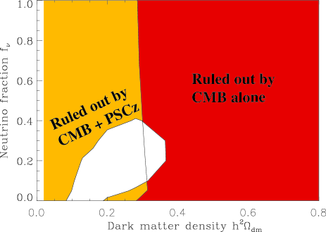
We found one additional prior that had a non-negligible effect: that on neutrinos. As illustrated in Figure 9, inclusion of neutrinos substantially weakens the upper limits on the dark matter density. Since the neutrino fraction $f_{\nu}$ has only a weak effect on the CMB, this effect clearly comes from LSS. A larger dark matter density $\omega_{\rm dm}$ pushes matter-radiation equality back to an earlier time, shifting the corresponding turnover in $P(k)$ to the right and thereby increasing the ratio of small-scale to large-scale power. Increasing the neutrino fraction counteracts this by suppressing the small-scale power (without affecting the CMB much), thereby weakening the upper limit on $\omega_{\rm dm}$. Imposing the prior $f_{\nu}=0$ alone, without nucleosynthesis or Hubble priors, tightens the CMB+PSCz constraint $\omega_{\rm dm}<0.32$ from Table 1 to $\omega_{\rm dm}<0.19$.

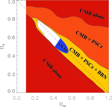
Since the constraints on $\omega_{\rm dm}$ are tightened by fixing both $\omega_{\rm b}$ (Figure 8) and $f_{\nu}$ (Figure 9), the “concordance” case in Table 1 gives quite tight constraints on the dark matter density. The $h$ prior helps turn this $\omega_{\rm dm}$ constraint into a measurement of $\Omega_{\rm dm}$, and the measurement $\Omega_{\rm k}\sim 0$ therefore gives an indirect constraint on the cosmological constant via $\Omega_{\Lambda}=1-\Omega_{\rm k}-\Omega_{\rm dm}-\Omega_{\rm b}$. This is illustrated in Figure 6, where the concordance constraints close off the allowed region by placing a lower limit on $\Omega_{\Lambda}$. This lower limit on $\Omega_{\Lambda}$ goes away if we drop either the $\omega_{\rm b}$-prior or the $f_{\nu}$-prior.

FIG. 6.: Constraints in the $(\Omega_{\rm m},\Omega_{\Lambda})$-plane. The shaded regions are ruled out at 95% confidence by the information indicated. The allowed (white) region is seen to be centered around flat models, which fall on the dashed line.

FIG. 7.: Constraints in the $(n_{s},\omega_{\rm b})$-plane. Note that PSCz not only shrinks the allowed region (white), but also pushes it slightly down to the left (the dashed line indicates the CMB-only boundary).

FIG. 8.: Constraints in the $(\omega_{\rm dm},\omega_{\rm b})$-plane. As in the previous figure, adding PSCz prohibits high baryon solutions and allows slightly lower $\omega_{\rm b}$-values than CMB alone. The dashed curve within the allowed (white) region show the sharper constraint obtained when imposing the priors for a flat, scalar scale-invariant model ($\Omega_{\rm k}=r=0$, $n_{s}=1$). The dotted curve shows the effect of requiring negligible neutrino density ($f_{\nu}\sim 0$) in addition.

FIG. 9.: Constraints in the $(\omega_{\rm dm},f_{\nu})$-plane. The shape of the allowed (white) region explains why the prior $f_{\nu}=0$ tightens the upper limit on the dark matter density. The vertical line shows the CMB-only boundary before PSCz is added.

C Constraints on other parameters

1 Hubble parameter

Table 1 shows that the constraints on the Hubble parameter $h$ are quite weak for the CMB+LSS case. However, the bound $h<0.78$ (95%) for the concordance case is noteworthy since it is much stronger than (and hence independent of) the prior $h=0.74\pm 0.08$ that was used.

2 Ionization redshift

In the approximation that the diffuse hydrogen in the Universe became fully ionized rather abruptly at a redshift $z_{ion}$, this quantity is well approximated by (e.g., Peebles 1993)

$$z_{ion}=8.9\>\left({\tau h\over\omega_{\rm b}}\right)^{2/3}\Omega_{\rm m}^{1/3}$$ (2)

as long as $z_{ion}\gg 1$. Although the constraints in Table 1 agree well with what is predicted in recent simulations, more extreme models are seen to be ruled out. Earlier CMB constraints on $z_{ion}$ were studied in [42, 43].

3 Age of Universe

The ability to place constraints in the $(\Omega_{\rm m},\Omega_{\Lambda})$-plane is allowing the age of the Universe to be predicted with improved accuracy [44, 5]. The 95% confidence interval for our concordance case, 12.1–14.6 Gigayears, is consistent with direct age determinations from, e.g., globular clusters [45, 46].

IV DISCUSSION

We have presented a method for rapid and accurate power spectrum calculation for large numbers of CMB models and used it to constrain jointly 11 cosmological parameters from current CMB and galaxy clustering data. Perhaps the most interesting results of this paper are the numbers themselves, listed in the CMB+LSS columns of Table 1, and their striking robustness to imposing various priors. A superficial glance at the constraint figures might suggest that little has changed since the first analysis of Boomerang + Maxima [2], or even since the pre-Boomerang analysis of [32], since the plots look rather similar. However, whereas these earlier papers obtained strong constraints only with various poorly justified priors such as no tensors, no tilt or no curvature, the joint CMB + LSS data are now powerful enough to speak for themselves, without needing any such prior props.

A New public software

Our new power spectrum calculation method accelerates CMBfast by about a factor $10^{3}$. It is accurate to about 1–2% for $C_{\l}$ on all angular scales and to about 1% for $P(k)$ on scales $k<0.15\,h\,{\rm Mpc}^{-1}$. Since this is roughly the intrinsic accuracy level of CMBfast itself, there is no reason not to take advantage of this technique when constraining cosmological parameters. A modified version of CMBfast incorporating our $k$-split method will be made publicly available at www.sns.ias.edu/$\sim$matiasz/CMBFAST/cmbfast.html.

B Caveats

Let us now discuss assumptions and approximations that underly our analysis.

For both the CMB and LSS likelihood calculations, the percent level inaccuracies in our power spectrum computation are likely to have a negligible effect. Indeed, the least accurate models tend to be wild ones that are inconsistent with the data in any case. On the LSS side, the dominant uncertainties are likely to be related to the measured $P(k)$ instead. Specifically, our use of the measurements of the PSCz real-space power [20] assumed both that linear perturbation theory was valid and that the bias was scale-independent on these scales. Let us now discuss both of these assumptions in turn.

To assess the possibility that nonlinear effects at $k\sim 0.1$–$0.3\,h\,{\rm Mpc}^{-1}$ had tainted our results, we repeated the entire analysis twice, discarding all $P(k)$-measurements for $k$ exceeding $0.2\,h\,{\rm Mpc}^{-1}$ and $0.1\,h\,{\rm Mpc}^{-1}$, respectively. The upper limit $f_{\nu}<0.38$ on the neutrino fraction was weakened for the 0.2 case and went away completely for the 0.1 case. Thus the upper limit on neutrinos is sensitive to information at mildly nonlinear scales. The upper limit on $n_{s}$ was also weakened as the lever arm shortened, but only very slightly, from $n_{s}<1.16$ at $0.3\,h\,{\rm Mpc}^{-1}$ to $n_{s}<1.18$ and $n_{s}<1.19$ at $0.2$ and $0.1\,h\,{\rm Mpc}^{-1}$, respectively. Other constraints were less affected.

The redshift distortion study reported in [20] suggested that, while nonlinear effects are visible in the galaxy-velocity power spectrum already at scales $k\approx 0.15\,h\,{\rm Mpc}^{-1}$, linear theory is probably a fair approximation down to $k\approx 0.3\,h\,{\rm Mpc}^{-1}$. A subsequent study [47] of the nonlinear power spectrum of PSCz has shown that the galaxy power spectrum is likely to be antibiased relative to the matter power spectrum at translinear scales, a conclusion previously arrived at by [28, 48]. Such antibias tends to cancel the effects of nonlinearity in the matter power spectrum, making the galaxy power spectrum appear similar to the linear matter power spectrum down to $k\approx 0.3\,h\,{\rm Mpc}^{-1}$. The fact that the relative bias between APM and PSCz galaxies is consistent with being constant, $b_{\rm APM}/b_{\rm PSCz}\approx 1.15$, for $k\leq 0.3\,h\,{\rm Mpc}^{-1}$ [49, 47] adds further circumstantial evidence suggesting that the galaxy power spectra are near linear at these scales.

We therefore conclude that including the PSCz data at $k=0.1$–$0.3\,h\,{\rm Mpc}^{-1}$ does not bias the results significantly, and that, aside from the constraint on neutrinos, the information from PSCz is not dominated by these last few bins.

Although most theoretical work has suggested that the bias $b$ is unlikely to vary much on linear scales, we must still be open to the possibility of scale-dependent bias masquerading as a cosmological effect. For instance, one might imagine that more luminous galaxies are more highly biased, and that they carry a greater statistical weight for the leftmost $k$-bands since they remain in the magnitude-limited 0.6 Jy sample even at great distances. Such a luminosity bias could masquerade as a slight red-tilt $n_{s}<1$. However, three recent studies [50, 51, 52] all conclude that PSCz galaxies of different luminosity cluster similarly.

On the CMB side, a long list of approximations in our treatment were discussed in [32], involving both the likelihood calculation [53] and the marginalization. The dominant limitation is likely to be that we have not included the full window functions and slight band-band correlations of Boomerang and Maxima, but this is unfortunately not possible until the relevant Fisher matrices are made public by the two experimental teams.

Positive correlations between neighboring data points makes is easier (in terms of chi-squared cost) to shift the overall height of say the first peak up and down, thereby weakening the constraints on parameters that are measured mainly from peak heights ($\omega_{\rm b}$, $\omega_{\rm cdm}$, $n_{s}$). This effect is similar to that of calibration errors, which we did include. The fact that our best fit models tend to predict a lower first peak than much of the data illustrates the effect of calibration errors and also shows that an extremely high first peak is hard to achieve given the other constraints.

The extraction of constraints on individual parameters from the multidimensional likelihood function can be done in a number of different ways. Three ways of marginalizing are discussed in [32] (by integration, by maximization over the grid and by maximization over a smooth interpolating function), all of which have been used in the recent literature. An encouraging indication that our results are insensitive to the method of marginalization comes from comparing the marginalized constraints from Table 1 with those obtained without any marginalization, from the above-mentioned computation of means and standard deviations by summing over the grid. These completely different methods give quite similar results for all well-constrained parameters. A typical example is the $2\sigma$ range for $\omega_{\rm dm}$ for the “concordance” case, coming out as $0.110<\omega_{\rm dm}<0.170$ (marginalized) and $0.105<\omega_{\rm dm}<0.172$ (from moments). Even for $\tau$, the parameter with the most non-Gaussian likelihood, the $2\sigma$ “concordance” upper limits are similar: 0.161 and 0.163, respectively.

Finally, although we repeatedly referred to the “no prior” case for our CMB + LSS analysis, it is important to bear in mind that there is strictly speaking no such thing as no priors. Specifically, all our calculations assumed that the adiabatic inflationary paradigm is correct. We also assumed that the dark energy was a cosmological constant rather than some form of “quintessence” with a different equation of state. Finally, the edges of our parameter grid imposed a hard-wired top hat prior. This had a negligible effect on our results for all parameters except one, since the likelihood dropped to negligible values well before reaching the boundary of our 11-dimensional parameter space. The one exception involved $\Omega_{\Lambda}$, since Figure 6 illustrates that negative $\Omega_{\Lambda}$ cannot be excluded except when either BBN or SN 1a information is included.

C Comparison with other recent work

Our results agree fairly well with the recent constraints from other groups [1, 3, 4, 5, 6]. The analysis most comparable to ours is that of Jaffe et al. [5]. That study limits LSS-information to that incorporated in a shape parameter and a normalization parameter, and uses a smaller CMB data set, limiting the analysis to COBE, Boomerang and Maxima. The main effect of this culling is likely to enter on scales $50\mathrel{\hbox to0.0pt{\lower 3.0pt\hbox{$\mathchar 536\relax$}\hss}\raise 2.0pt\hbox{$\mathchar 316\relax$}}\l\mathrel{\hbox to0.0pt{\lower 3.0pt\hbox{$\mathchar 536\relax$}\hss}\raise 2.0pt\hbox{$\mathchar 316\relax$}}200$, covering the rise toward the first acoustic peaks, where Boomerang and Maxima are both sample variance limited and other experiments have covered a substantially larger sky area. In addition, [5] limit their parameter space to no neutrinos and no tensors ($f_{\nu}=r=0$), employ a different numerical marginalization scheme and include the above-mentioned proprietary band correlations. The fact that our results agree so well despite all these technical differences is quite reassuring, indicating that the data are now good enough to make the results insensitive to details of method. The stronger upper CMB+LSS limit on $\omega_{\rm dm}$ obtained in [5], which indirectly gives $\Omega_{\Lambda}\mathrel{\hbox to0.0pt{\lower 3.0pt\hbox{$\mathchar 536\relax$}\hss}\raise 2.0pt\hbox{$\mathchar 318\relax$}}0.5$ as described above, is presumably due to their no-neutrino prior $f_{\nu}=0$, as can be understood from Figure 9. The fact that their CMB-only constraints are stronger than ours traces back to their no-tensor $r=0$ prior — this prior eliminates the $n_{s}-r-\omega_{\rm b}$ degeneracy that we needed the full PSCz data to break, and automatically excludes models such as the one shown in Figure 1.

Our results also agree well with those from the likelihood analysis of Kinney et al. [6]. Although this analysis has $f_{\nu}=0$, a prior for $n_{t}$ and a limited $\tau$-range, it includes a thorough treatment of tensor modes and maps out the $(n_{s},r)$-plane in detail. The study finds that quite blue-tilted models are allowed when $r$ is large, precisely the effect that degrades our CMB-only constraints — see also [54, 55].

D Towards a refined concordance model

It is well-known that different types of measurements can complement each other by breaking degeneracies. However, even more importantly, multiple data sets allow numerous consistency checks to be made. The present results allow a number of such tests.

1 Baryons

Perhaps the most obvious one involves the baryon fraction. Although there is still some tension between BBN (preferring $\omega_{\rm b}\sim 0.02$ and CMB+LSS (preferring $\omega_{\rm b}\sim 0.03$), an issue which will undoubtedly be clarified by improved data within a year, the most striking point is that the methods agree as well as they do. That one method involving nuclear physics when the Universe was minutes old and another involving plasma physics more than 100,000 years later give roughly consistent answers, despite involving completely different systematics, can hardly be described as anything short of a triumph for the Big Bang model.

It is noteworthy that our addition of LSS information pulls down the baryon value slightly, so that a BBN-compatible value $\omega_{\rm b}=0.02$ is now within the 95% confidence interval. Part of the reason that that the CMB alone gave a stronger lower limit may be a reflection of the Bayesian likelihood procedure employed in this and all other recent papers on the topic: when a large space of high $\omega_{\rm b}$-values are allowed, the relative likelihood for lower values drops.

In all three cases listed in Table 1, the best fit model is consistent with the data in the sense of giving an acceptable $\chi^{2}$-value. The “CMB only” case gives $\chi^{2}\approx 70.3$ for 87 degrees of freedom. The “CMB+PSCz” case gives $\chi^{2}\approx 88.7$, which rises to 95.6 for the “concordance” case — all for $\approx 109-11$ degrees of freedom. The effective number of degrees of freedom might be a few larger than this, since some of the 11 parameters had little effect, but even taking this into account, all fits are good in the sense of giving reduced $\chi^{2}$-values of order unity.

Apart from BBN, our baryon value also agrees with the range $0.007\mathrel{\hbox to0.0pt{\lower 3.0pt\hbox{$\mathchar 536\relax$}\hss}\raise 2.0pt\hbox{$\mathchar 316\relax$}}\Omega_{\rm b}\mathrel{\hbox to0.0pt{\lower 3.0pt\hbox{$\mathchar 536\relax$}\hss}\raise 2.0pt\hbox{$\mathchar 316\relax$}}0.041$ inferred from a low-redshift inventory [67] and the range $0.015\mathrel{\hbox to0.0pt{\lower 3.0pt\hbox{$\mathchar 536\relax$}\hss}\raise 2.0pt\hbox{$\mathchar 316\relax$}}\omega_{\rm b}\mathrel{\hbox to0.0pt{\lower 3.0pt\hbox{$\mathchar 536\relax$}\hss}\raise 2.0pt\hbox{$\mathchar 316\relax$}}0.03$ at redshifts of a few from the Ly$\alpha$ forest [68, 69, 70, 71]. The inferred baryon fraction $\omega_{\rm b}/\omega_{\rm dm}\sim 15\%$ agrees well with that inferred from galaxy clusters [72, 73] for reasonable $h$-values.

It is difficult to contemplate the PSCz data in Figure 2 without wondering whether they show evidence for baryonic wiggles in the matter power spectrum. Intriguingly, the location and amplitude of the wiggles in the PSCz power spectrum fit well to a flat, pure baryon model with $\Omega_{\Lambda}=.86$ and $\Omega_{\rm m}=\Omega_{\rm b}=0.14$ (for $h=0.7$), albeit with a large blue tilt, $n_{s}=2$, but agrees poorly with the CMB. The PSCz data are also entirely consistent with a wiggle-free spectrum.

2 Dark energy

Another important cross-check involves the cosmological constant. Although the constraint $0.49<\Omega_{\Lambda}<0.74$ from Table 1 does not involve any supernova information, it agrees nicely with the recent accelerating universe predictions from SN 1a [74, 75]. This agreement is illustrated in Figure 6, which shows the SN 1a constraints from [76] combining the data from both teams. As frequently pointed out, the conclusion $\Omega_{\rm m}\sim 0.35$ also agrees well with a number of other observations, e.g., the cluster abundance at various redshifts [77, 78, 79, 72] and cosmic velocity fields [80], although there is still some internal controversy in these two areas (see, e.g., [81]).

FIG. 10.: The upper panel shows $\chi^{2}$ for the linear redshift distortion parameter beta measured from the PSCz data. Specifically, $\chi^{2}$ was computed using the galaxy-galaxy, galaxy-velocity and velocity-velocity power spectra but no CMB information, then minimized over all parameters except $\Omega_{\rm k}$ and $\Omega_{\Lambda}$. The fact that the resulting $\chi^{2}(\Omega_{\rm k},\Omega_{\Lambda})$ falls near a 1-dimensional curve with little scatter shows that it essentially only depends on one particular function of these two parameters, the linear growth rate $f(\Omega_{\rm m},\Omega_{\Lambda})$ (equivalently the redshift distortion parameter $\beta=f/b$). The best fit curve (thick line) has a slower rise for high $\beta$ than a parabola (thin line). The lower panel shows the corresponding likelihood $\L\propto e^{-\chi^{2}/2}$, and the $1\sigma$ and $2\sigma$ confidence limits are where this (thick) curve crosses the dashed lines.

3 Bias

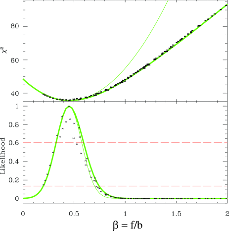
A third cross-check is more subtle but equally striking, involving the bias of the PSCz galaxies — we can measure it in two completely independent ways. One is by comparing the amplitude of the CMB and galaxy power spectra, which gives the constraints listed in Table 1. The other way is via the linear redshift space distortion parameter $\beta=f(\Omega_{\rm m},\Omega_{\Lambda})/b$, where $f(\Omega_{\rm m},\Omega_{\Lambda})\approx\Omega_{\rm m}^{0.6}$ is the dimensionless linear growth rate [82, 83, 84]. We therefore remove the CMB data (which eliminates the $\beta$-constraints from Table 1) and add in their place the two PSCz power spectra from [20] that we discarded above. These are the galaxy-velocity and velocity-velocity power spectra from the stochastic bias formalism, roughly speaking corresponding to the quadrupole and hexadecapole of the redshift space distortions. The redshift distortion parameter for the PSCz galaxies was measured to be $\beta=0.41^{+.13}_{-.12}$ [20], a result in good agreement with the PSCz team’s own most recent measurement, $\beta=0.39\pm 0.12$ [85]. Both of these measurements involved a limited marginalization over the power spectrum. Here we marginalize the full likelihood function over all our cosmological parameters except $\beta$. As can be seen in Figure 10, this gives the $1\sigma$ measurement $\beta=0.45^{+.14}_{-.12}$. The fact that this agrees so well with the corresponding $1\sigma$ measurement $\beta=0.51\pm 0.08$ from Table 1 for the concordance case means that a highly non-trivial consistency test has been passed.

E Concordance

In conclusion, the simple “concordance” model in the last columns of Table 1 (plotted in Figure 3) is at least marginally consistent with all basic cosmological constraints, including CMB, PSCz and nucleosynthesis. Specifically, as discussed above, our calculations show that it has passed three non-trivial consistency tests. Moreover our concordance model is encouragingly robust towards imposing a score of prior constraints in various combinations. Cosmology seems to be on the right track!

The authors wish to thank Angélica de Oliveira-Costa, Daniel Fisher, Brad Gibson, Wayne Hu, William Kinney, Arthur Kosowsky, and Nikhil Padmanabhan for useful discussions and helpful comments. Support for this work was provided by NSF grant AST00-71213, NASA grants NAG5-7128 and NAG5-9194, the University of Pennsylvania Research Foundation, and Hubble Fellowship HF-01116.01-98A from STScI, operated by AURA, Inc. under NASA contract NAS5-26555.

A BASIC METHOD IMPROVEMENTS

As mentioned, our method is based on the one described in [32], but with a number of extensions and improvements as detailed below. It consists of the following steps:

• Compute power spectra $C_{\l}$ and $P(k)$ for a grid of models in our 11-dimensional parameter space.

• Compute a likelihood for each model that quantifies how well it fits the data.

• Perform 11-dimensional interpolation and marginalize to obtain constraints on individual parameters and parameter pairs.

Our main improvement over [32] is in step 1. We improve the technique for accelerated CMB power spectrum calculation so that it becomes essentially as accurate as CMBfast itself, simply about $10^{3}$ times faster. We also add a simple but accurate technique to compute the grid of matter power spectra rapidly.

1 Improved choice of parameters

Reference [32] explored the 10-dimensional parameter space involving the reionization optical depth $\tau$, the primordial amplitudes $A_{s}$, $A_{t}$ and tilts $n_{s}$, $n_{t}$ of scalar and tensor fluctuations, and various contributions $\Omega_{i}$ to critical density. The $\Omega_{i}$ included were for curvature $\Omega_{\rm k}$, vacuum energy $\Omega_{\Lambda}$, cold dark matter $\Omega_{\rm cdm}$, hot dark matter (neutrinos) $\Omega_{\nu}$ and baryons $\Omega_{\rm b}$. Since it is computationally advantageous to work with parameters that are closely linked to the most important physical processes involved, reference [32] used the parameter vector

$${\bf p}\equiv(\tau,\Omega_{\rm k},\Omega_{\Lambda},\omega_{\rm cdm},\omega_{\rm b},\omega_{\nu},n_{s},n_{t},A_{s},A_{t}),$$ (A1)

where the physical densities $\omega_{i}\equiv h^{2}\Omega_{i}$.

Unless $\Omega_{\nu}\ll 1$, the neutrinos left over from the early Universe were heavy enough to be fairly non-relativistic during the processes that created the acoustic peaks, and thereby had almost the same effect as cold dark matter on the CMB. The CMB power spectrum therefore depends mainly on the total nonbaryonic (cold$+$hot) dark matter density $\omega_{\rm dm}\equiv\omega_{\rm cdm}+\omega_{\nu}$ and only quite weakly on the hot fraction $f_{\nu}\equiv\omega_{\nu}/\omega_{\rm dm}$. We therefore replace our old parameters $(\omega_{\rm cdm},\omega_{\nu})$ by $(\omega_{\rm dm},f_{\nu})$. This allows us to accurately compute the weak $f_{\nu}$-dependence of the scalar CMB power spectrum by using a coarse grid $f_{\nu}=$0.0, 0.3, 1.0 and interpolating. Moreover, the tensor fluctuations are essentially independent of $f_{\nu}$, so we only compute them for $f_{\nu}=0$.

In this paper, we need to add one more parameter, relating the theoretically predicted power spectrum of matter $P(k)$ to that of PSCz galaxies $P_{g}(k)$ on large scales. This parameter is the bias $b\equiv[P_{g}(k)/P(k)]^{1/2}$ from the stochastic bias formalism [86, 87, 88]. Although it can in principle depend on scale, we will assume that it is constant on the large scales that we consider [24, 25, 26, 27, 28, 29, 30, 31]. We will make no assumptions about the value of $b$, however, and therefore marginalize over this parameter before quoting constraints on the other ten. In summary, we use the parameter vector

$${\bf p}\equiv(\tau,\Omega_{\rm k},\Omega_{\Lambda},\omega_{\rm dm},\omega_{\rm b},f_{\nu},n_{s},n_{t},A_{s},A_{t},b).$$ (A2)

Note that the Hubble constant is not a twelfth independent parameter, since

$$h=\sqrt{\omega_{\rm dm}+\omega_{\rm b}\over 1-\Omega_{\rm k}-\Omega_{\Lambda}}.$$ (A3)

We wish to probe a large enough region of parameter space to cover even quite unconventional models. This way, constraints from non-CMB observations can be optionally included by explicitly multiplying the likelihood function $\L({\bf p})$ by a Bayesian prior rather than being hard-wired in from the outset. To avoid dealing with prohibitively many models, we use a roughly logarithmic grid spacing for $\omega_{\rm m}$, $\omega_{\rm b}$ and $\omega_{\nu}$, a linear grid spacing for $\Omega_{\rm k}$ and $\Omega_{\Lambda}$, a hybrid for $\tau$, $f_{\nu}$, $n_{s}$ and $n_{t}$, and (as described below) a continuous grid for $A_{s}$, $A_{t}$ and b.

The recent progress in CMB accuracy has been so dramatic that the grids used in some recent papers [2, 3] are already almost too sparse to accurately sample the small allowed regions of parameter space. We therefore modify the grid from [2] to zoom in on the favored parameter ranges while still retaining some outlier points to be on the safe side. We let the parameters take on the following values:

• $\tau=0,0.05,0.1,0.2,0.3,0.5,0.8$

• $\Omega_{\Lambda}=0,0.1,....,1.0$

• $\Omega_{\rm k}$ such that $\Omega_{\rm m}\equiv 1-\Omega_{\rm k}-\Omega_{\Lambda}=0.1,0.2,...,1.0$

• $\omega_{\rm dm}=.02,.05,.08,.13,.16,.20,.28,.40,.80$

• $\omega_{\rm b}=.003,.013,.016,.020,.024,.03,.04,.05,.08,.13$

• $f_{\nu}=0,0.05,0.1,0.2,0.3,0.4,0.6,0.8,1.0$

• $n_{s}=0.5,0.7,0.8,0.9,1.0,1.1,1.2,1.4,1.7$

• $n_{t}=-1.00,-0.70,-0.40,-0.20,-0.10,0$

• $A_{s}$ is not discretized

• $A_{t}$ is not discretized

• $b$ is not discretized

Note that the extent of the $\Omega_{\rm k}$-grid depends on $\Omega_{\Lambda}$, giving a total of $10\times 11=110$ points in the $(\Omega_{\rm m},\Omega_{\Lambda})$-plane. Our discrete grid thus contains $7\times 110\times 9\times 10\times 9\times 9\times 6=33,679,800$ models. As in [32], the main limitation on this grid size is disk space rather than CPU time.

2 The three basic spectra and their normalization

It is convenient to write the two power spectra $C_{\ell}$ and $P_{g}(k)$ that we can measure as

$$C_{\ell} = A_{s}C_{\ell}^{\rm scalar}+A_{t}C_{\ell}^{\rm tensor},$$ (A4)

$$P_{g}(k) = A_{s}b^{2}P(k),$$ (A5)

where the three basic power spectra $C_{\ell}^{\rm scalar}$, $C_{\ell}^{\rm tensor}$ and $P(k)$ are all normalized consistently, corresponding to a fixed amplitude of the gravitational potential $\psi$ when each mode is outside horizon. The default output of CMBfast first normalizes the CMB output to COBE, but the new version allows output of the raw unnormalized spectra that we need. $C_{\ell}^{\rm scalar}$ depends on $(\tau,\Omega_{\rm k},\Omega_{\Lambda},\omega_{\rm dm},\omega_{\rm b},f_{\nu},n_{s})$, $C_{\ell}^{\rm tensor}$ depends on $(\tau,\Omega_{\rm k},\Omega_{\Lambda},\omega_{\rm dm},\omega_{\rm b},n_{t})$ and $P(k)$ depends on $(\Omega_{\rm k},\Omega_{\Lambda},\omega_{\rm dm},\omega_{\rm b},f_{\nu},n_{s})$, so we need to compute three separate grids of models of dimensionality 7, 6 and 6, respectively. We describe a fast and accurate way of doing this in Appendices B and C.

3 Likelihoods and marginalization

We compute the CMB likelihood exactly as in [32], i.e., using the first results from Maxima and Boomerang as well as all prior experiments [89] (shown in Figure 1) and taking into account the effect of calibration errors.

For the PSCz galaxy power spectrum, we use only the band power measurements plotted in black in Figure 2, omitting the ones further to the right. This is a subset of the measurements from [20] that includes information only at scales $k<0.3\,h\,{\rm Mpc}^{-1}$ to ensure that we stay clear of nonlinear effects. As a further precaution, we examine how the results change when this cut is further sharpened in Section IV B. We approximate the corresponding likelihood function by the multivariate Gaussian $\L_{\rm lss}\propto e^{-{1\over 2}\chi^{2}}$, where $\chi^{2}$ is computed using the measurements in Figure 2. Each point in Figure 2 represents an uncorrelated measurement of the power in a well-defined band whose FWHM is indicated by the horizontal bar. In computing the likelihood, we take into account the detailed form of each band-power window.

The joint likelihood function is obtained by multiplying the CMB and LSS likelihoods. Throughout this paper we marginalize over the amplitudes $A_{s}$, $A_{t}$, and the bias factor $b$. Equations (A4) and (A5) show that we can equivalently marginalize over these parameters separately for the CMB and LSS likelihoods before multiplying them together, which simplifies the calculations in practice.

B METHOD FOR COMPUTING $C_{\l}$

We compute $C_{\ell}^{\rm tensor}$ as described in [32]: by running CMBfast merely for a coarser grid in $\omega_{\rm dm}$ and $\omega_{\rm b}$ (on which the dependence is weak) and interpolating onto our full grid using a regularized multidimensional spline. Since $C_{\ell}^{\rm tensor}$ only contributes to the first few hundred multipoles, it is much faster to compute than $C_{\ell}^{\rm scalar}$, which is the real challenge.

1 The $k$-space split

The idea introduced in [55] and [32] was roughly speaking to compute the $\l\mathrel{\hbox to0.0pt{\lower 3.0pt\hbox{$\mathchar 536\relax$}\hss}\raise 2.0pt\hbox{$\mathchar 316\relax$}}100$ and $\l\mathrel{\hbox to0.0pt{\lower 3.0pt\hbox{$\mathchar 536\relax$}\hss}\raise 2.0pt\hbox{$\mathchar 318\relax$}}100$ parts of $C_{\ell}^{\rm scalar}$ separately and splice them together afterwards. The former can be computed just as fast as $C_{\ell}^{\rm tensor}$, since its dependence on $\omega_{\rm dm}$ and $\omega_{\rm b}$ is weak and it is essentially independent of $f_{\nu}$. The latter can be computed rapidly as well, since the only effect of $\Omega_{\rm k}$ and $\Omega_{\Lambda}$ is to shift it sideways in a known way. To a decent approximation, the $\tau$-dependence can be incorporated analytically as well, as simply a multiplication by $e^{-2\tau}$. However, since there is a small bump of regenerated power from the new last scattering surface (which moves to larger $\l$ as $\tau$ is increased), we opt to include $\tau$ explicitly this time — as mentioned, the algorithm is so fast that we are limited by disk space rather than CPU time anyway. In short, the high-$\l$ part of $C_{\ell}^{\rm scalar}$ only needs to be computed on a 5-dimensional grid spanned by $(\tau,\omega_{\rm dm},\omega_{\rm b},f_{\nu},n_{s})$. Moreover, this is really only 4 “hard” parameters, since CMBfast treats multiple $n_{s}$-values simultaneously with no slowdown.

Although this approximation works well, it is typically only accurate to 5–10% or so. The main problem is with the splicing itself, since projection effects alias power from a given physical scale to quite a broad range of $\l$-values, blurring the separation between the low and high grids. The new method that we present here bypasses this problem by making the split directly in $k$-space, where the actual physics takes place. Specifically, we modify CMBfast to save only the contribution to $C_{\ell}$ from below or above a certain wave number $k_{*}$ when it integrates the Boltzmann equation.

The “low” $(k<k_{*})$ contribution corresponds to fluctuations on scales outside the horizon at recombination. This makes it almost independent of the causal microphysics that creates the familiar acoustic peaks, i.e., almost independent of $\omega_{\rm dm}$, $\omega_{\rm b}$ and $f_{\nu}$. Rather, it is dominated by what happens at low redshift (the late integrated Sachs-Wolfe effect, reionization, etc.).

In contrast, the “high” $(k>k_{*})$ contribution is essentially unaffected by low redshift effects, so $\Omega_{\rm k}$ and $\Omega_{\Lambda}$ (or some other dark energy component that was negligible at $z\mathrel{\hbox to0.0pt{\lower 3.0pt\hbox{$\mathchar 536\relax$}\hss}\raise 2.0pt\hbox{$\mathchar 318\relax$}}10^{3}$) will merely take the pattern put in place at $z\sim 10^{3}$ and shift it sideways according to the angle-distance relationship. Suppressing the other 9 parameters, we thus have

$$C_{\ell}^{\rm scalar}(\Omega_{\rm k},\Omega_{\Lambda})\approx C_{\ell}^{\rm low}(\Omega_{\rm k},\Omega_{\Lambda})+C_{\l^{\prime}}^{\rm high}(0,0),$$ (B1)

where $\l^{\prime}\equiv[d_{\rm lss}(\Omega_{\rm k},\Omega_{\Lambda})/d_{\rm lss}(0,0)]\l$ and $d_{\rm lss}$ is the angular diameter distance to the last scattering surface in ${\rm Mpc}$ (not in $h^{-1}{\rm Mpc}$).

We tune the choice of $k_{*}$ differently for each model, choosing $k_{*}=1.5/d_{\rm shor}$ where $d_{\rm shor}=\int c_{s}d\eta$ is the sound horizon at decoupling (here $c_{s}$ is the sound speed and $\eta$ denotes conformal time). In $\l$-space, this value of $k_{*}$ corresponds approximately to the place were we did the splitting in [32], i.e., to the early rise of the first acoustic peak ($\l=100$ for flat models, higher/lower $\l$ for open/closed models).

FIG. 11.: Three examples of our method for computing CMB power spectra. The three panels show a flat $\Lambda$-model ($\Omega_{k}=0,\Omega_{\Lambda}=0.7$ — top), a moderately open model ($\Omega_{k}=0.4,\Omega_{\Lambda}=0.3$ — middle) and a moderately closed model ($\Omega_{k}=-0.2,\Omega_{\Lambda}=0.9$ — bottom). All three models have $\omega_{dm}=0.1225$, $\omega_{b}=0.0245$ and $f_{\nu}=0$. The model $C_{\ell}^{\rm high}$ used in the $k>k_{*}$ calculation had $\Omega_{k}=\Omega_{\Lambda}=0$, and is simply shifted sideways differently in each panel, whereas the $(k<k_{*})$ spectra $(C_{\ell}^{\rm low})$ were computed separately for each model. The solid line shows the full CMBfast calculation while the long dashed line shows the result of our new method, i.e., the sum of the two dashed curves.

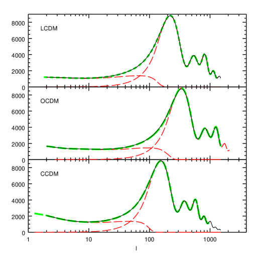
Figure 11 shows an example of this splitting technique. We show three panels with a flat $\Lambda$ model, a moderately open model and a moderately closed models. Each panel has four curves. The solid line is the model calculated fully with CMBfast from scratch. The long dashed line shows the same model calculated with our new technique, and is seen to differ by less than $2\%$ across the spectrum. For completeness we also show the spectra for $k<k_{*}$ and $k>k_{*}$ that were added in each panel. Note that the $k>k_{*}$ curve is the same for the three panels, merely shifted sideways by different amounts to match the angular diameter distance.

We do not make a sharp cut at $k_{*}$. Rather, to avoid numerical problems, we use a soft cut defined by the function

$$w(k)\equiv{2\over 1+e^{2\left(k\over k_{*}\right)^{4}}},$$ (B2)

Specifically, when computing $C_{\ell}^{\rm low}$ and $C_{\ell}^{\rm high}$, we multiply the primordial $k$ power spectrum by $w(k)$ and $[1-w(k)]$, respectively. Note that even a sharp $k$-cut would result in a fuzzy $\l$-cut, since projection effects alias a given $k$-value onto a range of $\l$-values.

2 Testing the $C_{\ell}$ accuracy

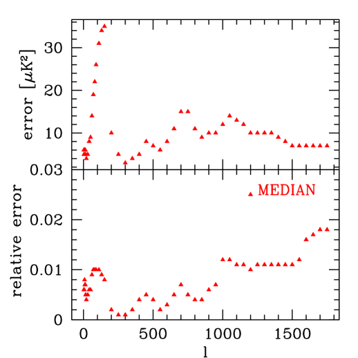
To test the accuracy of our method, we drew a random sample of $\sim 10^{3}$ of the models from our final grid and recomputed them from scratch with CMBfast. We also added about $10^{2}$ models to the test sample by hand that we suspected might be particularly troublesome. The results are shown in Figure 12. As can be seen, the median accuracy is better than $2\%$ for most $\l$-values. It should be noted that this is a test not only of the $k$-space splitting technique, but of our full pipeline, which includes several steps of interpolation.

One interesting thing to point out is that our median error is substantially lower than our mean error. This occurs because there are a small number of outlier models where we find significantly larger errors. We should first note that our worst model is never more that $30\%$ off for $\l<1000$. An examination of the worst models reveals our main sources of inaccuracies. Our main source is percent level errors is the calculation of the angular diameter distances, which lead to a small relative shift between the spectra. In models with sharp peaks, this can lead to large relative errors although the two curves are very similar to each other. Thus this is quite a benign error that can be further improved by a better calculation of the angular diameter distance but that has no effect for the likelihood of current data which has window functions that are much wider than this small shift.

The second source of error is in the region were we combine the high and low $k$ spectra. Usually our worst models (which are off by less that $15\%$ in this region) have a significant ISW contribution at low $\l$, so that this ISW contribution is still significant for the high $k$ wavelengths but were not included because we always shift flat $\Omega_{m}=1$ models. Although this source of error is inherent to our method, it should not be a source of concern in practice because models with such a large ISW contribution are already ruled out by the data; in particular, they are inconsistent with the rather flat low $\l$ power spectrum seen by COBE.

Finally there were errors that could be traced to the coarseness of our grid. Specifically our low grid had only three values of $\tau$. Interpolation errors lead to differences (around $10\%$ for our worst models) for some high $\tau$ models. These errors could be trivially reduced by refining our $\tau$-grid although the high $\tau$ models that are inaccurate are disfavored by the data.

FIG. 12.: Median differences between the results of directly computing a model with CMBfast and the results in our grid as a function of $\l$. The top panel shows absolute differences while the lower panel shows relative errors.

APPENDIX C: METHOD FOR COMPUTING $P(k)$

3 The approximation

When normalized according to equation (A5), the matter power spectrum $P(k)$ depends on the six parameters $(\Omega_{\rm k},\Omega_{\Lambda},\omega_{\rm dm},\omega_{\rm b},f_{\nu},n_{s})$. However, this dependence can be approximately factored as

$$P(k;\Omega_{\rm k},\Omega_{\Lambda},\omega_{\rm dm},\omega_{\rm b},f_{\nu},n_{s})\approx$$ (C3)

$$\quad G(\Omega_{\rm k},\Omega_{\Lambda})^{2}T(hk;\omega_{\rm dm},\omega_{\rm b},f_{\nu})^{2}\left({k\over k_{0}}\right)^{n_{s}},$$ (C4)

where $h$ is given by equation (A3). Here $G$ is the growth factor from linear perturbation theory [82, 83, 84] and $T$ is the transfer function normalized so that $T=1$ for $k=0$. We use $k_{0}=0.05\,{\rm Mpc}^{-1}$ to match the tilt convention of CMBfast. It is important to note that the wave number entering in $T$ is measured using physical distance units ${\rm Mpc}^{-1}$ whereas that entering in $P$ is measured in astronomical distance units ($h\,{\rm Mpc}^{-1})$. The approximation given by equation (C3) becomes exact for the case $f_{\nu}=0$, and we will quantify its accuracy for the neutrino case below.

We compute $G$ numerically using the publicly available Grow$\lambda$ package [84]. There are excellent packages of fitting formulae available for rapid computation of the transfer function $T$ [90, 91], but unfortunately none of these currently handle the general case that we need. Since $T(k)$ depends on merely three parameters, CPU time is not an issue and we simply compute it numerically using CMBfast [92].

4 Testing the $P(k)$ accuracy

FIG. 13.: Differences between the results of directly computing a model with CMBfast and the results in our grid as a function of wavelength. The error distribution of each $k$ is illustrated by its median and 90th percentile. The top panel shows absolute differences while the lower panel shows relative errors.

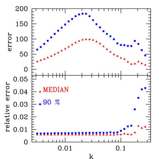
To test the accuracy of our method, we drew a random sample of $10^{3}$ of the models from our final grid that were not ruled out at more than $5\sigma$ and recomputed them from scratch with CMBfast. The results are shown in Figure 13. We see that the median accuracy of our $P(k)$-method is better than $1\%$ for $k\mathrel{\hbox to0.0pt{\lower 3.0pt\hbox{$\mathchar 536\relax$}\hss}\raise 2.0pt\hbox{$\mathchar 316\relax$}}0.15$ and never gets worse than about $1.4\%$ over our range of interest. We also tested $10^{3}$ random models from the full parameter space (without the $5\sigma$ cut on unphysical models), obtaining median errors similar to the 90% curve in Figure 13.

The only reason that equation (C3) is not exact is that neutrinos affect the growth rate of fluctuations at late times when $\Omega_{\rm k}$ and $\Omega_{\Lambda}$ become important. $f_{\nu}$ therefore cannot be separated completely from $G$. On the other hand, $f_{\nu}$ cannot be absorbed into $G$ either, since it suppresses only small-scale fluctuations. Fortunately, Figure 13 shows that equation (C3) is nonetheless very accurate in practice, breaking down badly only on scales smaller than are relevant to our present analysis. This is because at the low redshifts where $\Omega_{\rm k}$ and $\Omega_{\Lambda}$ become important, the neutrino free-streaming scale below which fluctuations are suppressed is below a few $h^{-1}{\rm Mpc}$ if $m_{\nu}>1{\rm eV}$.

Even for $f_{\nu}=0$ when equation (C3) is strictly speaking exact, the practical implementation can cause small inaccuracies. We found our $0.6\%$ “noise floor” seen in Figure 13 to be due to the horizontal shifting of the transfer function given by $h$, which we accomplished with a cubic spline. This effect is also responsible for part of the rise in relative errors towards small scales, where high baryon models have pronounced wiggles. It should be possible to eliminate this problem by computing the input transfer function grid with more finely spaced $k$-values, able to oversample all baryonic wiggles.

REFERENCES

- [1] A. E. Lange et al., astro-ph/0005004 (2000).
- [2] M. Tegmark and M. Zaldarriaga, Phys. Rev. Lett. 85, 2240 (2000).
- [3] A. Balbi et al., astro-ph/0005124 (2000).
- [4] W. Hu, M. Fukugita, M. Zaldarriaga, and M. Tegmark, astro-ph/0006436 (2000).
- [5] A. Jaffe et al., astro-ph/0007333 (2000).
- [6] W. Kinney, A. Melchiorri, and A. Riotto, astro-ph/0007375 (2000).
- [7] L. A. Kofman, N. Y. Gnedin, and N. A. Bahcall, ApJ 413, 1 (1993).
- [8] M. White, Pedro. P. T Viana P, A. R. Liddle, and D. Scott, MNRAS 283, 107 (1996).
- [9] A. R. Liddle, D. H. Lyth, T. P. T Viana, and M. White, MNRAS 282, 281L (1996).
- [10] E. F. Bunn and M. White, ApJ 480, 6 (1997).
- [11] E. Gawiser and J. Silk, Science 280, 1405 (1998).
- [12] M. Webster et al., ApJL 509, L65 (1998).
- [13] J. R. Bond and A. H. Jaffe, astro-ph/9809043 (1998).
- [14] N. Bahcall, J. P. Ostriker, S. Perlmutter,, and P. J. Steinhardt, Science 284, 1481 (1999).
- [15] B. Novosyadlyj, R. Durrer, S. Gottlb̈er, V. N. Lukash, and S. Apunevych, A&A 356, 418 (2000).
- [16] R. Durrer and B. Novosyadlyj, astro-ph/0009057 (2000).
- [17] S. L. Bridle, V. L. Eke, O. Lahav, A. N. Lasenby, M. P. Hobson, S. Cole, C. S. Frenk, and J. P. Henry, MNRAS;310;565 (1999).
- [18] S. L. Bridle et al., astro-ph/0006170 (2000).
- [19] W. Saunders et al., astro-ph/0001117 (2000).
- [20] A. J. S Hamilton, M. Tegmark, and N. Padmanabhan, astro-ph/0004334 (2000).
- [21] S. A. Shectman, S. D. Landy, A. Oemler, D. L. Tucker, H. Lin, R. P. Kirshner, P. L. Schechter, ApJ 470, 172 (1996).
- [22] E. E. Falco et al., PASP 111, 438 (1999).
- [23] A. J. S Hamilton and M. Tegmark, MNRAS 312, 285 (2000).
- [24] P. Coles, MNRAS 262, 1065 (1993).
- [25] J. N. Fry and E. Gaztañaga, ApJ 413, 447 (1993).
- [26] R. J. Scherrer and D. H. Weinberg, ApJ 504, 607 (1998).
- [27] P. Coles, A. Melott, and D. Munshi, ApJ 521, 5 (1999).
- [28] A. V. Kravtsov and A. A. Klypin, ApJ 520, 437 (1999).
- [29] P. Colín., A. A. Klypin, A. V. Kravtsov, and A. M. Khokhlov, ApJ 523, 32 (1999).
- [30] V. K. Narayanan, A. Berlind, and D. H. Weinberg, ApJ 528, 1 (2000).
- [31] A. J. Benson, S. Cole, C. S. Frenk, C. M. Baugh, and C. G. Lacey, MNRAS 314, 517 (2000).
- [32] M. Tegmark and M. Zaldarriaga, astro-ph/0002091 (2000).
- [33] G. Feldman and R. D. Cousins, Phys. Rev. D 57, 3873 (1998).
- [34] S. Burles and D. Tytler, astro-ph/9803071 (1998).
- [35] S. Burles, K. M. Nollett, J. N. Truran, and M. S. Turner, Phys. Rev. Lett. 82, 4176 (1999).
- [36] W. Freedman et al. 2000, ApJ, submitted B. K. Gibson 2000, private communication
- [37] K. Scholberg et al., hep-ex/9905016 (1999).
- [38] R. A. C Croft, W. Hu, and R. Davé, Phys. Rev. Lett. 83, 1092 (1999).
- [39] W. Hu, Nature 404, 939 (2000).
- [40] M. White, D. Scott, and E. Pierpaoli, astro-ph/0004385 (2000).
- [41] P. J. E Peebles, Principles of Physical Cosmology (Princeton, Princeton University Press, 1993).
- [42] L. M. Griffiths, D. Barbosa, and A. R. Liddle, MNRAS 308, 854 (1999).
- [43] A. Venkatesan, ApJ 537, 55 (2000).
- [44] C. H. Lineweaver, Science 284, 1503 (2000).
- [45] A. Sarajedini, B. Chaboyer, and P. Demarque, PASP 109, 1321 (1997).
- [46] A. Rosenberg, I. Saviane, G. Piotto, and A. Aparicio, Astron. J. 118, 2306 (1999).
- [47] A. J. S Hamilton M. Tegmark, astro-ph/0008392 (2000).
- [48] A. Jenkins et al. 1998 (The Virgo consortium), ApJ 499, 20 (1998).
- [49] J. A. Peacock, MNRAS 284, 885 (1997).
- [50] I. Szapudi, E. Branchini, Frenk C S et al., astro-ph/0007243 (2000).
- [51] C. Beisbart M. Kerscher, astro-ph/0003358 (2000).
- [52] E. Hawkins, S. Maddox, E. Branchini, and W. Saunders 2000, MNRAS, submitted
- [53] J. R. Bond, A. H. Jaffe, and L. E. Knox, ApJ 533, 19 (2000).
- [54] A. Melchiorri, M. V. Sazhin, V. V. Shulga, N. Vittorio, ApJ 518, 562 (1999a).
- [55] M. Tegmark, ApJL 514, L69 (1999).
- [56] J. Lesgourgues and M. Peloso, Phys. Rev. D 62, 81301 (2000).
- [57] S. Hannestad, astro-ph/0005018 (2000).
- [58] S. H. Hansen and F. L. Villante, Phys. Lett. B 486, 1 (2000).
- [59] M. Orito, T. Kajino, G. J. Mathews, and R. N. Boyd, astro-ph/0005446 (2000).
- [60] S. Esposito, G. Mangano, G. Miele, and O. Pisanti, astro-ph/0005571 (2000).
- [61] S. Esposito, G. Miele, S. Pastor, M. Peloso, and O. Pisanti, astro-ph/0005573 (2000).
- [62] S. Esposito, G. Mangano, A. Melchiorri, G. Miele, and O. Pisanti, astro-ph/0007419 (2000).
- [63] M. Kaplinghat and M. S. Turner, astro-ph/0007454 (2000).
- [64] E. Jenkins et al., ApJ 520, 182 (1999).
- [65] Sonneborn et al., astro-ph/0007238 (2000).
- [66] D. Tytler 2000, private communication
- [67] M. Fukugita, C. J. Hogan, and P. J. E Peebles, ApJ 503, 518 (1998).
- [68] M. Rauch et al., ApJ 489, 7 (1997).
- [69] D. Weinberg et al., ApJ 490, 564 (1997).
- [70] Y. Zhang et al., ApJ 495, 63 (1998).
- [71] T. Theuns et al., MNRAS 303, L58 (1999).
- [72] J. J. Mohr, Z. Haiman, and G. P. Holder, astro-ph/0004244 (2000).
- [73] R. Durrer and B. Novosyadlyj, astro-ph/0009057 (2000).
- [74] S. Perlmutter et al., Nature 391, 51 (1998).
- [75] A. G. Riess et al., Astron. J. 116, 1009 (1998).
- [76] M. White, ApJ 506, 495 (1998).
- [77] N. A. Bahcall and X. Fan, ApJ 504, 1 (1998).
- [78] V. R. Eke, S. Cole, C. S. Frenk, and J. P. Henry, MNRAS;298;1145 (1998).
- [79] J. P. Henry, ApJ 534, 565 (2000).
- [80] I. Zehavi and A. Dekel, Nature 401, 252 (1999).
- [81] A. R. Liddle and P. T. P Viana, MNRAS 303, 535 (1999).
- [82] P. J. E Peebles, The Large-Scale Structure of the Universe (Princeton, Princeton University Press, 1980).
- [83] O. Lahav, P. B. Lilje, J. R. Primack, M. J. Rees, MNRAS 251, 136 (1991).
- [84] A. J. S Hamilton, astro-ph/0006089 (2000).
- [85] A. N. Taylor, W. E. Ballinger, A. F. Heavens, and H. Tadros, astro-ph/0007048 (2000).
- [86] U. Pen, ApJ 504, 601 (1998).
- [87] A. Dekel and O. Lahav, ApJ 520, 24 (1999).
- [88] M. Tegmark and P. J. E Peebles, ApJL 500, 79 (1998).
- [89] E. Gawiser and J. Silk, astro-ph/0002044 (2000).
- [90] D. J. Eisenstein and W. Hu, ApJ 511, 5 (1999).
- [91] B. Novosyadlyj, R. Durrer, and V. N. Lukash, A&A 347, 799 (1999).
- [92] U. Seljak and M. Zaldarriaga, ApJ 469, 437 (1996). M. Zaldarriaga and U. Seljak, astro-ph/9911219 (1999).